Full Terms & Conditions of access and use can be found at
http://www.tandfonline.com/action/journalInformation?journalCode=ubes20
Download by: [Universitas Maritim Raja Ali Haji] Date: 11 January 2016, At: 22:42
Journal of Business & Economic Statistics
ISSN: 0735-0015 (Print) 1537-2707 (Online) Journal homepage: http://www.tandfonline.com/loi/ubes20
Semiparametric Estimation of Additive Quantile
Regression Models by Two-Fold Penalty
Heng Lian
To cite this article: Heng Lian (2012) Semiparametric Estimation of Additive Quantile Regression Models by Two-Fold Penalty, Journal of Business & Economic Statistics, 30:3, 337-350, DOI: 10.1080/07350015.2012.693851
To link to this article: http://dx.doi.org/10.1080/07350015.2012.693851
Published online: 20 Jul 2012.
Submit your article to this journal
Article views: 683
View related articles
Semiparametric Estimation of Additive Quantile
Regression Models by Two-Fold Penalty
Heng L
IANDivision of Mathematical Sciences, School of Physical and Mathematical Sciences, Nanyang Technological University, Singapore 637371, Singapore ([email protected])
In this article, we propose a model selection and semiparametric estimation method for additive models in the context of quantile regression problems. In particular, we are interested in finding nonzero components as well as linear components in the conditional quantile function. Our approach is based on spline approximation for the components aided by two Smoothly Clipped Absolute Deviation (SCAD) penalty terms. The advantage of our approach is that one can automatically choose between general additive models, partially linear additive models, and linear models in a single estimation step. The most important contribution is that this is achieved without the need for specifying which covariates enter the linear part, solving one serious practical issue for models with partially linear additive structure. Simulation studies as well as a real dataset are used to illustrate our method.
KEY WORDS: Oracle property; Partially linear additive models; SCAD penalty; Schwartz-type infor-mation criterion.
1. INTRODUCTION
Additive models have received considerable attention since their introduction by Hastie and Tibshirani (1990). They are more parsimonious than fully nonparametric models (Chaudhuri 1991) that are difficult to fit when the number of predictors is medium to large, and more flexible than linear models by not constraining the relationships to be linear. At a given quantile τ ∈(0,1), the additive model for quantile regression has the following form
Yi =µτ+ p
j=1
mτ,j(Xij)+ǫτ,i, i=1, . . . , n, (1)
where (Yi, Xi) are independent and identically distributed with
the same distribution as (Y, X), X=(X1, . . . , Xp)T is thep
-dimensional predictor andǫτ,iis the random error that satisfies
P(ǫτ,i≤0|Xi)=τ. Note that no distribution forǫτ,i needs to
be specified and heterogeneous errors are not excluded since ǫτ,ican depend on the covariates. The value of quantile
regres-sion has been demonstrated by a rapidly expanding literature in econometrics, social sciences, and biomedical studies [see the original article by Koenker and Bassett Jr (1978) or re-fer to Koenker (2005) for a comprehensive introduction]. As a useful supplement to mean regression, it produces a more com-plete description of the conditional response distribution and is more robust to heavy-tailed random errors. Quantile regression for additive models has previously been treated in De Gooijer and Zerom (2003), Horowitz and Lee (2005), and quantile re-gression with varying coefficients represents a class of closely related models (Kim2007; Wang, Zhu, and Zhou2009).
The additive form in the conditional quantile above circum-vents the curse of dimensionality problem in nonparametric quantile regression. However, some covariates do not have effects on the responses and we desire to find those covariates either for efficiency reasons or to make the model more easily interpretable. Such zero components in additive models can be found by performing tests or by optimizing a penalized
likelihood. To further reduce the worry of overfitting, one can try to find those parametric (i.e., linear) components. Such components typically converge faster than a truly nonpara-metric component and the resulting model, a semiparanonpara-metric additive model (or partially linear additive model), is more parsimonious than general additive models. Such advantages of a semiparametric additive model are emphasized in Opsomer and Ruppert (1999). However, it is generally difficult to determine which covariates should enter as nonparametric components and which should enter as linear components. The commonly adopted strategy in practice is just to consider continuous covariates entering as nonparametric components and discrete covariates entering as parametric. For example, in studying the impact of various possible determinants on the intention of East Germans to migrate to West Germany 1 year after the Germany unification (H¨ardle, Mammen, and M¨uller1998), some covariates may affect the response variable linearly, for instance, discrete covariates, while other covariates enter nonlinearly. This generalization allows richer and more flexible model structures than linear models and general addi-tive models. This is a reasonable approach but there is always the healthy skepticism for its efficiency if some continuous covariates have linear effects. It would be nice to have a statistical tool that can perform model selection (finding both zero and linear components) and estimation simultaneously.
Both zero components and linear components could be found by performing some hypothesis testing. However, this might be cumbersome to perform in practice whether there are more than just a few predictors to test. Given the success of the penalization approach for selecting a sparse model in Huang, Horowitz, and Wei (2010), it is highly desirable that the same approach could be applied to select parametric components as well as zero compo-nents. To the best of our knowledge, the present article is the first
© 2012American Statistical Association Journal of Business & Economic Statistics
July 2012, Vol. 30, No. 3 DOI:10.1080/07350015.2012.693851
337
to consider a penalization approach for variable selection and parametric component selection in additive quantile regression. Huang, Horowitz, and Wei (2010) considered variable selection for mean regression in additive models when p≫n. Due to technical difficulties in dealing with quantiles, we restrict our study to the fixed p case and leave the high-dimensional set-ting for the future. However, we note that several recent works (Belloni and Chernozhukov2011; Kato2011) have considered variable selection for linear quantile regression in high dimen-sions. We use a two-fold Smoothly Clipped Absolute Deviation (SCAD) penalty, originally introduced in Fan and Li (2001), one for finding zero components and the other for finding paramet-ric components. The technical difficulty lies in dealing with the penalty for finding parametric components. In terms of compu-tation, the difficulty lies in that the problem cannot be reduced to linear programming, which is the major approach to solving quantile regression problems in the literature. We note that when using only one penalty for finding zero components, our inves-tigation is reduced to that of sparse additive models in quantile regression, which is of interest in itself since quantile regression and mean regression are sufficiently different.
In the next section, we will propose the two-fold SCAD penalization procedure, and present its theoretical properties. In particular, we show that the procedure can select the true model with probability approaching one, the usual one-dimensional nonparametric convergence rate is achieved on the component functions and furthermore the slope parameters for the linear parametric components actually converge faster at the root-n
rate and are asymptotically normal. These results together show that our estimator has the oracle property. We also propose to use a Schwartz-type information criterion (SIC; also adapted to our context that includes two penalty terms) to choose the regularization parameters. In Section3, some simulations are carried out to assess the performance of the proposed method, and we also apply the method to a real dataset as illustrations. The technical proofs for the main theoretical results are provided in the Appendix.
2. TWO-FOLD SCAD PENALIZATION
2.1 Spline-Based Estimation
For the ease of presentation, we will omitτ in the expressions wherever clear from the context. Without loss of generality, we assume the distribution ofXj,1≤j ≤pis supported on [0,1],
and also impose the conditionEmj(Xj)=0 which is required
for identifiability.
At the start of the analysis, we do not know which com-ponent functions in (1) are linear or actually zero. We use polynomial splines to approximate the components. Let t0= 0< t1<· · ·< tK′ < tK′+1=1 partition [0,1] into subinter-vals [tk, tk+1), k=0, . . . , K′ withK′ internal knots. We only restrict our attention to uniform (equally spaced) knots, al-though quasi-uniform or data-driven choices can be considered. A polynomial spline of order q is a function whose restric-tion to each subinterval is a polynomial of degreeq−1 and globallyq−2 times continuously differentiable on [0,1]. The collection of splines with a fixed sequence of knots has a nor-malized B-spline basis{B1(x), . . . , BK˜(x)}with ˜K=K′+q.
Because of the centering constraint Emj(Xj)=0, we
in-stead focus on the subspace of spline functionsS0
j := {s:s=
space isK=K˜ −1 dimensional due to the empirical version of the constraint). Using spline expansions, we can approximate the components bymj(x)≈gj(x)=Kk=1bj kBj k(x). Note that it
is possible to specify a differentKfor each component but we assume that they are the same for simplicity.
Our main goal is to find both zero components (i.e.,mj ≡0)
and linear components (i.e.,mj is a linear function). The former
can be achieved by shrinkinggj to zero. For the latter, we
want to shrink the second derivativeg′′jto zero instead. This suggests the following minimization problem
( ˆµ,b)ˆ =arg min
called the check function), pλ1 and pλ2 are two penalties
used to find zero and linear coefficients, respectively, with two regularization parametersλ1andλ2, andgj =bTjBj with
bj =(bj1, . . . , bj k)T,Bj =(Bj1, . . . , Bj K)T. When the penalty
function is chosen appropriately (Tibshirani1996; Wang and Xia 2009), in the resulting estimates, somegjwill be exactly zero
and somegj′′will be exactly zero. The former obviously corre-sponds to the zero components, while the latter will correspond to the linear components, since a function has a second deriva-tive identically zero if and only if it is a linear function. The estimated component functions are ˆmj =bˆTjBj. Note that since
second derivative is commonly used in smoothing spline es-timation (Wahba1990) as well as functional linear regression (Ramsay and Silverman2005). However the purpose there is to encourage smoothness of the estimated nonparametric function and no model selection as we aim for here can be achieved. Accordingly, in the smoothing spline literature, thesquareof g′′
jis used as the penalty, which is quite different from using
the SCAD penalty as done here. For convenience, we define
Zi =(B11(Xi1), B12(Xi1), . . . , B1K(Xi1), . . . BpK(Xip))T,
Z=(Z1, . . . , Zn)T.
The minimization problem above can be written as
( ˆµ,b)ˆ =arg min
There is more than one way to specify the penalty function and here we only focus on the SCAD penalty function (Fan and Li 2001), defined by its first derivative
p′λ(x)=λ I(x≤λ)+(aλ−x)+
(a−1)λ I(x > λ)
,
witha >2 andpλ(0)=0. We will usea =3.7 as suggested
in Fan and Li (2001). The SCAD penalty is motivated by three desirable properties of a penalty function: unbiased for large signals, resulting in sparse estimates due to singularity at zero, and producing estimators continuous in data. Other choices of penalty, such as the adaptive lasso (Zou2006) or the minimax concave penalty (Zhang2010), are expected to produce similar results in both theory and practice.
2.2 MM Algorithm
Quantile regression problems are usually solved by refor-mulating them into linear programming problems and efficient solvers for linear programming are then applied. However, due to the use of penalties, reduction to linear programming is no longer possible. Instead, we use the majorization-minimization (MM) algorithm to solve (3), which is a general technique for solving complicated optimization problems [see Hunter and Lange (2004) for a nice review]. We present the method here briefly with more details on the idea found in the article by Hunter and Lange (2000).
First, the loss functionρτ(u) is approximated by its
perturba-tion for some smallǫ >0, appropriately chosen constantc. Without the penalty, at iteration k+1, the MM algorithm works by minimizing the majorizer
1
k is the residual at iterationk. The minimizer is the
new estimateµk+1, bk+1.
With the two-fold penalty, the implementation is only slightly more complicated. Similar to the loss function, the two penalties can be approximated by
Note that this is similar to the majorizer for the loss function whenτ =0.5, and is just the same as local quadratic approxi-mation advocated in Fan and Li (2001).
After these approximations, the minimization problem in each iteration is a quadratic function and can be solved in closed form. In our implementation, we set ǫ=10−8. Besides, if
Note that Hunter and Li (2005) had already shown that the above quadratic approximation for the penalty function actually majorizes a function that converges to the penalty function as ǫ→0. Thus the iterative algorithm is an MM algorithm with solution converging to the minimizer of a functional (denoted by, say, Qǫ) that closely approximates Qdefined in
Equation (3). Thus by the general property of the MM algorithm, our algorithm has a descent property, in the sense that in each iteration, it decreases the value ofQǫ. Based on
proposition 3.2 in Hunter and Li (2005) and proposition 5 in Hunter and Lange (2000),Qǫ is close toQwhen ǫ≈0. The
reader can refer to these two articles for more details. Finally, we note that ifmˆ′′
j =0, then ˆmj is a linear
func-tion and implicitly we actually get an estimate ˆβj for the slope
parameter.
The MM algorithm is very easy to implement since the so-lution has a closed-form expression at each iteration. For linear quantile regression, Wu and Liu (2009) proposed to use the difference convex algorithm (DCA) to solve the optimization problem with the SCAD penalty and showed that it is much faster than the MM algorithm. While it is certainly interesting to consider ways to speed up the numerical calculations in a similar fashion, we note that DCA cannot be directly applied in our case due to the appearance ofgjandg′′j, which makes
linear programming inapplicable even after writing the penalty as the difference of two convex functions.
2.3 Tuning Parameter Selection
In practice, to achieve good numerical performance, we need to choose several parameters appropriately. We fix the spline order to be q=4, that is, we use cubic splines in all our nu-merical examples. For the number of basis functionsK, we first fit the additive model without any penalization and use 10-fold cross-validation to selectK.
WithK determined, we propose to use an SIC to select the regularization parametersλ1andλ2simultaneously. In our con-text, a natural SIC is defined by
SICλ=log used as the smoothing parameters, d1 is the number of com-ponents estimated as nonparametric, andd2 is the number of components estimated as parametric. We will demonstrate that SIC performs well in our numerical examples.
2.4 Asymptotic Results
For convenience, we assume thatmj is truly nonparametric
for 1≤j ≤p1, is linear forp1+1≤j ≤s=p1+p2, and is zero for s+1≤j ≤p. The true components are denoted by m0j,1≤j ≤pand the true slope parameters for the parametric
components are denoted by β0=(β0,p1+1, . . . , β0s)T. Let Fi
be the cumulative distribution function and fi be the density
function of ǫi conditional on Xi1, . . . , Xis (with the
corre-sponding random element denoted byf, which depends onX). Denotef=diag{f1(0), . . . , fn(0)}.
Let X(1)=(X1, . . . , Xp1) T
and X(2)=(Xp1+1, . . . , Xs)T.
Let A denote the subspace of functions on Rp1 that take an
additive form
A:=
h
x(1)
:h(x(1))=h1(x1)+ · · · +hp1(xp1),
Ehj(Xj)2<∞andEhj(Xj)=0,
and for any random variableW withE(W2)<∞, letEA(W) denote the projection ofW ontoAin the sense that
E{f(0)(W−EA(W))(W−EA(W))}
=inf
h∈AE
f(0)
W −h
X(1)
W−h(X(1)
.
The definition ofEA(W) trivially extends to the case whereW is a random vector by componentwise projection.
Let h(X(1))
=EA(X(2)). Each component of h(X(1))= (h(1)(X(1)), . . . , h(p2)(X
(1)))T can be written in the form
h(s)(x)= p1
j=1h(s)j(xj) for some h(s)j ∈Sj0. Denote
1=Ef(0){(X(2)−h(X(1)))(X(2)−h(X(1)))T},2=Eτ(1−τ)
{(X(2)
−h(X(1)))(X(2)
−h(X(1)))T
}. These definitions are similar to those in Wang, Zhu, and Zhou (2009) for varying-coefficient models. In the case of quadratic loss, when there is only one nonparametric component (i.e., the true model is a partially linear model), we can simply define the projection E(X(2)|X1), and working with X(2)−E(X(2)|X1) to “profile out” the nonparametric part is the basic strategy used for par-tially linear models in investigating the asymptotic properties of the linear part. Our definitions above can thus be regarded as an extension for dealing with additive partially linear quantile regression models.
The following standard regularity assumptions are used.
(A1) The covariate vector X has a continuous density sup-ported on [0,1]p. Furthermore, the marginal densities for
Xj,1≤j ≤pare all bounded from below and above by
two fixed positive constants, respectively.
(A2) Fi(0)=τ, andfi is bounded away from zero and has a
continuous and uniformly bounded derivative.
(A3) Emj(Xj)=0,1≤j ≤s. mj(x) is linear inxfor p1+ 1≤j ≤s, andmj ≡0 forj > s.
(A4) For g=mj,1≤j ≤p1 or g=h(s)j,1≤s≤p2,1≤ j ≤p1,gsatisfies a Lipschitz condition of orderd >1/2:
|g(⌊d⌋)(t)
−g(⌊d⌋)(s)
| ≤C|s−t|d−⌊d⌋, where ⌊d⌋ is the
biggest integer strictly smaller than d and g(⌊d⌋) is the
⌊d⌋th derivative ofg. The order of the B-spline used sat-isfiesq ≥d+2.
(A5) The matrices1and2are both positive definite.
Theorem 1. Assume (A1)–(A5), and that K∼n1/(2d+1), λ1, λ2→0, we have the rate of convergence
m0j−mˆj2=O
n−2d2d+1,1≤j ≤p,
where ˆmj =bˆTjBj is the estimated component function.
Remark 1. Although not explicit in the convergence rate, it would be clear from the proof in the Appendix that the conver-gence rate can be written asK/n+K−2dfor a range of values of
K. The first term represents the stochastic error (asKincreases, the dimension increases), while the second term corresponds to the approximation error (asKincreases, the spline functions are more flexible). Thus there is a bias–variance trade-off in the choice ofK. We will show in the next section thatKchosen by 10-fold cross-validation works well in practice.
The next theorem shows that whenλ1, λ2 are appropriately specified, we can select the true partially linear additive model with high probability.
Theorem 2. In addition to the assumptions in Theorem 1, we assumend/(2d+1)min
{λ1, λ2} → ∞. Then with probability approaching 1,
(a) ˆmj ≡0, s+1≤j ≤p,
(b) ˆmj is a linear function forp1+1≤j ≤s.
Next, we show that for the linear components, the estimator for the slope parameter is asymptotically normal (this estimator
ˆ
βj is implicitly defined by ˆmj when ˆmj represents a linear
function). We note that the asymptotic variance is the same as when the true model is known beforehand, thus our estimator has the so-called oracle property.
Theorem 3. (Asymptotic Normality) Under the same set of assumptions as in Theorem 2, we have√n( ˆβ−β0)→ N(0, −112−11) in distribution.
Remark 2. With regard to the consistency and asymptotic normality results presented above, we should also mention the recent work by P¨otscher and coauthors (Leeb and P¨otscher 2006,2008; P¨otscher and Schneider 2009), who have studied the (uniform) consistency of estimates of distribution functions of the penalized estimators including the SCAD estimator. In particular, they have shown that if an estimator is consistent in model selection, it is impossible to possess the oracle prop-erty (asymptotic normality) uniformly in a neighborhood of zero coefficients. These results are of great interest, but uniform convergence is more relevant when many of the true regres-sion parameters are very close to zero, which commonly arises in cases where the number of parameters (in our context, the number of parameters in the linear part) diverges with sample size. Although we acknowledge that taking the parameters in our model to be fixed is partly subjective and in some cases modeling the parameters as changing with sample size is more appropriate, the oracle property for fixed parameter is still an important issue.
Finally, in the same spirit of that of Wang, Li, and Tsai (2007), we come to the question of whether the SIC can identify the true model in our setting.
Theorem 4. Under assumptions (A1)–(A5) and that K∼ n1/(2d+1), as assumed in Theorem 1, the parameters ˆλ
1, ˆλ2 se-lected by SIC can select the true model with probability ap-proaching 1.
3. NUMERICAL EXAMPLES
3.1 Simulation Studies
We conducted Monte Carlo studies for the following iid and heteroscedastic error model
Yi = p
j=1
mj(Xij)+(1+ |Xi1|)
ei−Fe−1(τ)
, (4)
withm1(x)=3 sin(2π x)/(2−sin(2π x)),m2(x)=6x(1−x), m3(x)=2x,m4(x)=x,m5(x)= −x,p=10 so that five com-ponents are actually zero, andFe(.) denotes the distribution
func-tion of the mean zero errorei. Thus in our generating model, the
number of nonparametric components isp1=2 and the number of nonzero linear components isp2=3. Several simulation sce-narios are considered. For sample size, we setn=100 or 200, forτ we considerτ =0.25 and 0.5, foreiwe consider a normal
distribution with standard deviation 0.2,and a Student’s t dis-tribution with scale parameter 0.2 and degrees of freedom 2. To generate the covariates, we first letXij be marginally standard
normal with correlations given by cov(Xij1, Xij2)=(1/2)| j1−j2|,
and then apply the cumulative distribution function of the stan-dard normal distribution to transformXij to be marginally
uni-form on [0,1]. When generating data from (4) withτ =0.5, we use the quadratic loss function (mean regression) as well as ρ0.5to perform estimation for comparison. For any loss function used, we compute four estimators, including the oracle estima-tor where the nonparametric and the parametric components are correctly specified with no penalty used, our estimator with the two-fold SCAD penalty, the sparse additive estimator where only the first SCAD penalty is used (thus it performs variable selection but does not try to find the parametric components), and finally the linear quantile regression model with a SCAD penalty. We use 10-fold cross-validation to selectKand use SIC to select the regularization parameters in both our estimator and the sparse additive estimator with a single penalty. The imple-mentations are carried out on an HP workstation xw8600 in R software.
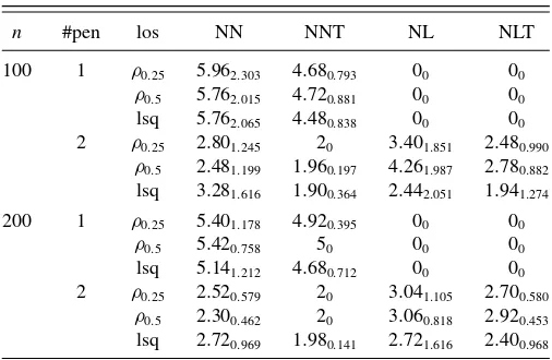
For all scenarios, 100 datasets are generated and the results are summarized in Tables1–7. In Table 1, we investigate the model selection results for both our estimator and the sparse additive estimator with one single penalty, when the errors are Gaussian. For both estimators, we see SIC successfully selected the nonzero components, with increased sample size resulting in slightly better performance. Our estimator can further dis-tinguish between nonparametric and parametric components. Furthermore, when data are generated from (4) withτ =0.5, the results from quantile regression (median regression) and least squares regression are similar.Table 2reports the model selection results for errors with t distribution.
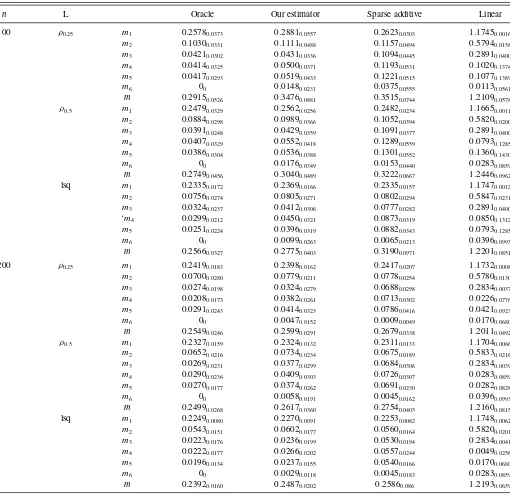
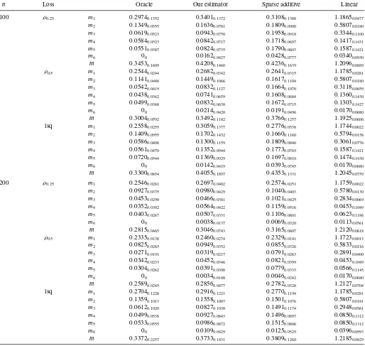
Tables3 and4, for Gaussian random errors and Student’st
errors, respectively, contain root mean squared errors (RMSE) for the first six component functions (note the sixth component is actually zero), which is defined by
RMSEj =
1
T
T
i=1
( ˆmj(ti)−mj(ti))2,
Table 1. Model selection results for our estimator and the sparse additive estimator, both using SIC for model selection, when errors
are Gaussian
n #pen loss NN NNT NL NLT
100 1 ρ0.25 6.102.012 4.980.141 00 00
ρ0.5 5.821.480 4.960.197 00 00
lsq 5.461.034 50 00 00
2 ρ0.25 2.661.061 20 4.061.973 2.700.788
ρ0.5 2.721.278 20 3.461.643 2.720.814
lsq 2.821.137 20 2.861.578 2.541.002
200 1 ρ0.25 5.160.509 50 00 00
ρ0.5 5.260.527 50 00 00
lsq 5.100.303 50 00 00
2 ρ0.25 2.340.658 20 3.281.143 2.900.614
ρ0.5 2.320.652 20 3.161.149 2.900.646
lsq 2.260.564 20 3.000.857 2.940.564
NOTE: NN: average number of nonparametric components selected; NNT: average number of nonparametric components selected that are truly nonparametric (or truly nonzero for sparse additive estimator with one penalty); NL: average number of linear components selected; NLT: average number of linear components selected that are truly linear. The numbers in smaller fonts are the corresponding standard errors; #pen being 1 indicates the sparse additive estimator with one single penalty and #pen being 2 indicates our estimator with two-fold penalty;ρ0.25andρ0.5denote the quantile regressions (with check function as the loss function) and “lsq” denotes the least squares regression (mean regression).
on a fine grid (t1, . . . , tT) consisting of 500 points equally spaced
on [0,1]. We also show the RMSE for the regression function m=10
j=1mj. For data generated from (4) withτ =0.5, we
also compare the performance of median regression with least squares regression. On the nonparametric components (m1and m2), the errors for estimators with a single penalty (sparse ad-ditive model) and double penalties are similar, and both are qualitatively close to those of the oracle estimator. However, for the parametric components, our estimator with the two-fold penalty is obviously more efficient, leading to about 40%∼50% reduction in RMSE. The estimation results for the 0.25 quantile are slightly worse than those for the 0.5 quantile. As expected, least squares regression is better than median regression in es-timation when the errors are Gaussian, and worse than median regression when the errors aret2. We also performed simula-tions for the Cauchy random errors (Student’stwith degree of freedom 1), and in this case, the advantage of median regression
Table 2. Model selection results when random errors are distributed ast2
n #pen los NN NNT NL NLT
100 1 ρ0.25 5.962.303 4.680.793 00 00
ρ0.5 5.762.015 4.720.881 00 00
lsq 5.762.065 4.480.838 00 00
2 ρ0.25 2.801.245 20 3.401.851 2.480.990
ρ0.5 2.481.199 1.960.197 4.261.987 2.780.882
lsq 3.281.616 1.900.364 2.442.051 1.941.274
200 1 ρ0.25 5.401.178 4.920.395 00 00
ρ0.5 5.420.758 50 00 00
lsq 5.141.212 4.680.712 00 00
2 ρ0.25 2.520.579 20 3.041.105 2.700.580
ρ0.5 2.300.462 20 3.060.818 2.920.453
lsq 2.720.969 1.980.141 2.721.616 2.400.968
Table 3. Root mean squared errors form1, . . . , m6, mfor the four different estimators, when errors are Gaussian
n L Oracle Our estimator Sparse additive Linear
100 ρ0.25 m1 0.25780.0373 0.28810.0557 0.26230.0303 1.17450.0016
m2 0.10300.0331 0.11110.0488 0.11570.0494 0.57940.0158
m3 0.04210.0302 0.04310.0336 0.10940.0445 0.28910.0400
m4 0.04140.0325 0.05000.0371 0.11930.0531 0.10200.1374
m5 0.04170.0293 0.05190.0433 0.12210.0515 0.10770.1389
m6 00 0.01480.0231 0.03750.0555 0.01130.0561
m 0.29150.0526 0.34760.0881 0.35150.0744 1.21090.0578
ρ0.5 m1 0.24790.0329 0.25620.0256 0.24820.0234 1.16650.0011
m2 0.08840.0298 0.09890.0366 0.10520.0394 0.58200.0200
m3 0.03910.0248 0.04290.0359 0.10910.0377 0.28910.0400
m4 0.04070.0329 0.05520.0418 0.12890.0559 0.07930.1285
m5 0.03860.0304 0.05360.0388 0.13010.0552 0.13600.1430
m6 00 0.01760.0349 0.01530.0440 0.02830.0859
m 0.27490.0456 0.30400.0489 0.32220.0667 1.24460.0962
lsq m1 0.23350.0172 0.23690.0166 0.23350.0157 1.17470.0012
m2 0.07560.0274 0.08050.0271 0.08020.0294 0.58470.0231
m3 0.03240.0237 0.04120.0306 0.07770.0282 0.28910.0400
‘m4 0.02990.0212 0.04500.0321 0.08730.0319 0.08500.1312
m5 0.02510.0224 0.03960.0319 0.08820.0343 0.07930.1285
m6 00 0.00990.0263 0.00650.0213 0.03960.0993
m 0.25660.0327 0.27750.0403 0.31900.0971 1.22010.0851
200 ρ0.25 m1 0.24190.0183 0.23980.0162 0.24170.0207 1.17320.0008
m2 0.07000.0280 0.07790.0211 0.07780.0254 0.57800.0130
m3 0.02740.0198 0.03240.0279 0.06880.0298 0.28340.0037
m4 0.02080.0173 0.03820.0261 0.07130.0302 0.02260.0776
m5 0.02910.0243 0.04140.0323 0.07860.0416 0.04210.0923
m6 00 0.00470.0152 0.00090.0049 0.01700.0680
m 0.25490.0246 0.25990.0291 0.26790.0338 1.20110.0492
ρ0.5 m1 0.23270.0159 0.23240.0132 0.23110.0133 1.17040.0066
m2 0.06520.0216 0.07340.0234 0.06750.0189 0.58330.0216
m3 0.02690.0231 0.03770.0299 0.06840.0306 0.28340.0039
m4 0.02900.0236 0.04090.0303 0.07260.0307 0.02830.0859
m5 0.02700.0177 0.03740.0262 0.06910.0230 0.02820.0828
m6 00 0.00580.0191 0.00450.0162 0.03960.0993
m 0.24990.0268 0.26170.0360 0.27540.0403 1.21600.0815
lsq m1 0.22490.0080 0.22700.0091 0.22530.0082 1.17480.0062
m2 0.05430.0151 0.06020.0177 0.05600.0164 0.58200.0201
m3 0.02230.0176 0.02360.0199 0.05300.0194 0.28340.0041
m4 0.02220.0177 0.02660.0202 0.05570.0244 0.00490.0256
m5 0.01960.0134 0.02370.0155 0.05400.0166 0.01700.0680
m6 00 0.00290.0118 0.00450.0183 0.02830.0859
m 0.23920.0160 0.24870.0202 0.25860.086 1.21930.0659
NOTE: The numbers in smaller fonts are the corresponding standard errors.
is much more obvious (not reported here). The linear estima-tors obviously do not perform well for data simulated from a semiparametric model.
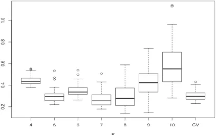
Now we use the case n=100, τ =0.5 with normally distributed errors to study the sensitivity of the estimation results to the tuning parameters, and demonstrate that both 10-fold cross-validation (for choosingK) and SIC (for choosing λ1 andλ2) work well empirically.Figure 1shows the RMSE for K=4,5, . . . ,10 as well as for K selected by 10-fold cross-validation. Hereλ1andλ2are chosen by SIC in all cases. It is seen that the RMSE does not change much forKranging from 5 to 8. For larger K, the effect of overfitting begins to appear. The 10-fold cross-validation works very well in this simulation. Table 5 shows that in terms of model selection, K=4 andK=5 are the best with 10-fold cross-validation still
achieving a good accuracy. Next we useK chosen by 10-fold cross-validation and consider the sensitivity of the results to λ1andλ2. Let (ˆλ1,λˆ2) be the tuning parameters found by SIC, and in Figure 2, we compare the RMSE when using tuning parameters (cλˆ1, cλˆ2), for c∈ {0.1,0.25,0.5,0.75,1,1.5,2} (note thatc=1 just produces the original results when tuning parameters are selected by SIC). We see that SIC also has a reasonably good performance. Usingc≥1.5 results in much larger RMSE. There is little overfitting whencis small, which is not surprising since when p is small compared with the sample size as in our simulations, overfitting is not expected to be severe even if no penalization is used. On the other hand, as Table 6shows, tuning parameters selected by SIC produce rea-sonable model selection accuracy, while usingctoo small is not advisable.
Table 4. Root mean squared errors when errors aret2
n Loss Oracle Our estimator Sparse additive Linear
100 ρ0.25 m1 0.29740.1352 0.34010.1372 0.31080.1388 1.18650.0477
m2 0.13490.0555 0.16360.0781 0.18090.0900 0.58070.0180
m3 0.06190.0523 0.09430.0750 0.19580.0918 0.33440.1100
m4 0.05840.0523 0.08420.0717 0.17180.0697 0.14170.1431
m5 0.05510.0387 0.08240.0735 0.17900.0603 0.15870.1421
m6 00 0.01620.0427 0.04280.0777 0.03400.0930
m 0.34530.1609 0.42080.1460 0.42360.1639 1.20960.0889
ρ0.5 m1 0.25440.0244 0.26820.0342 0.26410.0315 1.17850.0281
m2 0.11410.0488 0.14490.1066 0.16170.1104 0.58070.0180
m3 0.05420.0419 0.08320.1127 0.16640.1070 0.31180.0859
m4 0.04380.0362 0.07410.0659 0.16080.0684 0.13600.1430
m5 0.04990.0368 0.08320.0638 0.16720.0715 0.13030.1427
m6 00 0.02140.0420 0.01910.0496 0.01700.0680
m 0.30040.0592 0.34920.1182 0.37660.1257 1.19250.0606
lsq m1 0.25580.0255 0.30590.1377 0.27760.0538 1.17440.0022
m2 0.14090.0955 0.17020.1432 0.16600.1160 0.57940.0158
m3 0.05860.0408 0.13000.1159 0.18090.0840 0.30610.0776
m4 0.05610.0470 0.13520.0944 0.17730.0769 0.15870.1421
m5 0.07200.0544 0.13690.0929 0.16970.0810 0.14740.1430
m6 00 0.01420.0419 0.03930.0745 0.01700.0680
m 0.33000.0854 0.40550.1897 0.43530.1331 1.20450.0759
200 ρ0.25 m1 0.25460.0281 0.26970.0402 0.25740.0251 1.17590.0022
m2 0.09270.0375 0.09800.0429 0.10400.0403 0.57800.0130
m3 0.04530.0290 0.04660.0381 0.10210.0425 0.28340.0069
m4 0.03520.0302 0.05640.0422 0.11590.0516 0.04530.1049
m5 0.04030.0267 0.05070.0331 0.11060.0601 0.06230.1186
m6 00 0.00380.0137 0.00690.0320 0.01130.0561
m 0.28150.0465 0.30460.0743 0.31650.0607 1.21200.0618
ρ0.5 m1 0.23350.0138 0.24600.0274 0.23290.0141 1.17230.0013
m2 0.08250.0265 0.09490.0352 0.08550.0326 0.58330.0216
m3 0.02710.0191 0.03190.0217 0.07910.0263 0.28910.0400
m4 0.03420.0233 0.04520.0346 0.08210.0399 0.04530.1049
m5 0.03040.0262 0.03910.0308 0.07790.0333 0.05660.1145
m6 00 0.00340.0148 0.00460.0242 0.01700.0680
m 0.25890.0245 0.28560.0477 0.27820.0328 1.21270.0704
lsq m1 0.27040.1228 0.29160.1221 0.27700.1194 1.17850.0281
m2 0.13590.1013 0.15580.1087 0.15010.1076 0.58070.0181
m3 0.06120.1020 0.08270.1038 0.14910.1174 0.29480.0561
m4 0.04990.0538 0.09270.0843 0.14960.0897 0.08500.1312
m5 0.05330.0555 0.09860.0872 0.15150.0806 0.08500.1312
m6 00 0.01090.0429 0.01250.0529 0.03960.0993
m 0.33720.2257 0.37330.1431 0.38090.1260 1.21850.0829
Table 5. Model selection results whenKchanges from 4 to 10, compared with the results whenKis chosen by 10-fold
cross-validation (CV)
K NN NNT NL NLT
4 2.861.143 20 3.481.403 2.520.706
5 2.661.205 20 3.781.887 2.460.930
6 3.681.910 20 2.861.784 1.901.015
7 3.882.066 20 2.462.042 1.761.187
8 5.063.046 20 2.062.333 1.341.394
9 8.902.296 20 0.281.050 0.140.571
10 9.860.989 20 0.060.424 0.060.424
CV 2.721.278 20 3.461.643 2.520.814
Table 6. Model selection results when using (cλˆ1, cλˆ2) as the
regularization parameters in the penalties, where (ˆλ1,λˆ2) are the
parameters found from SIC
c NN NNT NL NLT
0.1 9.221.233 20 0.500.735 0.200.451
0.25 7.401.564 20 1.881.271 0.920.922
0.5 4.481.631 20 3.441.774 1.840.997
0.75 3.001.087 20 4.021.911 2.460.838
1 2.721.278 20 3.461.643 2.520.814
1.5 2.280.671 20 3.761.623 2.820.522
2 2.100.462 20 3.681.463 2.860.495
Table 7. Prediction errors for the three estimators on independently simulated data. RMSE and AD are the root mean squared prediction errors and the absolute deviation prediction errors, respectively, as defined in the main text
Oracle Our estimator Sparse additive
Error n Loss RMSE AD RMSE AD RMSE AD
Normal 100 ρ0.5 0.357 0.140 0.389 0.157 0.445 0.178
lsq 0.337 0.134 0.358 0.145 0.383 0.153 200 ρ0.5 0.317 0.122 0.327 0.129 0.342 0.134
lsq 0.300 0.118 0.309 0.123 0.321 0.127
Student’st 100 ρ0.5 0.383 0.155 0.460 0.188 0.540 0.217
lsq 0.410 0.166 0.544 0.219 0.583 0.235 200 ρ0.5 0.318 0.123 0.339 0.134 0.355 0.139
lsq 0.382 0.153 0.450 0.180 0.484 0.194
Finally inTable 7, we compare the prediction errors for three estimators, when data are generated from (4) withτ =0.5. Both median regression and least squares regression are considered. We use two prediction accuracy measures including RMSE and absolute deviation, which are defined by
1
n′ n′
i=1
(Yi−Yˆi)2
and
1 n′
n′
i=1
|Yi−Yˆi|,
respectively, where Yi, i=1, . . . , n′=200 are the responses
of an independently simulated testing dataset and ˆYi are the
fitted values for the different methods. Comparing our estima-tor with the sparse additive estimaestima-tor, our estimaestima-tor has better performance, which is probably due to the more efficient
es-timates for the parametric part. Comparing median regression with least squares regression, the relative performances depend on the error distribution as before.
3.2 Real Data
Now we illustrate the methodology with real data used by Yafeh and Yosha (2003) to investigate the relationship between shareholder concentration and several indices for managerial moral hazard in the form of expenditure with scope for private benefit. The dataset includes a variety of variables describing more than 100 Japanese industrial chemical firms listed on the Tokyo stock exchange. (The dataset is available online through the Economic Journal at http://www.res.org.uk.) This dataset was also used in Horowitz and Lee (2005) as an application of additive models for median regression which is more flexible than the linear model used in Yafeh and Yosha (2003). We use the general sales and administrative expenses deflated by sales
Figure 1. RMSE changes whenKchanges from 4 to 10, andKchosen by 10-fold cross-validation (CV) works well in terms of RMSE. This simulation is based onn=100,τ=0.5 with normal errors.
Figure 2. RMSE changes whenλ1andλ2change. The label on thex-axis is the multiplicative factor on bothλ1andλ2chosen by SIC. For
example, the left-most boxplot is obtained by using a smallλ1andλ2obtained by multiplying the tuning parameters found by SIC by a factor of
0.1, while the boxplot labeled by “1” is the results using tuning parameters obtained from SIC.
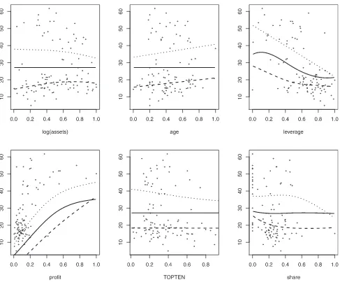
Figure 3. The fitted response values for the Moral Hazard data when one covariate varies and others fixed at 0.5, at quantile levelsτ=0.25 (dashed),τ=0.5 (solid), andτ =0.75 (dotted).
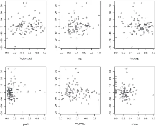
Figure 4. Scatterplots for the estimated residuals versus the covariates forτ=0.5. The assumption that the errors have median zero is visually reasonable for the estimated errors.
(denoted by MH5) as the response variableY which is one of five measures of activities with a scope for managerial moral hazard in Yafeh and Yosha (2003). We use more covariates, a total of six, than those used in Horowitz and Lee (2005) though, including log(assets), the age of the firm, leverage (ratio of debt to total assets), profit (variance of operating profitability of firms between 1977 and 1986), TOPTEN (the percentage of ownership held by the 10 largest shareholders), and share (share of the largest creditor in total debt). All covariates are normalized by a linear transformation to lie in [0,1] before analysis. The sample size turns out to be 114 after removing firms with some covariates missing.
InFigure 3, we show the fitted values of the responses as one covariate varies while others are fixed at 0.5, at quantile levels 0.25,0.5,and 0.75. At these three levels, we identified 5,3,and 6 nonzero components, and 2,0,and 3 linear (nonzero) com-ponents, respectively. The marginal relationship between each covariate and MH5 may differ depending on the quantile of in-terest. It is interesting to note that although some covariates are not related to responses for median regression, they have some effects at lower and/or upper quantiles. In particular, the
covari-ate TOPTEN, which is the main covaricovari-ate of interest in the study of moral hazard, is only estimated to have nonzero effect at the upper quantile. In other words, firms with a more concentrated ownership structure spend less on activities with a scope for managerial moral hazard, but this effect seems to be only re-stricted to the upper tail of the expenses distribution. Variability of firm performance has an increasing effect on MH5, which was nevertheless not found in Yafeh and Yosha (2003). Inspection of the data scatterplots inFigure 3reveals that these features cap-tured in the estimates are driven by the data and are not simply an artifact of the model. In contrast to Horowitz and Lee (2005) who found that log(asset), age, leverage, and TOPTEN are all sig-nificantly nonlinear based on confidence intervals without bias correction, three of these (except leverage) are estimated as zero in median regression in our method. Note that leverage is indeed the most significant predictor as in Horowitz and Lee (2005). We also fitted the unpenalized additive model and found that the resulting estimates were similar to those reported in Horowitz and Lee (2005) and thus the differences are mainly attributed to the use of penalties. Although Horowitz and Lee (2005) claimed that all four predictors are significant based on pointwise 90%
confidence intervals, while we find three of these (except lever-age) are zeros, we note that based on their confidence intervals, indeed a major portion of the confidence intervals for these three component functions overlaps zero and deviations from zero mainly appear at the very beginning or the very end of the estimated component functions. The penalization approach is obviously different from the testing approach. In particular, the penalization approach explicitly gives a selected model by trad-ing off model fitttrad-ing with model parsimony, while when one uses testing, one needs to combine the marginal testing results some-how to get a final model. Furthermore, we also think that for testing the significance of the component functions, simultane-ous confidence bands would be more appropriate than pointwise confidence intervals, if possible to obtain, which will be wider than the pointwise confidence intervals. And thus one would conjecture that those three predictors might not be significant based on simultaneous confidence bands.
Although it is not clear what caused these differences, the scatterplots show that our estimates are at least reasonable. We also think penalized estimates are more stable. The residual plots shown inFigure 4suggest also the fitting is good. The results are very similar whenλ1andλ2are multiplied by a scalar factor in the range from 0.7 to 1.3, andKin the range from 5 to 7.
Finally, we note that inFigure 3, there is some crossing of the quantile curves for covariate values close to 0 and 1. Such cross-ing problems are well known in the quantile regression literature, and could be addressed by the algorithm proposed in, say, Cher-nozhukov, Fern´andez-Val, and Galichon (2010). This however requires that the quantile estimators be obtained on a fine grid of quantile levels. We do not pursue this idea further in this work.
4. CONCLUSION
In this article, we show that it is possible to select both zero components and linear components, as well as perform estima-tion, in a single step for additive quantile regression models. The difficulty of correctly specifying a partially linear additive model seems to be the main obstacle for the wide application of the semiparametric model, despite its many advantages. Thus, we believe that our work has made some progress in arguing for its usefulness and applicability.
Although we demonstrated that using SIC to selectλ1andλ2 resulted in consistent model selection, we do not have similar theoretical results for selectingKbased on cross-validation. We note that theories for cross-validation were mainly developed for linear models as well as in the context of kernel sion and density estimation. In the context of quantile regres-sion, or additive models, or nonparametric estimation based on B-splines, we cannot find similar results for cross-validation in the literature. Thus, we mainly rely on our simulation studies to demonstrate that the data-driven choice works well in practice. Alternatively, as suggested by a referee, one can selectKbased on cross-validation with least squares loss, for which theoretical guarantees are available (Li1987; Li and Racine2007). Whether this would work well in our model, especially for relatively large or small values ofτ, remains to be seen.
After the first version of the article was submitted, we learned that model selection using two penalties to simultaneously de-termine the zero and linear components was studied in Zhang, Cheng, and Liu (2011), for mean regression (with quadratic
loss function). Besides the difference that they used smoothing splines to approximate the nonparametric components, they did not use a penalty shrinking the second derivative of the com-ponent function. Instead their method is based on an explicit decomposition of a general nonlinear function into a linear part and a nonlinear part and then shrinking the nonlinear part to zero. Furthermore, they did not satisfactorily demonstrate the model selection consistency of their approach due to the difficulty in dealing with smoothing splines (they only proved consistency for the special case where the nonparametric components are periodic functions and conjectured that it is generally true). In terms of computation, using smoothing splines, the number of basis coefficients is proportional to the sample size, while for polynomial splines, the number of basis coefficients is propor-tional toK, which is typically chosen to be less than 10 in the literature. We will report our detailed study on mean regression based on polynomial splines in another article (Lian, Chen, and Yang2011).
APPENDIX
In the proofs,Cdenotes a generic constant that might assume different values at different places. Let b0=(b01T, . . . , b
be the parametric vector that includes the intercept (appropriately normalized), and similarly a:= (√Kµ, bT)T. Let Z˜
We note that, based on well-known properties of B-spline, Dj has eigenvalues of order 1/K,Ej is of rankK−1, and all
its positive eigenvalues are of order 1/K.
The main idea of our proofs is summarized as follows. To show the asymptotic results, we first show that since the tuning parametersλ1andλ2are sufficiently small, the convergence rate is basically same as the estimator without penalty. On the other hand, since we assumeλ1 andλ2 cannot converge to zero too fast, if the correct model is not selected, we can construct an estimator that achieves a smaller value on the objective function which will lead to a contradiction. Finally, since we show that the correct model is selected with high probability, the asymptotic normality of the linear components follows from that of the oracle estimator.
×
independent ofXibut the arguments go through without change
under our heterogeneous setup.]
Again by the Cauchy–Schwartz inequality, the first term in (A.3) is bounded by
The above convergence rate can be further improved toaˆ− a02=Op(K2/n+1/K2d−1) as follows. First note that since
with probability tending to 1. Removing the regularizing terms in (A.1) and following the same reasoning as before, the rates are improved toaˆ−a02 =Op(K2/n+1/K2d−1).
The rates of convergence forbˆj−b0j2immediately imply
Proof of Theorem 2. We only show part (b) as an illustration and part (a) is similar. Suppose for some p1 < j ≤s, ˆbTjBj
does not represent a linear function. Define ˆb∗to be the same as
ˆ
bexcept that ˆbj is replaced by its projection onto the subspace
{bj :bTjBj represents a linear function}. Similarly as before, we
As in the proof of Theorem 1, we have
Ppλ1
and thus with probability approaching 1 (since ˆb∗T
j Ejbˆ∗j =0),
On the other hand, since
by the definition of the SCAD penalty function. What is left is only to showaˆ−aˆ∗ = bˆj −bˆj∗ =Op(
zero eigenvalue. Thus by the characterization of eigenvalues in terms of Rayleigh quotient, ( ˆbj−bˆ∗j)
TE
j( ˆbj −bˆj∗)/bˆj −bˆ∗j 2
lies between the minimum and the maximum positive eigenval-ues ofEj, which is of order 1/K.
Proof of Theorem 3. We note that because of Theorem 2, we only need to consider a correctly specified partially linear additive model without regularization terms. This is very similar to partially linear varying-coefficient models studied in Wang, Zhu, and Zhou (2009) and the arguments used there can be followed line by line here, showing the asymptotic normality of the slope parameter. The reason is that in their arguments, for example, they only used the properties of covariate matrices, such as that eigenvalues of ˜ZTZ˜ are of orderOp(n/K), which
are also true here for additive models.
Proof of Theorem 4. For any regularization parametersλ= (λ1, λ2), we denote the corresponding minimizer of (3) by ˆaλ=
(√Kµˆλ,bˆλ) and denote by ˆa=(
√
Kµ,ˆ b) the minimizer whenˆ the optimal sequence of regularization parameters is chosen such that ˆb represents the correct model with optimal convergence rates. There are four separate cases to consider.
Case 1, bˆT
λjBj represents a linear component for some
j ≤p1.Similar to the calculations performed in the proof of Theorems 1 and 2 [see Equations (A.2), (A.3) and the argu-ments following (A.4)], we have
1
Since the true mj is not linear and ˆbj is consistent in model
selection, aˆ−aˆλ2/K is bounded away from zero and thus
Z˜( ˆa−aˆλ)2/nis at least of orderOp(1) (i.e., bounded away
from zero). Note that this lower bound is uniform for allλin Case 1. Thus [noting n1
for any 0≤C1, C2≤p, with probability tending to 1 and the SIC cannot select suchλ.
Case 2, bˆλj is zero for some1≤j ≤s.The above case, as
well as Case 1, results in underfitted models and the proof is very similar and therefore omitted.
Case 3, bˆT
λjBj represents a nonlinear component for some
p1 < j ≤s.Here when considering Case 3, we implicitly ex-clude all previous cases, that is, no underfitting occurs. We define ˆa∗ as the unregularized estimator that minimizes (3)
without the two penalty terms, but constrained to represent the same model as ˆaλ. By definition, we immediately have
iρ(Yi−Z˜iaˆλ)≥iρ(Yi−Z˜iaˆ∗) and then (by the same
ar-guments concerningGiand ˜Gi above)
1
with probability tending to 1 (also uniformly for all suchλ).
Case 4, bˆλj is nonzero for somej ≥s. The above case is
similar to Case 3 and thus the proof is omitted.
ACKNOWLEDGMENTS
The author thanks Professor Hirano, an associate editor, and two referees for their careful reading and constructive comments that greatly improved the manuscript.
[Received March 2011. Revised March 2012.]
REFERENCES
Belloni, A., and Chernozhukov, V. (2011), “L1-Penalized Quantile Regression in High-Dimensional Sparse Models,”The Annals of Statistics, 39(1), 82– 130. [338]
Chaudhuri, P. (1991), “Nonparametric Estimates of Regression Quantiles and Their Local Bahadur Representation,”The Annals of Statistics, 19(2), 760– 777. [337]
Chernozhukov, V., Fern´andez-Val, I., and Galichon, A. (2010), “Quantile and Probability Curves Without Crossing,”Econometrica, 78(3), 1093–1125. [347]
De Boor, C. (2001),A Practical Guide to Splines(rev. ed.), New York: Springer-Verlag. [349]
De Gooijer, J. G., and Zerom, D. (2003), “On Additive Conditional Quantiles With High-Dimensional Covariates,”Journal of the American Statistical Association, 98(461), 135–146. [337]
Fan, J. Q., and Li, R. Z. (2001), “Variable Selection via Nonconcave Penalized Likelihood and Its Oracle Properties,”Journal of the American Statistical Association, 96(456), 1348–1360. [338,339,339]
H¨ardle, W., Mammen, E., and M¨uller, M. (1998), “Testing Parametric Versus Semiparametric Modeling in Generalized Linear Models,”Journal of the American Statistical Association, 93(444), 1461–1474. [337]
Hastie, T., Tibshirani, R. (1990), “Monographs on Statistics and Applied Proba-bility,”Generalized Additive Models(1st ed.), London: Chapman and Hall. [337]
He, X., and Shi, P. (1994), “Convergence Rate of B-Spline Estimators of Nonparametric Conditional Quantile Functions,”Journal of Nonparametric Statistics, 3(3), 299–308. [348]
——— (1996), “Bivariate Tensor-Product B-Splines in a Partly Linear Model,” Journal of Multivariate Analysis, 58(2), 162–181. [348]
Horowitz, J. L., and Lee, S. (2005), “Nonparametric Estimation of an Additive Quantile Regression Model,”Journal of the American Statistical Associa-tion, 100(472), 1238–1249. [337,344,346]
Huang, J., Horowitz, J. L., and Wei, F. (2010), “Variable Selection in Non-parametric Additive Models,”The Annals of Statistics, 38(4), 2282–2313. [337]
Hunter, D., and Li, R. (2005), “Variable Selection Using MM Algorithms,”The Annals of Statistics, 33(4), 1617–1642. [339]
Hunter, D. R., and Lange, K. (2000), “Quantile Regression via an MM Al-gorithm,”Journal of Computational and Graphical Statistics, 9(1), 60–77. [339]
——— (2004), “A Tutorial on MM Algorithms,”The American Statistician, 58(1), 30–37. [339]
Kato, K. (2011), “Group Lasso for High Dimensional Sparse Quantile Regres-sion Models,” Arxiv preprint arXiv:1103.1458. [338]
Kim, M. (2007), “Quantile Regression With Varying Coefficients,”The Annals of Statistics, 35, 92–108. [337]
Koenker, R. (2005), “Econometric Society Monographs,” inQuantile Regres-sion, Cambridge: Cambridge University Press. [337]
Koenker, R., and Bassett Jr, G. (1978), “Regression Quantiles,”Econometrica: Journal of the Econometric Society, 46(1), 33–50. [337]
Leeb, H., and P¨otscher, B. (2006), “Performance Limits for Estimators of the Risk or Distribution of Shrinkage-Type Estimators, and Some General Lower Risk-Bound Results,”Econometric Theory, 22(01), 69–97. [340] ——— (2008), “Sparse Estimators and the Oracle Property, or the Return of
Hodges’ Estimator,”Journal of Econometrics, 142(1), 201–211. [340] Li, K. (1987), “Asymptotic Optimality forCp,Cl, Cross-Validation and
Gener-alized Cross-Validation: Discrete Index Set,”The Annals of Statistics, 15(3), 958–975. [347]
Li, Q., and Racine, J. (2007),Nonparametric Econometrics: Theory and Prac-tice, Princeton NJ: Princeton University Press. [347]
Lian, H., and Chen, X., and Yang, J. (2011), “Identification of Partially Lin-ear Structure in Additive Models With an Application to Gene Expression Prediction From Sequences,” Biometrics. Available athttp://onlinelibrary. wiley.com/doi/10.1111/j.1541-0420.2011.01672.x/abstract[347]
Opsomer, J. D., and Ruppert, D. (1999), “A Root-n Consistent Backfitting Es-timator for Semiparametric Additive Modeling,”Journal of Computational and Graphical Statistics, 8(4), 715–732. [337]
P¨otscher, B., and Schneider, U. (2009), “On the Distribution of the Adaptive LASSO Estimator,”Journal of Statistical Planning and Inference, 139(8), 2775–2790. [340]
Ramsay, J. O., and Silverman, B. W. (2005),Functional Data Analysis(2nd ed., Springer Series in Statistics), New York: Springer. [338]
Tibshirani, R. (1996), “Regression Shrinkage and Selection via the Lasso,” Journal of the Royal Statistical Society,Series B, 58(1), 267–288. [338] Wahba, G. (1990),Spline Models for Observational Data, Philadelphia PA:
Society for Industrial and Applied Mathematics. [338]
Wang, H., Li, R., and Tsai, C. L. (2007), “Tuning Parameter Selectors for the Smoothly Clipped Absolute Deviation Method,”Biometrika, 94(3), 553– 568. [340]
Wang, H. J., Zhu, Z., and Zhou, J. (2009), “Quantile Regression in Partially Linear Varying Coefficient Models,”The Annals of Statistics, 37(6B), 3841– 3866. [337,340,349]
Wang, H. S., and Xia, Y. C. (2009), “Shrinkage Estimation of the Varying Co-efficient Model,”Journal of the American Statistical Association, 104(486), 747–757. [338]
Wei, Y., and He, X. (2006), “Conditional Growth Charts,”The Annals of Statis-tics, 34(5), 2069–2097. [348]
Wu, Y., and Liu, Y. (2009), “Variable Selection in Quantile Regression,” Statis-tica Sinica, 19(2), 801–817. [339]
Yafeh, Y., and Yosha, O. (2003), “Large Shareholders and Banks: Who Monitors and How?,”The Economic Journal, 113(484), 128–146. [344,346] Zhang, C. (2010), “Nearly Unbiased Variable Selection Under Minimax
Con-cave Penalty,”The Annals of Statistics, 38(2), 894–942. [339]
Zhang, H. H., Cheng, G., and Liu, Y. (2011), “Linear of Nonlinear? Automatic Structure Discovery for Partially Linear Models,”Journal of the American Statistical Association, 106(495), 1099–1112. [347]
Zou, H. (2006), “The Adaptive Lasso and Its Oracle Properties,”Journal of the American Statistical Association, 101(476), 1418–1429. [339]