Full Terms & Conditions of access and use can be found at
http://www.tandfonline.com/action/journalInformation?journalCode=ubes20
Download by: [Universitas Maritim Raja Ali Haji] Date: 13 January 2016, At: 00:47
Journal of Business & Economic Statistics
ISSN: 0735-0015 (Print) 1537-2707 (Online) Journal homepage: http://www.tandfonline.com/loi/ubes20
Efficient Estimation of Conditional Asset-Pricing
Models
Douglas J Hodgson & Keith P Vorkink
To cite this article: Douglas J Hodgson & Keith P Vorkink (2003) Efficient Estimation of
Conditional Asset-Pricing Models, Journal of Business & Economic Statistics, 21:2, 269-283, DOI: 10.1198/073500103288618954
To link to this article: http://dx.doi.org/10.1198/073500103288618954
View supplementary material
Published online: 24 Jan 2012.
Submit your article to this journal
Article views: 56
Ef’cient Estimation of Conditional
Asset-Pricing Models
Douglas J.
Hodgson
Département des Sciences Économiques, Université du Québec, Montréal, Québec, Canada H3C 3P8 (hodgson.douglas-james@uqam.ca)
Keith P.
Vorkink
Marriott School of Management, Brigham Young University, Provo, UT 84602 (kpv3@email.byu.edu)
A semiparametric efcient estimation procedure is developed for the parameters of multivariate gen-eralized autoregressive conditional heteroscedasticity-in-mean models when the disturbances have a conditional distribution assumed to be elliptically symmetric but otherwise unrestricted. Under high-level assumptions, the resulting estimator achieves the asymptotic semiparametric efciency bound. The elliptical symmetry assumption allows us to avert the curse of dimensionality problem that would oth-erwise arise in estimating the unknown error distribution. This framework is suitable for the estimation and testing of conditional asset-pricing models, such as the conditional capital asset-pricing model. We apply our procedure in an empirical study of stock prices, with Monte Carlo simulation results also reported.
KEY WORDS: Capital asset-pricing model; Multivariate autoregressive conditional heteroscedastic-ity; Semiparametric efciency.
1. INTRODUCTION
Modeling expected returns has permeated much of nancial research over the past three decades. The payoffs from a cor-rect relationship between risk and expected return are abun-dant and include applications to capital budgeting, portfolio performance, event studies, and others. The conditional mean-variance model of the risk–return relationship was initially implemented empirically for multivariate time series data by Bollerslev, Engle, and Wooldridge (1988), who developed a conditional capital asset-pricing model (C-CAPM) and associ-ated generalized autoregressive conditional heteroscedasticity-in-mean (GARCH-M) econometric model. A large empirical literature has subsequently developed in this area, gener-ally estimating the models with Gaussian quasi-maximum likelihood estimation (Q-MLE) techniques. Although such techniques typically retain their consistency and asymptotic normality properties in the presence of nonnormal data (Bollerslev and Wooldridge 1992), asymptotic inefciency and imprecise parameter estimates can occur due to the presence of thick tails in the distributions of nancial data. We propose a new estimation methodology for the multivariate GARCH-in-mean model designed to account for excess tail thickness by adopting a exible distributional assumption of conditional elliptical symmetry. The estimator will achieve the asymptotic semiparametric efciency bound in the presence of general elliptical symmetry in the data-generating process. We apply our estimator to a dataset of stock returns and perform asset-pricing tests of the C-CAPM.
It has been well documented that stock returns are not inde-pendent and identically distributed (iid) normal. In particular, they tend to exhibit substantial kurtosis and have moments that vary over time (see, e.g., Mandelbrot 1963; Fama 1965; Engle 1982; Bollerslev, Chou, and Kroner 1992). These phenomena are not unrelated. It is well known that time-varying volatil-ity implies a thick-tailed unconditional distribution. However, as shown by Bollerslev (1987), conditional volatility cannot
completely account for the tail behavior of the unconditional distribution in nancial returns (see also Diebold 1988; Nelson 1991; Vorkink 2001). Accurate description of return distribu-tions should include modeling of both of these properties.
We propose a semiparametric efcient estimator that attempts to improve on the inefciencies that may occur in the Gaussian Q-MLE when thick tails are present in the dis-tribution of the standardized innovations to the GARCH-M model. To do so, we assume the distribution of returns to be a member of the class of elliptically symmetric distribu-tions. This class includes those having conditional dependence among higher moments, innite variance (Cauchy), Studentt, and others. (For further discussion of elliptical distributions, see Fang, Kotz, and Ng 1990; Muirhead 1982; the Appendix of this article.) We derive the asymptotic semiparametric ef-ciency bound for the estimation of our model’s parameters in the presence of an unknown elliptically symmetric innovation density, then propose a semiparametric estimator that achieves the bound. This estimator uses a nonparametric kernel estima-tor of the unknown innovation density.
This assumption of elliptical symmetry plays an integral role in our estimation methodology, particularly in the esti-mation of the residual density. We can think of two extreme methods of obtaining an estimate of a leptokurtokic residual density. One method is to t a fully parametric nonnormal distribution to the residuals. Alternatively, the density could be estimated in a fully nonparametric fashion. For example, Drost and Klaassen (1997) proposed a semiparametric ef-cient estimation method for univariate GARCH models that involves nonparametric kernel estimation of the innovation
©2003 American Statistical Association Journal of Business & Economic Statistics April 2003, Vol. 21, No. 2 DOI 10.1198/073500103288618954
269
density. However, their method is difcult to extend to a mul-tivariate setting, due to the “curse of dimensionality” prob-lem, in which the convergence rate of a nonparametric density estimate diminishes rapidly as the dimension of the density increases.
Elliptical symmetry provides a middle ground between a fully specied Q-MLE approach and a fully nonparametric approach. Whereas the density is nonparametrically estimated within the elliptically symmetric class, this restriction allows us to do so without falling prey to the “curse of dimensional-ity.” Specically, we are able to transform the nonparametric density estimator to one that is always one-dimensional.
This estimator’s roots lie in Bickel’s (1982) adaptive esti-mator. Assuming iid data, Bickel considered the problem of adaptively estimating mean and covariance parameters in ellip-tically symmetric location models. He found that under the assumption of elliptical symmetry, the mean could be tively estimated and the covariance parameters could be adap-tively estimated up to a scale. Linton (1993) showed that slope parameters can be adaptively estimated in a regression model with ARCH errors when the innovation density is symmetric. In both cases, the innovation density is otherwise unrestricted and is estimated using nonparametric kernel methods. Hodg-son, Linton, and Vorkink (in press) have derived adaptive esti-mators in time series models under the assumption of elliptical symmetry using a nonparametric estimate of the joint innova-tion density.
Hodgson et al. (in press) developed an estimator of lin-ear unconditional asset pricing models under elliptical sym-metry. Their estimator is fully asymptotically efcient and places no assumptions on the family of return distributions other than that this family is elliptically symmetric. They found that the more general estimator leads to substantially different estimates and conclusions when testing unconditional asset-pricing models. However, the treatment of conditional heteroscedasticity is ad hoc, which results in potential inef-ciencies. This article extends this work by parameterizing the conditional heteroscedasticity in the form of a multivari-ate GARCH-M model with conditionally elliptically symmet-ric innovation distributions.
Asset-pricing theory exists that is consistent with the speci-cation of elliptical symmetry, at least for the case of the one-period unconditional CAPM, although the conditions under which these results would extend to a multiperiod condi-tional model are not known. Merton (1973) mentioned the restrictions required in a multiperiod model to generate one-period-ahead mean-variance pricing. It may be possible to show that Merton’s (1973) conditions, along with conditional elliptical symmetry, yield such pricing, but we know of no formal results to this effect. In the one-period CAPM, the assumption of normally distributed returns is sufcient, but not necessary, for a mean-variance result. Chamberlain (1983), Owen and Rabinovitch (1983), and Berk (1997) have obtained mean-variance pricing under the assumption that returns are elliptically symmetric. In fact, Berk (1997) found that ellip-tical symmetry is the most general distributional assumption that is consistent with mean-variance maximization when con-sumers are assumed to have concave utility functions. These exact-pricing models are more general and consistent with
the empirical regularities than their normal distribution coun-terparts. However, although these theoretical results can be obtained with more general distributional assumptions, estima-tion of the general model has not been feasible until recently. Our estimator is specically designed to be more efcient than the Gaussian Q-MLE in the presence of thick tails in the standardized innovations to the GARCH-M model. As shown by Bollerslev and Wooldridge (1992), the Q-MLE has the virtue of being consistent and asymptotically normal for a sub-stantial range of deviations of the innovations from iid normal-ity. We have not been able to derive similar properties for the semiparametric estimator developed in this article, and know its properties only when the assumption of iid elliptical sym-metry on the innovations holds. For data where such deviations from this assumption as conditional or unconditional skewness may be present, we can currently only conjecture as to the behavior of our estimator. Furthermore, empirical and simula-tion evidence reported herein suggests that the efciency gains of our estimator vis-à-vis the Q-MLE are quite modest for estimation of conditional mean parameters, although the evi-dence suggests that there may be potential gains in estimating conditional covariance parameters and conditional betas.
The article is organized as follows. Section 2 introduces the conditional CAPM model that we estimate and test. Section 3 presents our multivariate GARCH-M econometric model. Section 4 contains our derivation of the semiparametric ef-ciency bound for our model and describes a method of feasibly computing an estimator that will achieve the bound. Sections 5 and 6 report empirical and simulation results, and Section 7 concludes. The Appendix contains a discussion of elliptically symmetric densities and discusses some computational details relating to our estimator.
2. CONDITIONAL RETURN MODELS
It has been shown that the assumption of constant return distributions is not necessary to obtain equilibrium pricing equations. Merton (1973) derived an intertemporal CAPM that showed how investors would react to changing invest-ment opportunity sets. In an empirical setting, Bollerslev et al. (1988) estimated C-CAPM covariances assuming that the covariance matrix of returns followed a GARCH-M41115 process. They found that under this model’s parameterization, beta and the market price of risk are time-varying. They also showed that both returns and volatility are predictable and time-varying, in fact, they are able to predict a larger portion of the variability in returns than the unconditional counterpart (see also Harvey 1991; Buse, Korkie, and Turtle 1994; Braun, Nelson, and Sunier 1995; Jagannathan and Wang 1996). We suggest that a natural extension would be to estimate a CAPM where the residual distribution is assumed to be thick-tailed relative to the normal distribution and allow some exibility in the form of the conditional distribution.
We now introduce the C-CAPM return relationship. Our discussion closely follows that of Bollerslev et al. (1988), with some variations as suggested by, for example, DeSantis and Gerard (1997). The following equation demonstrates the main relationship of the C-CAPM, stating that the excess return on
asseti is linear in its covariance with the market portfolio,
Etƒ16Ri1 t7ƒrftD‹covtƒ14Rm1 t1 Ri1 t50 (1)
We assume that there are n assets in the market,Ri1 t is the return on asseti in periodt,Rm1 t is the return on the market portfolio,rft is the return to a risk-free asset, and the sub-scripts on expectations and covariances indicate conditional moments. Note that it would be a straightforward matter to extend the model to allow for multiple factors to inuence returns. From (1), we can see that the expected return on the market portfolio is
Etƒ16Rm1 t7ƒrftD‹vartƒ14Rm1 t51
so that the parameter ‹ can be interpreted as the market price on risk. Following DeSantis and Gerard (1997), we may treat this parameter either as a constant or as time-varying. In the latter case, it can be modeled as being dependent on an `-vector of state variables vt, and (1) can be generalized by writing‹Dexp4ƒ0üCvTtÃ15. In the model with a constant price of risk, we have ‹Dexp4ƒ0ü5. We can also write our expected return relationship as
Etƒ16Ri1 t7ƒrftDEtƒ16Rm1 tƒrft7‚i1 t1
where‚i1 tDcovtƒ14Rm1 t1Ri1 t5
vartƒ14Rm1 t5 is the conditional “beta” for asseti
in periodt.
Dene the n-vectorrtDRtƒrft‰n, whereRt is the vector of returns on the individual assets andÉn is ann-vector of 1s. Following Bollerslev et al. (1988), let×tƒ1be then-vector of weights assigned to the assets in computing the “market,” so thatRm1 tD×T
tƒ1Rt. Allowing for a possibly time-varying mar-ket price of risk, we may then write our CAPM relationship at timetfor our cross-section of assets as
Etƒ1rtDexp
¡
ƒ0üCvTtÃ1
¢
èt×tƒ11 (2)
whereèt is the covariance matrix of asset returns conditional on information available up to periodtƒ1. Note that our vec-tor of conditional betas is given by
ÂtD èt×tƒ1 ×T
tƒ1èt×tƒ1
0 (3)
Estimation of our model depends on the specication of a model for our conditional covariance matrix.
Testing the C-CAPM typically involves estimating the model
rtDÁCexp¡ƒü 0Cv
T tÃ1
¢
èt×tƒ1Cut1 (4)
where an intercept is included to capture persistent variation in rtnot captured by variation in the market return. One common test of the asset-pricing model takes the form
H02 iD01 iD11 : : : 1 n1 (5)
which implies that no signicant excess returns are present in each portfolio’s return that cannot be explained by variation
in the market portfolio return. This hypothesis can be tested by construction of a standard Wald test,
JD QÁ0dvar4ÁQ5ÁQ1 (6)
where ÁQ is an estimator anddvar4ÁQ5estimates its asymptotic covariance matrix. If this statistic deviates signicantly from 0, then we conclude that the C-CAPM does not fully explain the deviations in returns.
It is also interesting to look at the time series of the implied betas, ‚i1 t, to see whether the conditional variance parame-terization leads to substantial time variation in the covariation between the asset’s return and the market return. For exam-ple, Bollerslev et al. (1988) found substantial variation in the implied betas of their estimation of the U.S. stock and bond market, whereas Braun et al. (1995), using a modeling frame-work that differs from ours in a number of respects, found little variation in conditional betas.
3. THE ECONOMETRIC MODEL
The regression model that we estimate is given in (4). To arrive at a completely specied econometric model, we must characterize our conditional covariance matrixèt and our dis-turbance process8ut9. There is no theory predicting a GARCH model of volatility; however, a relatively parsimonious model of time-varying second moments has been quite successful in capturing the time series behavior of volatility. Our general model of conditional volatility is a simplied version of the multivariate GARCH model described by Engle and Kroner (1995),
ètDexp4Š5Ht1 (7)
where
HtDCC TC
Autƒ1u T
tƒ1ACDHtƒ1D1
CD
2 6 6 6 6 4
1 0 ¢ ¢ ¢ 0
00
0 0 00 000 00
0 0 00 0 cn1 ¢ ¢ ¢ ¢ ¢ ¢ cnn
3 7 7 7 7 51
(8)
and the matrices A andD are diagonal. This model is less general than that developed by Engle and Kroner (1995), in which
HtDCTCC n
X
jD1
Ajutƒ1uTtƒ1AjC n
X
jD1
DjHtƒ1Dj0
We adopt this simplication for computational purposes. Our model still has the generality to allow for systematically time-varying conditional variances and covariances. Other empirical articles, such as those by Bollerslev et al. (1988) and DeSantis and Gerard (1997), use simplied GARCH-M models. This specication is more general than those of Bollerslev (1987) and Jeantheau (1998) in that it allows for time-varying condi-tional covariances. Note that under our assumptions onAand D, our restriction of the leading term of C to be unity does
not entail any further loss of generality. To see this, note that the conditional variance of the rst element ofut is
vartƒ14u1t5D‘111 tDexp4Š5
¡
1Ca2 1u
2 11 tƒ1Cd
2 1h111 tƒ1
¢
1
which is the usual expression for conditional variance in a univariate GARCH model.
To complete our specication of the model, we assume that our regression disturbances8ut9have the elliptically symmet-ric conditional density
ptƒ14ut5D —èt—ƒ
1 2gQ¡uT
tèƒ 1 t ut
¢
0 (9)
Our objective in this article is to obtain a semiparametric ef-cient estimator of the parameters of our model, treating the functional form ofgQ as an unknown innite-dimensional nui-sance parameter. The function g4Q ¢5 has only a scalar as its
argument, which plays an important role in the nonparametric estimation of the density. We also deneìp1 t to be the condi-tional information matrix ofptƒ14ut5; it is proportional to the inverse of Ht and èt. We have ìp1 tDconst¢èƒt1, with the constant greater than or equal to 1. (It equals 1 ifptƒ14ut5is Gaussian.) Mitchell (1989) computed the value of the constant for various elliptically symmetric densities.
Note that because we are treatinggQ as being of unknown functional form, we can also write the density as
ptƒ14ut5D —Ht—ƒ1 2g¡uT
tHƒ 1 t ut
¢
1 (10)
where the constant of proportionality relatingHt and èt has now been absorbed into the functiong. This specication fol-lows the example of Linton (1993), who did not consider efcient estimation of Š. Note that g4Q ¢5 as dened in (9) is the density function of the iid spherically symmetrically dis-tributed random variableèƒ1=2
t ut with unit covariance matrix. As dened in (10),g4¢5 is still the density of an iid spheri-cally distributed random variable, but without the restriction of a unit covariance matrix. We also do not concern ourselves with efcient estimation ofŠ, and we rewrite our regression model as
rtDÁCexp¡
ƒ0CvTtÃ1¢
Ht×tƒ1Cut1 (11)
where ƒ0 DŠCƒ0ü. We do not consider semiparameteric efcient estimation of the parameters Š and ƒü
0 separately (although in principle it would be possible to do so), but con-sider only their sum,ƒ0. We justify this parameterization in our case because our parameters of primary interest are the intercept parameterÁand the conditional beta vectorÂt. Note that the latter depends only on the parameters of the function Ht as dened in (7), because
ÂtD èt×tƒ1 ×T
tƒ1èt×tƒ1
D exp4Š5Ht×tƒ1 ×T
tƒ1exp4Š5Ht×tƒ1
D Ht×tƒ1 ×T
tƒ1Ht×tƒ1 0
Let 411cT5T Dvech4C5, so that c is the n4nC15ƒ2 2 -vector of unknown elements of C, aDdiag4A5, dDdiag4D5, and È2 D8cT1aT1dT9T is the vector of unknown parameters in the conditional covariance function. Note that there are h2D
n4nC55ƒ2
2 parameters in È2. Likewise, let the vector of param-eters in the conditional mean function be given by È1 D 8ÁT1ÃT9T, where ÃD4ƒ
01Ã T 15
T, so that È
1 is of dimension h1DnC`C1. Our h4Dh1Ch25-dimensional full parame-ter vector is Ȳ4ÈT
11È T 25
T, which is usually estimated using
Q-MLE procedures resulting from a specication of iid nor-mality for the normalized disturbance processØtD8Hƒ
1=2 t ut9. Although few analytical results are available, Bollerslev and Wooldridge (1992) have shown, under high-level assump-tions, that the Gaussian Q-MLE will be pT-consistent and asymptotically normal, even under distributional misspecica-tion. We derive estimators that are asymptotically semipara-metrically efcient under our elliptical symmetry assumption (along with high-level assumptions similar to those of Boller-slev and Wooldridge 1992), but without placing additional restrictions on the return distribution. We use a semiparametric Newton–Raphson-type estimator following the basic approach of Bickel (1982).
4. EFFICIENT ESTIMATION
In this section we give our derivation of a semiparamet-ric efciency bound for the aforementioned model. Follow-ing the literature in the area of multivariate GARCH mod-els, we derive our estimation theory under a set of high-level assumptions. The restrictions that such assumptions imply for the parameters of our model are not known and presumably could be obtained only with great difculty. This is an endemic problem in multivariate GARCH modeling. Jeantheau (1998) provided a recent example of a consistency result for a mul-tivariate GARCH model that does not rely on such high-level assumptions, but at the cost of using a very restric-tive parameterization. We assume that our data are stationary and ergodic, that conditional variances are always nite and bounded away from 0, and that the score function has nite variance. Any expectation or derivative taken in the following sections is assumed to exist, and conditions for the consistency and asymptotic normality of the estimators used are assumed to hold. We can apply a result of Brown and Hodgson (2002) to obtain a semiparametric efciency bound for our model, which necessitates that we make the further assumptions that g4w5 is three times differentiable with bounded third deriva-tive, wherewD˜T˜, that ln—H
t4È5ƒ1=2— is three times differ-entiable with respect to Èwith bounded third derivative, and thatØt4È5is three times differentiable with respect toÈ.
We now turn to the issue of semiparametric efcient esti-mation of the parameter vector È. (For a fuller discussion of semiparametric efciency bounds and the related concepts used here, see Newey 1990.) We must derive an expression for theefcient scoreforÈ, the orthogonal complement of the projection of the score forÈonto thetangent space, which is, loosely speaking, the space spanned by all scores for param-eterizations Ò of the unknown density g4¢5 that include the true model of g4¢5as special cases. Such a parameterization,
which we write as g4uT t4È5Hƒ
1
t 4È5ut4È51Ò5, is known as a
parametric submodel. A semiparametric efciency bound for our model can be obtained by applying theorem 1 of Brown and Hodgson (2002), which applies to a class of nonlinear models with elliptical distributions that contains our model. We now give an heuristic derivation of the bound.
The log-likelihood for the aforementioned parametric sub-model for a sample of size T, where we follow the usual practice of conditioning on initial observations whose uncon-ditional density is assumed to have an asymptotically negligi-ble effect on analysis of the likelihood, is
ln¬ with respect to the nuisance parameterÒ is
`t’4È1Ò5Dg24wt4È51Ò5 g4wt4È51Ò5
1
where gj4¢1¢5denotes the partial derivative ofg with respect to its jth argument, for jD112. Note that because 8wt4È59
The tangent space´ is the innite-dimensional Hilbert space spanned by all functions having the dening characteristics of `t’4È1Ò5, namely that it is a function only ofØTØand that it has zero mean,
´ D8s4ØTØ5 2 E6s4ØTØ57D090
The projection of an arbitrary function
R4rt1rtƒ11rtƒ21 : : : 3Ht4È51Htƒ14È51 : : : 3
vt1vtƒ11 : : : 3Øt1Øtƒ11 : : : 5DR4yt5
on the tangent space can be shown to be
Pr6R4yt5—´7DE6R4yt5—ØTØ70
In calculating the efcient score forÈ, we rst consider the score forÈ, which for observationt can be written as
`tˆ4È1Ò5D ƒ1 È to prevent cluttered notation. In considering the projection of`tˆ4È1Ò5onto the tangent space, rst note that the rst two components of`tˆ4È1Ò5are orthogonal to the nuisance scores `t’4È1Ò5 for any parametric submodel and hence are orthog-onal to the tangent space. Considering the rst component on the right side of (12), we have
E
¡È andHt are both measurable with respect toëtƒ1, yielding
consider the projection of the third component of the right side of (12) onto the tangent space, which is given by
E
with the equality holding because Ht is independent of Øt. Note thatE6vec4ØtØT
t5—wt76DE6vec4ØtØTt57. Here and in what follows, we drop the nuisance parameterÒ from our notation, because the notion of a parametric submodel has served its purpose and we now concern ourselves with the semiparamet-ric model. The derivative ofg4¢5is now denoted byg04
¢5.
The projection of the periodtscore for Èonto the tangent space is, therefore,
and the periodtefcient score forÈis
Our efcient score function for the sample of sizeT is then
ãT4È5D T
X
tD1
ãt1 T4È51 (14)
with the semiparametric efcient estimator ÈQüü
T being that
Under the high-level assumptions outlined at the start of this section, the semiparametric efcient estimator will have the asymptotic distribution
where the semiparametric efciency bound¢ is given by
¢D©
Note that under our assumptions, an information matrix equal-ity will hold here, so that
E£
Note that under any misspecication (such as, e.g., the fail-ure of either our iid assumption or our elliptical symmetry assumption on the errors) this equality will fail to hold, so the possibility exists of a White (1982)-style specication test. However, we do not explore this possibility here.
If we had available a pT-consistent preliminary estimator O
ÈT, the Gaussian Q-MLE for example, and if we furthermore
knew the functional form of the density g4¢5 and the
expec-tations E6¡4vecHtƒ15T we could compute the following one-step iterative estimator, which would be asymptotically equivalent to the semiparamet-ric efcient estimatorÈQüü
T :
with the asymptotic covariance matrix estimated by
"
As an alternative information estimator in (16) and in the com-putation of standard errors, we could use
"
Of course, it is infeasible to compute ÈQü
T, because the afore-mentioned density and expectation functions are unknown. We must therefore replace these quantities with nonparamet-ric estimates, for which purpose we draw on existing results of Brown and Hodgson (2002) and Hodgson et al. (in press). To estimateE6¡4vecHƒt15T
¡È is difcult to calculate, as are the derivatives ¡uTt
¡È and ¡ln—Ht—
¡È , which also appear in our expression for the score. These difculties are discussed in the Appendix. To estimate the conditional expectation func-tionE6vec4ØtØT
t5—wt7, we make use of the fact that for ellip-tically symmetric distributions, the random n-vectorØ has a distribution (conditional on wDØTØ) that is uniform on the 4nƒ15-dimensional hypersphere with radiuspw. As Brown and Hodgson (2002) observed, the desired conditional expec-tation can be estimated to an arbitrarily high degree of preci-sion by bution on a hypersphere with radiuspwtandMis chosen suf-ciently large to achieve the desired degree of precision. The Øü
i are easily computed, as pointed out by Werner Ploberger. Draw an iid sequence8ØQi9MiD1from then-dimensional standard normal, then compute
We now consider the problem of deriving nonparamet-ric estimates of the functions g4¢5 and g04
¢5. We closely
follow the discussion of Hodgson et al. (in press). Using our preliminary estimator OÈT, we compute the standardized residuals8Øt4ÈOT59T
tD1 and the sequence of scalars wt4ÈOT5D
ØT
t4ÈOT5Øt4ÈOT5for everytD11 : : : 1 T. Next, compute the trans-formationztD’4wt5, where the transformation ’ 4¢5 belongs
to the Box–Cox (1964) family,
’4wt5Dw † tƒ1
† 0
We now compute kernel estimates of the density functionƒ4z5 of the transformed random variable z, and of its derivative ƒ04z5, and use these estimates to indirectly obtain estimates of the ratio gg4w504w5. Dene the kernelK‘T4¢5, with a bandwidth
parameter‘T, and use the kernel to compute the following estimates:
t4z5to estimate the ratio gg4w504w5 as follows:
O
if trimming conditions hold, 0 otherwise
¡z —. The trimming conditions referred to in (19) will depend on the kernel used. For certain kernels, such as the quartic or the logistic, trimming will not be required. In the Appendix, we provide expressions for the trimming conditions in the case where a Gaussian kernel is used. Even in this case, very little trimming (i.e., less than 1% of the observations) has been shown, in another context (Hodgson 1998), to yield semiparametric estimators that work well in Monte Carlo sim-ulations.
Finally, we have our semiparametric estimator for the period tscore,
where the expectation and score estimators are as dened in (17), (18), and (19) and where
We then have our semiparametric score estimator for the sam-ple of sizeT,
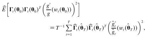
Our last step in deriving a semiparametric efcient estimator ofÈis to come up with a consistent semiparametric estimator of the expected outer product of the score. To this end, note that
To establish (21), note that
E
In place of the unknown expectation,
E
we can compute the semiparametric estimator
b
E
µ
ât4È05ât4È05T
³
g0
g4wt4È055
´2¶
DTƒ1 T
X
tD1 b
ât4OÈT5âbt4ÈOT5T
³
O g0
t O gt
4wt4ÈOT55
´2
1
where gO0t
O
gt4wt5is as dened in (19). We then have the
informa-tion estimator
b
©4OÈT5D1 4T
ƒ1 T
X
tD1
¡ln—Ht4ÈOT5— ¡È
¡ln—Ht4ÈOT5— ¡ÈT
CEb
µ
ât4È05ât4È05T
³
g0
g4wt4È055
´2¶
0
Our semiparametric efcient estimatorÈQT is then computed in the natural manner,
Q
ÈT D OÈTƒTƒ 1b©
4ÈOT5ƒ 1b
ãT4ÈOT50 (22)
The asymptotic covariance matrix of ÈQT is consistently esti-mated by©bƒ14ÈO
T5. The resulting semiparametric estimator can be shown to achieve the efciency bound using arguments of Hodgson et al. (in press) combined with those of Linton (1993) and Drost and Klaassen (1997).
As stated in Section 1, we have no analytical results on the asymptotic behavior of ÈQT when our iid elliptical symmetry assumption fails, an important consideration for data where some form of conditional or unconditional asymmetry may be present. Consequently, we can only conjecture as to this behavior. Hodgson (2000) analyzed the robustness to misspec-ication of semiparametric estimators for a much simpler class of model than is considered here, and it is not clear whether analogous arguments can be applied to the GARCH-M model. However, as a crude check on the robustness of our estimator to skewness, we have allowed for skewed innovations in our Monte Carlo experiment reported in Section 6.
5. EMPIRICAL ANALYSIS
Many econometric tests of the CAPM were published shortly after the development of the theory and have consis-tently found their way into the nance journals ever since (see, e.g., Campbell, Lo, and MacKinlay 1997 for a survey). Early empirical work seemed to support the CAPM (see Black, Jensen, and Scholes 1972; Fama and MacBeth 1973). The pri-mary methodology used in these early works was to perform cross-sectional regressions of mean returns on estimated betas (which were estimated from some preliminary time series regressions) and other putative variables and thus to test the linearity restriction of the theory. The main econometric prob-lem with this approach is the errors in variables probprob-lem that arises from the rst-stage regressions; one approach to this was to group stocks together into portfolios, thereby reducing the estimation error. By grouping according to some factor that might also affect returns, like size, one can improve the power of the test. Most modern tests of the CAPM have been
based on the multivariate regression model (see, e.g., Gibbons 1982; Stambaugh 1982).
It has also become apparent that nancial asset returns have distributions that are not constant. This has led to the test-ing of CAPMs such as the C-CAPM. The articles by Boller-slev et al. (1988) and Harvey (1989, 1991) are well-known examples where C-CAPM models are estimated and tested, and the possibility of time-varying conditional betas has also been investigated by Braun et al. (1995). Our approach here is to estimate a C-CAPM using our model discussed previously, and then test the model in the traditional framework discussed earlier. The model that we estimate is a simplied version of (11),
rtDÁCexp4ƒ05Ht×tƒ1Cut1 (23)
where we restrict the market price of risk to be constant. This could be easily relaxed by including instruments; however, to keep the analysis simple, we impose this restriction. The hypothesis tests of the C-CAPM that we use are the Wald statistics discussed in Section 2. It is standard in this literature to work with Wald statistics. Linton and Steigerwald (2000) suggested a method of computing nonparametric likelihood ratio statistics when the likelihood is unspecied, but attempts to apply this method in our model and in the unconditional model of Hodgson et al. (in press) yielded tests with very erratic behavior, so we do not report any likelihood ratio test results here.
We use our semiparametric procedure to test the C-CAPM on a dataset of daily stock returns. Our dataset consists of returns generated from the CRSP dataset of stock returns and includes daily observations from January 1996–December 1997, with a sample size of 759. For this time period, we construct three portfolios generated by sorting rms traded on the NYSE, AMEX, and NASDAQ according to size (mar-ket value). On each trading day, rms are placed into quar-tiles according to the NYSE quartile rm size breakpoints. Daily value-weighted returns are then constructed for the rms in each of the quartiles. We construct three portfolios using the quartile returns. The rst portfolio consists of a value-weighted return of the rst two quartiles. We place both of these quartiles into one portfolio primarily due to their small relative market value. After combining the two quartiles into one portfolio, we still nd daily relative weights around 1% of the market. The other two portfolios are constructed using the last two quartiles’ returns. The returns on these three port-folios and their corresponding market weights are then used to estimate and test the C-CAPM.
Table 1 provides the summary statistics for the annualized portfolio excess returns rtƒrf t, and Table 2 provides some group statistics on our three portfolio returns as well as resid-uals from the Q-MLE estimations. Multivariate normality is rejected using either the univariate kurtosis estimates or the Jarque–Bera (1980) tests performed on the individual series reported in Table 1. The multivariate measures of kurtosis also reject normality, as seen in Table 2. It appears that a substan-tial portion of the excess kurtosis is generated by time-varying second moments, as evidenced by the decline in the test statis-tic from the unconditional series to the conditionally weighted
Table 1. Summary Statistics
Portfolios Mean Std. Dev. Min Max Kurtosis J-B
Size 1 0276 10870 ƒ190377 80510 730313ü 111513ü
Size 2 0255 20231 ƒ210590 90548 460721ü 61747ü
Size 3 0332 20799 ƒ240301 150453 450721ü 21890ü
NOTE: This table provides statistical characteristics of the portfolios of excess returns used in our empirical analysis. The stock returns are obtained from the CRSP dataset. The series are daily returns from January 1995–December 1997. Estimates of kurtosis have been scaled so that under the assumption of normality the statistics have an asymptotic N(011)distribution. J-B refers to the Jarque-Bera (1980) test for normality.
üRefers to a rejection of the hypothesis that the given moment is consistent with the normal
distribution at the .01 level.
series. Although the GARCH model removes some of the lep-tokurtosis, the conditional residual distribution still contains sufcient kurtosis to lead to a rejection of normality. Box– Pierce (1970) tests (not reported) on the squared residuals indicate that autocorrelation may still be present in the second moments. We did not increase the order of our GARCH41115 model because of added estimation complexities that would ensue. However, an application of Beran’s (1979) test of ellip-tical symmetry fails to reject the hypothesis that the weighted excess returns and residuals are distributed elliptically sym-metric at the 10% level, as seen in Table 2.
Table 3 reports the results of estimating an unconditional version of (23) using ordinary least squares (OLS). The OLS estimates are consistent with the empirical literature in that the estimates of ‚ are positive and the estimates of are close to 0 relative to their standard errors. For the size 1 portfolio, the intercept is positive and statistically signicant, suggesting that excess returns are generated by holding a portfolio of small stocks.
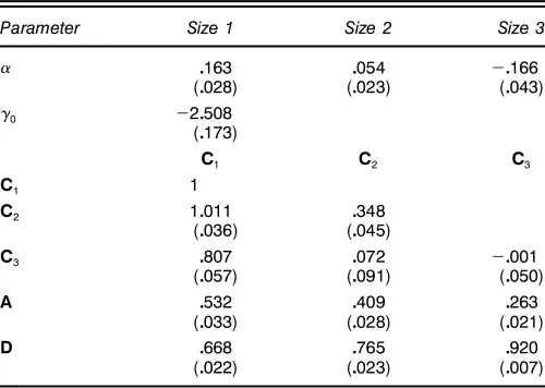
Table 4 reports the results of estimating (23) using Gaussian Q-MLE techniques. We observe some substantial changes in point estimates of the size 1 and size 3 portfolios. The size 1 intercept increases from .108 to .163, whereas the size 3 inter-cept declines fromƒ0004 toƒ0166, a substantial increase in absolute value. Estimates of the conditional covariance matrix appear to be consistent with typical results from estimating GARCH models. All portfolios are signicantly inuenced by both shocks to volatility (A) and memory in volatility (D). We
Table 2. Multivariate Tests of Conditional Normality and Elliptical Symmetry
Size portfolios
Multivariate kurtosis test
Unconditional returns 170054ü
Unconditional residuals 170726ü
Conditional returns 40395ü
Conditional residuals 60167ü
Elliptical symmetric test(Sn)
Conditional returns 10599†
Conditional residuals 0426†
NOTE: The test statistics are Mardia’s (1970) multivariate kurtosis measure and Beran’s (1979) test for elliptical symmetry. Tests are constructed using the series of portfolio returns (rt) and residuals (ut) and where both series are weighted by the matrixH
1=2
t . The
multivari-ate kurtosis measure has been scaled so that assuming normality the statistic will have an asymptotic N(011)distribution.
üIndicates apvalue<001.
†Indicates apvalue>01.
Table 3. OLS Estimation of the Unconditional CAPM
‚i m
Portfolio Estimate Std. error Estimate Std. error
Size 1 0108 0050 0475 0018
Size 2 0032 0049 0659 0018
Size 3 ƒ0004 0004 10031 0001
NOTE: Data are from the CRSP dataset of stocks listed on the NYSE, AMEX, and NASDAQ. Value-weighted returns are calculated daily from January 1996–December 1997. Three size portfolios are created according to the previous day’s market value of equity. The previous day’s NYSE size quartiles are used as the cutoffs for the size portfolios. The CAPM model takes on the parameterizationrtDÁCÂrm1tCut.
do nd that the portfolio of smaller rms are more (less) inu-enced by shocks (memory) than are the portfolios of larger rms. These ndings are again consistent with stylized facts of these models.
Table 5 reports the results of estimating (23) using our semiparametric estimator with the bi-quartic kernel. (Similar results were obtained with the Gaussian kernel and are not reported to save space.) In computing our kernel estimate of the score we make use of Schuster’s (1985) correction. The Appendix provides descriptions of the kernels and of Schus-ter’s correction. We use the Box–Cox transformation with ztD’ 4wt5Dw†tƒ1
† with †D 1
2n in construction of the semi-parametric estimates. This choice of†was found by Hodgson et al. (in press) to yield good results in Monte Carlo experi-ments in a linear model. We also use separate optimal mean integrated squared error (MISE) bandwidth parameters 4‘T5 for estimating ƒ4z5 and ƒ04z5. In estimating the conditional expectationE6bvec4ØtØT
t5—wt7as given by (18), we set the num-ber of draws MD500. Results were not sensitive to larger choices for this number.
Table 4. Q-ML Estimation of the C-CAPM
Parameter Size 1 Size 2 Size 3
0163 0054 ƒ0166
(0028) (0023) (0043)
ƒ0 ƒ20508
(0173)
C1 C2 C3
C1 1
C2 10011 0348
(0036) (0045)
C3 0807 0072 ƒ0001
(0057) (0091) (0050)
A 0532 0409 0263
(0033) (0028) (0021)
D 0668 0765 0920
(0022) (0023) (0007)
NOTE: Data are from the CRSP dataset of stocks listed on the NYSE, AMEX, and NASDAQ. Value-weighted returns are calculated daily from January 1995–December 1997. Three size portfolios are created according to the previous day’s market value of equity. The previous day’s NYSE size quartiles are used as the cutoffs for the size portfolios, as well as for con-struction of weights. The ’rst two quartiles are grouped into the ’rst size portfolio, with the remaining two quartiles each representing the other two portfolios. The C-CAPM takes on the parameterizationrtDÁCexp(ƒ0)Ht×tƒ1Cut, with the scaled conditional variance parame-terizationHtDCCTCAutƒ1uTtƒ1ACDHtƒ1D. Point estimates of the parameters are reported, as are standard errors, which are reported below the point estimates in parentheses.
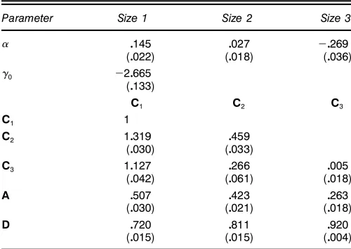
Table 5. Semiparametric Ef’cient Estimation of the C-CAPM
Parameter Size 1 Size 2 Size 3
0145 0027 ƒ0269
(0022) (0018) (0036)
ƒ0 ƒ20665
(0133)
C1 C2 C3
C1 1
C2 10319 0459
(0030) (0033)
C3 10127 0266 0005
(0042) (0061) (0018)
A 0507 0423 0263
(0030) (0021) (0018)
D 0720 0811 0920
(0015) (0015) (0004)
NOTE: Data are from the CRSP dataset of stocks listed on the NYSE, AMEX, and NASDAQ. Value-weighted returns are calculated daily from January 1995–December 1997. Three size portfolios are created according to the previous day’s market value of equity. The previous day’s NYSE size quartiles are used as the cutoffs for the size portfolios, as well as for con-struction of weights. The ’rst two quartiles are grouped into the ’rst size portfolio, with the remaining two quartiles each representing the other two portfolios. The C-CAPM takes on the parameterizationrtDÁCexp(ƒ0)Ht×tƒ1Cut, with the scaled conditional variance
parameter-izationHtDCCTCAutƒ1uT
tƒ1ACDHtƒ1D. Point estimates of the parameters are reported, as are standard errors, which are reported below the point estimates in parentheses. Estimates are obtained using the SE procedure. We report estimates in this table using the bi-quartic kernel and the transformation function’(wt)D(wt†ƒ1)=†.
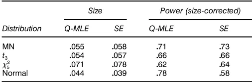
Standard errors tend to fall somewhat when using the semiparametric efcient estimator rather than the Gaussian Q-MLE, and the point estimates ofusing the semiparamet-ric estimator tend to be smaller than for their Q-MLE coun-terparts. The Wald test statistics of the validity of the CAPM, formed from the estimates, are given in Table 6. For the unconditional CAPM, we nd that OLS leads to a marginal rejection of the CAPM at the 5% level. When we look at the tests of the C-CAPM, both estimation methods lead to strong rejections of the model withp values<.01.
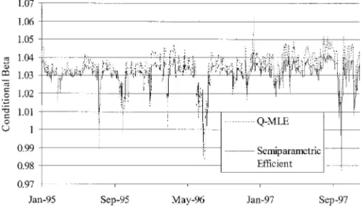
Although the inferences regarding are quite similar for the two methodologies, we nd some potentially interesting differences in the estimated systematic risk as measured by beta 4Ât5. These differences are seen in lists of parameter estimates Tables 4 and 5, or perhaps more easily observed in Figures 1–3. These gures plot the conditional betas for the three portfolios showing the Q-MLE beta as well as the
Table 6. Mean-Variance Ef’ciency Tests
J(pvalue)
Unconditional CAPM
OLS 7095 (005)
C-CAPM
Q-MLE 264011 (<001)
SE 543033 (<001)
NOTE: The test statistics are constructed using the intercepts from estimating the C-CAPM. Mean-variance ef’ciency implies that the intercepts are jointly equal to 0:H02 iD0iD
11 : : : 1n. The table lists the tests that result from estimating the unconditional CAPM model via OLS, the C-CAPM using Q-MLE techniques, as well as the ef’cient procedure using the bi-quartic kernel. Under the null that the C-CAPM is the true model,Jis distributed asymptotically chi-squared (3).
Figure 1. Conditional Beta for the Size 1 Portfolio (- - - Q-MLE; —– SE).
semiparametrically estimated beta using the bi-quartic kernel. We observe that the‚11 t (size 1 portfolio) tends to be higher for the Q-MLE relative to the semiparametric estimates. How-ever, for the other two portfolios, the estimatedÂt is greater for the semiparametric estimator than for the Q-MLE. We also nd that the variability of Ât is greater for the Q-MLE than for the semiparametric estimates. This is true for all of the portfolios, but especially for the size 1 and 2 portfolios. For these, the standard deviation of Ât is 48% smaller for the semiparametric estimate then for the Q-MLE estimate. On the other hand, the standard deviation of ‚31 t is only 2% smaller for the semiparametric estimate.
We also provide graphs of conditional expected returns for the three portfolios. These graphs are found in Figures 4–6. We dene the conditional expected return as
Etƒ1rtD OÁCexp4ƒO05bHt×tƒ10
These graphs incorporate both the intercepts and the condi-tional betas and give a net effect on the parameters of inter-est for our semiparametric efcient method relative to Q-MLE methods. In general, we nd that the semiparametric efcient method leads to estimates of conditional expected return that are greater than those obtained by Q-MLE methods. These differences are small for the size 1 portfolio but increase as
Figure 2. Conditional Beta for the Size 2 Portfolio (- - - Q-MLE; —– SE).
Figure 3. Conditional Beta for the Size 3 Portfolio (- - - Q-MLE; —– SE).
we move to the larger rm portfolios. We observe that the dif-ferences in the estimates of the scaled conditional covariance matrix4Ht5tend to dominate differences in the intercept4Á5. In general, the semiparametric method estimates a larger por-tion of return due to systematic risk and a smaller porpor-tion of return coming from unexplained effects relative to Q-MLE.
6. SIMULATIONS
We simulate series of multivariate GARCH41115time series using the data-generating process
rtDÁCexp4ƒ05Ht×tƒ1Cut1 (24)
with
HtDCC TC
Autƒ1u T tƒ1A0
We setnD2,T D759, and use the parameterizations
CD
µ
1 0
0 1015
¶
1 AD
µ
05 0 0 025
¶
1
and ƒ0D ƒ2075. This simulation setup is a simplication of our empirical model, adopted for the purpose of reduc-ing the computer time required to run the simulations. We
Figure 4. Conditional Expected Return for the Size 1 Portfolio
( Q-MLE; —– SE).
Figure 5. Conditional Expected Return for the Size 2 Portfolio
( Q-MLE; —— SE).
use the same ×tƒ1 from our empirical analysis but reduce the dimension to a 21 vector by combining the smaller two quantile weights into one weight. We also simulate data using two differentÁ vectors,ÁD80109 under the null and ÁD8ƒ0151 0159under the alternative.
We add a randomly selected residual4ut5from some pre-specied distribution. We consider a normal, a mixture of normals, a Studentt with 3 degrees of freedom, and a chi-squared with 5 degrees of freedom. The rst three distri-butions are elliptical, whereas the third is asymmetric and is included as a check on the robustness of our estima-tor to misspecication. To compute the mixture of normals, we rst dene the uniform random variable, U 260117. If U < 41ƒ…5, then letutDpŠ1uMt, where uMt¹N 40115. Oth-erwise, we let ut DpŠ2uMt. The resulting ut will follow a mixed normal distribution. We set …D08 andŠ1D065 in the simulations, and for all distributions the errors are scaled to have unit variances. We use the same residual in construct-ing both the alternative and null series. For each simulation, we estimate (24) using Q-MLE and the semiparametric ef-cient estimator. We replicate each simulation 2,000 times for each distribution and report the results of the simulations in Tables 7–9.
Figure 6. Conditional Expected Return for the Size 3 Portfolio
( Q-MLE; —– SE).
Table 7. Parameter Estimate Results for the Simulation Study
MN t3 52 Normal
Parameter Bias Std. Dev. MSE Bias Std. Dev. MSE Bias Std. Dev. MSE Bias Std. Dev. MSE
0 Q-MLE ƒ0004 0053 0003 ƒ0011 0081 0007 0133 0083 0025 ƒ0015 0050 0003
SE 0005 0052 0003 ƒ0020 0078 0006 0160 0081 0032 0025 0089 0009
1 Q-MLE ƒ0007 0059 0004 ƒ0024 0043 0002 ƒ0162 0072 0031 ƒ0019 0079 0007
SE ƒ0004 0058 0003 ƒ0019 0044 0002 ƒ0160 0074 0031 ƒ0010 0121 0015
ƒ0 Q-MLE ƒ0229 10006 10064 ƒ0431 10169 10552 ƒ0013 10053 10109 ƒ0435 0906 10010
SE ƒ0398 10731 30154 ƒ0497 20404 60026 ƒ0196 10781 30210 ƒ10207 20075 50762
C2 Q-MLE ƒ0017 0235 0056 ƒ0106 0286 0093 ƒ0030 0238 0058 ƒ0011 0187 0035
SE 0015 0223 0050 ƒ0097 0279 0087 0006 0252 0064 0068 0208 0047
A1 Q-MLE ƒ0170 0161 0055 ƒ0106 0259 0078 ƒ0173 0173 0060 ƒ0186 0145 0056
SE ƒ0074 0157 0030 ƒ0076 0251 0068 ƒ0011 0180 0033 ƒ0280 0162 0105
A2 Q-MLE ƒ0129 0119 0031 0086 0216 0054 ƒ0123 0173 0045 ƒ0142 0122 0035
SE ƒ0111 0105 0023 0151 0208 0066 ƒ0082 0167 0034 ƒ0117 0164 0041
NOTE: This table lists the estimation results from a Monte Carlo study. Four different simulations were performed where the residuals were drawn from three different distributions: mixed normal (MN),t3,52, and normal as indicated on the top row. The following parameter values were used in the simulation study:0D1D0,ƒ0D ƒ2050,C2D1015,A1D05, andA2D025. Each series had a length of 759, with 2,000 replications performed for each of the four distributions. Q-MLE and SE methods are used to estimate the model. The bias (average estimated valueƒtrue value), standard deviation of the parameter estimates, and MSE are reported.
Table 7 reports bias, standard deviation, and mean squared error (MSE) for the estimators for the four different distributions. For the nonnormal elliptical densities, the semi-parametric estimator (SE) yields only slight improvements in estimation of the intercepts, with larger improvements found in the estimation of the conditional variance parameters. This is consistent with our empirical study, in which we found that the SE point estimates had greater impact on conditional covariances than on intercepts. Estimation of the risk aversion parameterƒ0 deteriorates when we move from the Q-MLE to the SE, but neither estimator accurately estimates this param-eter. We should point out that for the purposes of this article, ƒ0 is not of substantive interest, because we have focused our attention on testing for zero intercepts and estimating betas, both problems in which ƒ0 can be thought of as a nuisance parameter. Note that in the case of asymmetric errors, the SE provides reasonably good estimates of most of the parameters.
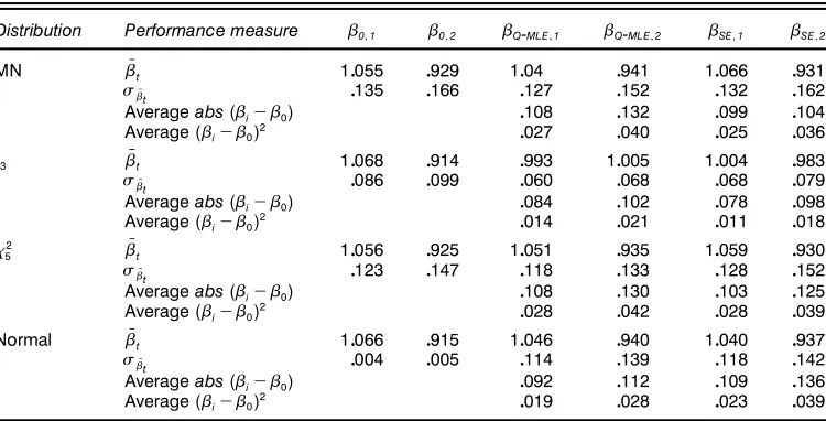
Table 8. Analysis of‚Performance From the Simulation Study
Distribution Performance measure ‚011 ‚012 ‚Q-MLE11 ‚Q-MLE12 ‚SE11 ‚SE12
MN ‚Nt 10055 0929 1004 0941 10066 0931
‘‚Nt 0135 0166 0127 0152 0132 0162
Averageabs(‚iƒ‚0) 0108 0132 0099 0104
Average(‚iƒ‚0)2 0027 0040 0025 0036
t3 ‚Nt 10068 0914 0993 10005 10004 0983
‘‚Nt 0086 0099 0060 0068 0068 0079
Averageabs(‚iƒ‚0) 0084 0102 0078 0098
Average(‚iƒ‚0)2 0014 0021 0011 0018
2
5 ‚Nt 10056 0925 10051 0935 10059 0930
‘‚Nt 0123 0147 0118 0133 0128 0152
Averageabs(‚iƒ‚0) 0108 0130 0103 0125
Average(‚iƒ‚0)2 0028 0042 0028 0039
Normal ‚Nt 10066 0915 10046 0940 10040 0937
‘‚Nt 0004 0005 0114 0139 0118 0142
Averageabs(‚iƒ‚0) 0092 0112 0109 0136
Average(‚iƒ‚0)2 0019 0028 0023 0039
NOTE: This table lists various measures of‚performance of the Q-MLE and the SE estimator. The measure‚Ntis constructed by taking the sample average of‚t for each simulation and then averaging over the simulations. The measure‘‚Nt is constructed by taking the standard deviation of the average‚t’s over the simulations.‚0corresponds with the “true” beta as opposed to estimated beta. The measure averageabs(‚iƒ‚0)is constructed by taking the average absolute difference between the estimated‚tand‚0and then averaging over the simulations. Average(‚iƒ‚0)2reports where squared differences are taken as opposed to absolute differences.
This is important because, recalling our earlier comments, we have no theoretical results on the behavior of the SE under asymmetry, but the simulation results suggest that the SE may be robust to asymmetry. As we would expect, for the case of normal errors we see some deterioration in the performance of the SE conditional mean estimates relative to their Q-MLE counterparts, because the latter are fully efcient maximum likelihood estimates in this case. However, the SE estimates of conditional variance parameters are quite close to their MLE counterparts.
Table 8 compares the simulation results in the estimation of betas. For each simulation, we use the true parameter val-ues and the simulated residuals to construct a time series of “true” betas, Âi
0, where i indexes the simulation. We com-pute the average values ofÂi
0 for each portfolio over the time series as well as the standard deviations of Âi
0, 4‘Âi
01 j5 for
each simulation. We then dene ‚01 j D 210001 P21000
iD1 Â i 01 j and