Vol. 16, No. 2 (2010), pp. 89–104.
ALLELE FREQUENCIES IN MULTIGENE FAMILIES
S. Padmadisastra
Department of Statistics, Universitas Padjadjaran Jalan Raya Bandung Sumedang Km 21 Jatinangor, Indonesia,
s padmadisastra@yahoo.com
Abstract. Results on allelle frequencies in three chromosomes, drawn at random
from a diploid population, evolving in equilibrium, at a particular generation, are presented in this paper. The genes on each chromosome are subject to unbiased and reciprocal gene conversion and mutation. Using the coalescent approach we find the probability distribution of the allelic configurations in the three chromosomes, and the moments of the allelic numbers that exist in one of the three chromosomes or in a pair of chromosomes. We also consider the identity coefficients of two genes drawn at random, one from each of two chromosomes, and the probability that all genes in the three chromosomes are monomorphic. Numerical examples are also given together with simulation results, and they agree well.
Key words and Phrases: Coalescent approach, allelic configurations, identity coeffi-cients, monomorphic probability.
Abstrak.Dalam makalah ini dibahas mengenai frekuensi alel dalam tiga buah
kro-mosom yang diambil secara acak, pada suatu generasi tertentu, dari sebuah populasi diploid. Dianggap bahwa populasi berada dalam keadaan stabil (equilibrium). Gen dalam tiap kromosom dapat mengalami mutasi dan konversi. Menggunakan pen-dekatan koalisi (coalescent) diperoleh distribusi peluang dari konfigurasi alel dalam ketiga kromosom, dan momen-momen mengenai banyak alel yang ada dalam sebuah dan sepasang kromosom. Selain itu diperoleh juga koefisien identitas dari dua buah gen yang diambil secara acak, masing-masing satu dari tiap kromosom, dan pelu-ang bahwa semua gen dalam ketiga kromosom monomorfik. Hasil ypelu-ang diperoleh ternyata sangat sesuai dengan yang diperoleh melalui simulasi.
Kata kunci: Pendekatan koalisi, konfigurasi alel, koefisien identitas, peluang monomorfik.
2000 Mathematics Subject Classification: 62P10. Received: 23-08-2010, accepted: 08-11-2010.
1. Introduction
Watterson [19] studied the joint allelic configurations of two chromosomes in a population. Here we extend his results by considering one more chromosome; thus the object of study here is the joint allelic configuration in three chromosomes. We employ similar techniques to his; namely the “coalescent approach”. In this approach, as we proceed backward in time, two chromosomes coalesce into one class if they are descended from the same ancestor. This approach has been successful in tackling many problems in population genetics; see for instance Griffiths [2], Kingman [5,6], Tavare [14] and Watterson [15, 16] and Kaplan and Hudson [3].
We also use a similar model of evolution; namely that the population follows a Wright-Fisher model, in which each offspring generation is formed through sampling at random with replacement from its parent generation at the end of its life-cycle. Thus generations do not overlap. Here we assume that the population consist of 2Nchromosomes, it evolves in equilibrium and within each chromosome there is a multigene family of n genes. During the formation of a generation, any of then genes in the chromosome might mutate into a novel allele, never before seen, with rateν/2Nper gene per generation. Thus the number of possible alleles is infinite; this is the infinitely many alleles model of Kimura and Crow [4]. It may also happen that during this time one gene, in a chromosome, converts the type of another gene, on the same chromosome, into its type. We let the probability that the ith gene
will convert thejthgene to have its allelic type beλ/2N per generation.
The gene conversions are unbiased and reciprocal. We assume thatν,λ, and nareO(1) and thatN is large so that there is negligible chance of more than one mutation or gene conversion per chromosome per generation. Further, we assume in this model there is no crossing-over.
2. Main Results
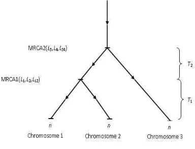
If we trace back the ancestorship of the three sampled chromosomes, drawn at random from a particular generation of a Wright-Fisher model, it may happen that two of them were descended from a “most recent common ancestor” (MRCA1) in some particular generation, a generation more recent than when the whole three were descended from their most recent common ancestor (MRCA2); see Fig. l. Denote by Tl the time between the present and when the first two coalesce into
Figure 1. Chromosome configurations
one class; i.e. the time for their MRCA1, and byT2 the time when these first two, after coalescing into one group, join together with the remaining chromosome into one class. Here time is measured in units of 2N generations.
In Fig. l, we have numbered the two chromosomes that join together first as “1” and “2” and the remaining one, “3.” The symbolsLwill be explained shortly. Of course, in practice, we may not be able to determine which pair of chromosomes diverged most recently; however, for our theoretical results we will assume that this is known.
It can be shown that, in the limit, when 2N → ∞, the approximate joint probability density function of (T1,T2) is
f(t1, t2) = 3e−(3t1+t2) t1≥0, t2≥0 (1)
conditional on “1” and “2” joining first. ThusTlandT2are conditionally indepen-dent and have exponential densities with mean 13 and 1 respectively.
timeT1+ 1, then let us suppose that there areL3andL4founder genes in MRCA2 for Chromosomes 3 and MRCAl, see Fig. 1.
We can consider the genes in the MRCAl and MRCA2 as consisting of four subsets; namely,
(1) the MRCAl genes which, when copied into the two daughter chromosomes, become founder genes in daughter chromosome “1” but not founder genes in daughter chromosome “2”,
(2) those genes which become founder genes in chromosome “2” but not founder genes in chromosome “1”,
(3) those genes which become founder genes in both chromosomes “1” and “2”, (4) those genes in the MRCAl which do not become founder genes in either
daughter chromosome.
A similar description as above can be given for MRCA2, but to save space we omit it.
We writeL12for the number of MRCAl genes in the third subset. Then the four subsets are of sizesL1−L12, L2−L12, L12andn−L1−L2+L12respectively. Similarly we writeL34for the number of MRCA2 genes which are founders for both Chromosome 3 and MRCAI genes. Then the four subsets of MRCA2 are of sizes L3−L34, L4−L34, L34andn−L3−L4+L34 respectively.
Of course, in the present situation, the statement that the evolution of a chromosome is mathematically equivalent to the evolution of a population of n genes in Moran’s model, proved by Watterson [18] under Shimizu’s [12] model for the evolution of multigene families, will also hold. Thus the conditional distribution of the numbers of founder genes, L, which are ancestors forn, non-mutant genes at timeT later, is
P(L=l|T =t, n) =ql(t, n), (2)
where
ql(t, n) = n
X
j=l
e−λj+(j+θ−1)ta(j, l, n) l= 0, . . . , n, (3)
and forj >0,
a(j, l, n) = (−1)j−l(2j+θ−1)(l+θ)(j−1)n[j] l!(j−l)!(n+θ)(j)
(4)
while for j = 0, a(0,0, n) = 1. In the above formula, we use the ascending and descending factorial notations;
θ(j)=θ(θ+ 1)· · ·(θ+j−1),and θ[j]=θ(θ−1)· · ·(θ−j+ 1).
LetL = (L1, L2, L12, L3, L4, L34), T= (T1, T2) and P(l|T) denote the pro-bability thatL has valuelgivenT. AveragingP(l|t) with respect to (1), we have the joint unconditional distribution ofL, P(l),
P(l) = 3h(l1, l2, l12)h(l3, l4, l34),
Now to describe the joint allelic configurations in the three chromosomes, let Γj1,j2,j3 denote the number of alleles each represented by j1, j2 and j3 genes in our sampled chromosomes, respectively. We obtain the p.g.f. for the trivariate frequency spectrum,{Γj1,j2,j3}, of the three sampled chromosomes
where the sum over i means the sum overi1, i2, i3, and i4, withi1+i2+i3 ≥1 and the sum over j means the sum overj1 ≥i1, j2 ≥i2, and j3 ≥i3. It can be shown that the p.g.f. is correctly normalized.
3. Applications
3.1. Trivariate Frequency Spectrum. Differentiating (6) with respect toVj1,j2,j3 and then putting allV’s equal to 1 yieldsE(Γj1,j2,j3). After some algebra, we found, the following relations hold,
X
chromosomes would be identical. Let ˆI2 ( ˆI3) denote the probability of the event in the two (three) chromosomes, then
ˆ
Equations (9) and (10) are obtained using similar reasoning as in the two chromosomes case of Watterson [19], except that in the three chromosomes case, the probability that two genes drawn at random from two randomly chosen chro-mosomes, ˆI2 or ˆI in Watterson’s notation, now is the average of the probabilities calculated for different pairs of chromosomes “1” and “2”, or “1”and “3”.
3.3. Numbers of Alleles. The number of alleles that exist in one, in a pair, or in all three sampled chromosomes can be expressed in terms of frequency spectrum I’j1,j2,j3. We write
for the numbers of alleles in the first, second and third sampled chromosome. Let the number of alleles that exist on both chromosome 1 and 2 beK12on 1 and 3 be K13, and on 2 and 3 beK23. Then
Clearly the number of alleles that exist in all three chromosomes,K123 say, is
assignment is done according to the definition of K’s given above. Thus into (6)
To find the p.g.f ofK, the total number of alleles present in at least one of the three chromosomes, putS1=S2=S3=S123=S andS12=S13=S23=S−1,
In turns out that,
E(SK) = (11)
The above result shows thatK may be written as a sum of independent Bernoulli random variables, givenL=l; i.e.,
K = (X1n+X1n−1+· · ·+X1l1 +1) + (X2n+X2n−1+· · ·+X2l2 +1) (12)
The interpretation of these variables is that X1j, and X2j, denote the numbers
(0 or 1) of mutations which occur during T1 in chromosomes 1 and 2, while X3j,
mutations occur duringT1+T2 in chromosome 3, and because of the model, these mutations will produce new alleles which exist only in one chromosome but not in the other two, respectively. Those that founded both chromosomes 1 and 2 but arose as mutants duringT2 are represented byX4j, and similiarlyX5j, represents
To find moments of K we can use either (11) or (12). Either way we find but the most interesting case is perhaps when k = 1. This will give the proba-bility that all the genes in the three chromosomes have only one type. i.e. are monomorphic. Thus from (11)
Pmono = P(K= 1) =P(K1=K2=K3=K12=K13=K23=K123= 1)
We can interpret the meaning of the terms in the above expression as follows. The first factorθis saying that the one allelic type arose by mutation at some time. The second factor, (nθ−1)!
n , is related to Ewens’ sampling formula; i.e. θ(n−1)!
θn is the
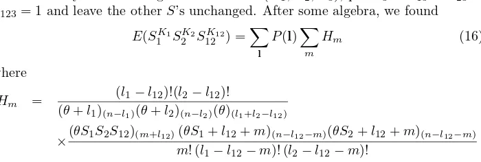
To study the the marginal behavior of (K1, K2, K3), put S3 =S13=S23 = S123= 1 and leave the otherS’s unchanged. After some algebra, we found
E(SK1
1 S K2
2 S K12
12 ) =
X
l
P(l)X
m
Hm (16)
where
Hm =
(l1−l12)!(l2−l12)!
(θ+l1)(n−l1)(θ+l2)(n−l2)(θ)(l1+l2−l12)
×(θS1S2S12)(m+l12)(θS1+l12+m)(n−l12−m)(θS2+l12+m)(n−l12−m) m! (l1−l12−m)! (l2−l12−m)!
In the calculation of the moments, other thanE(K1) and Var(K1), we have to useP(l) as in (eq5) because the marginal distribution of (L1, L2, L12) obtain by summing outL3,L4, andL34 is not the same as distribution of (L1, L2, L3) in the two chromosomes case of Watterson [19]. Perhaps the mere knowledge that there is a Chromosome “3” older than “1” and “2”, means that “1” and “2” are not randomly chosen.
Further, by putting allS’s equal to 1 exceptS3 =S, it can be shown what the p.g.f of K3 equals
E(SK3) = (θS)(n) θ(n)
Thus the number of distinct alleles in Chromosome 3 also follows Ewens’ sampling formula.
It is rather unfortunate that we can not exploit (6) any further; in particular we are not able to simplify any other p.g.f. that involves Chromosome 3, such as the marginal p.g.f. E(SK1
1 S K3
3 S K13
13 ) etc. But Chromosome 3’s behaviour still can be studied through simulation.
4. Discussion and Examples
In this section we present some numerical example of the results obtained ear-lier together with some simulation results. The simulation is done using Watterson’s method of simulation, Watterson [16,17,18,19]. In each replicate of simulation we produce three families of gene each of sizenand all the simulation results presented here are obtained from 10000 replicates. Throughout the tables, the simulation re-sult are given in parentheses. In general, in all of the tables, the simulation rere-sults agree very closely with the results calculated from the theoretical formulas, except in some entries where the latter are not available.
are explained in Section 3.3. as they should be, the values of E(K1) and Var(K1) are exactly the same with those in Table I of Watterson [19]. Other features of the table are also similar to that found in the two chromosomes case; namely keeping the mutation parameter fixed at ν = 0.2 and increasing the values ofθ produces larger number of alleles in each chromosomes. While keepingθconstant atθ= 0.45 and varying the values ofν does not produce any effect; the marginal moments are constant for different values of ν. The numerical results on the joint behavior of
Table I. Alleles in One Chromosomes Moments ofK1, K2 andK3
n θ E(K1) Var(K1)
ν = 0.2, throughout,θ=ν/λ
2
0.045 1.0431 (1.0466) 0.0412 (0.0444) 0.09 1.0826 (1.0824) 0.0758 (0.0756) 0.225 1.1837 (1.1826) 0.1499 (0.1493) 0.45 1.3103 (1.3080) 0.2140 (0.2132)
5
0.045 1.0910 (1.0960) 0.0883 (0.0904) 0.09 1.1768 (1.1754) 0.1668 (0.1652) 0.225 1.4078 (1.4072) 0.3562 (0.3556) 0.45 1.7256 (1.7269) 0.5683 (0.5692)
10
0.045 1.1243 (1.1245) 0.1214 (0.1192) 0.09 1.2429 (1.2442) 0.2320 (0.2381) 0.225 1.5699 (1.5762) 0.5128 (0.5239) 0.45 2.0392 (2.0409) 0.8615 (0.8539)
θ= 0.45 throughout
10 0.02 2.3092 (2.0506) 0.8615 (0.8679) 0.2 2.3092 (2.0409) 0.8615 (0.8463) 2.0 2.3092 (2.0453) 0.8615 (0.8651)
λ= 0.44 throughout
10 0.02 1.1255 (1.1236) 0.1225 (0.1201) 0.2 2.0479 (2.0512) 0.8674 (0.8493) 2.0 5.6473 (5.6391) 2.0359 (2.0365)
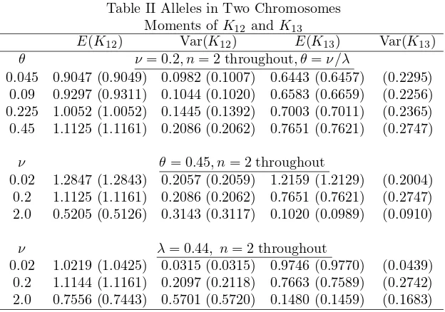
two chromosomes can be seen in Table II. In this table the moments of the number of common alleles between chromosomes 1 and 2,K12, and between Chromosomes 1 and 3, K13 are given. E(K13) is found from K13 =Pj1=1
P
j2=0 P
Table II Alleles in Two Chromosomes Moments ofK12 andK13
E(K12) Var(K12) E(K13) Var(K13) θ ν = 0.2, n= 2 throughout, θ=ν/λ
0.045 0.9047 (0.9049) 0.0982 (0.1007) 0.6443 (0.6457) (0.2295) 0.09 0.9297 (0.9311) 0.1044 (0.1020) 0.6583 (0.6659) (0.2256) 0.225 1.0052 (1.0052) 0.1445 (0.1392) 0.7003 (0.7011) (0.2365) 0.45 1.1125 (1.1161) 0.2086 (0.2062) 0.7651 (0.7621) (0.2747)
ν θ= 0.45, n= 2 throughout
0.02 1.2847 (1.2843) 0.2057 (0.2059) 1.2159 (1.2129) (0.2004) 0.2 1.1125 (1.1161) 0.2086 (0.2062) 0.7651 (0.7621) (0.2747) 2.0 0.5205 (0.5126) 0.3143 (0.3117) 0.1020 (0.0989) (0.0910)
ν λ= 0.44, n= 2 throughout
0.02 1.0219 (1.0425) 0.0315 (0.0315) 0.9746 (0.9770) (0.0439) 0.2 1.1144 (1.1161) 0.2097 (0.2118) 0.7663 (0.7589) (0.2742) 2.0 0.7556 (0.7443) 0.5701 (0.5720) 0.1480 (0.1459) (0.1683)
former were descended from a more recent common ancestor than Chromosomes 1 and 3 did. Another noteworthy feature is that the values ofE(K12) are generally higher than those ofE(K12) in the two chromosomes case (Watterson [19]) but the opposite happens toE(K13); i.e. its values are smaller. The effect of the parameter values on their joint behaviour is similar to that in the two chromosomes case.
We also note a relationship betweenE(K12),E(K13),E(K23) in our results withE(K12) in Watterson [19]. Their relationship can be formulated as
E(Watterson’sK12) = 1
3(E(K12+E(K13+E(K23)
= 1
3E(K12) + 2
3E(K13)
For example, whenν = 0.2,n= 2 andθ= 0.045, from Table III of Watterson [19], we see E(K12) = 0.731. This exactly the average ofE(K12),E(K13), and E(K23) given in our Table II for same parameter values.
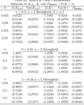
The behaviour of the number,K123, of the alleles common to the three chro-mosomes, the number, K, of alleles altogether, and the probability that all alleles in all the three chromosomes are of one allelic type, are given in Table III. The ex-pected number of alleles in common to all three chromosomes,E(K123), is obtained from the relationK123=Pj1=1
P
j2=1 P
Tabel III. Alleles in Three Chromosomes Moments ofK123,K, andPmono =P(K= 1) θ E(K123) Var(K123) E(K) Var(K) Pmono
ν= 0.2,n= 2 throughout,θ=ν/λ
0.045 0.6123 – 1.5483 0.4458 0.5435 (0.6116) (0.2378) (1.5514) (0.4470) (0.5420) 0.09 0.6266 – 1.6280 0.5274 0.5032
(0.6334) (0.2338) (1.6234) (0.5268) (0.5074) 0.225 0.6653 – 1.8105 0.6946 0.4175
(0.6633) (0.2444) (1.7955) (0.6817) (0.4250) 0.45 0.7237 – 2.0121 0.8395 0.3304
(0.7163) (0.2800) (2.0191) (0.8420) (0.3270)
ν θ= 0.45, n= 2 throughout
0.02 1.2051 – 1.4196 0.3230 0.6183 (1.2011) (0.1949) (1.4242) (0.3235) (0.6135) 0.2 0.7273 – 2.0121 0.8395 0.3304
(0.0772) (0.2800) (2.0191) (0.8420) (0.3270) 2.0 0.0815 – 3.2881 1.0805 0.0321
(0.0772) (0.0722) (3.2957) (1.0856) (0.0307)
ν λ= 0.44, n= 2 throughout
0.02 0.9682 – 1.1275 0.1248 0.8791 (0.9691) (0.0477) (1.1243) (0.1209) (0.8817) 0.2 0.7248 – 2.0153 0.8415 ) 0.3290
(0.7120) (0.2781) (2.0248) (0.8385) (0.3245) 2.0 0.1158 – 4.5232 1.2572 0.0049
(0.1108) (0.1277) (4.5388) (1.2892) (0.0046)
are varied, the number of alleles expected on each chromosome remains constant while the number of alleles in common to two and three chromosomes decreases and the total number of alleles increases, as we expect. Holding λ fixed and in-creasing uhas the same effect as above except that the number of alleles in each chromosome is not constant. Another obvious feature is that the number of alleles in common to all three chromosomes is always smaller than those in common to two chromosomes.
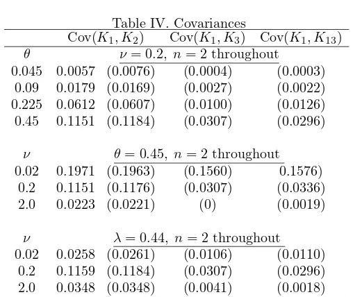
All the entries in Table IV are obtained from simulation, except those of covariances between the number of alleles in Chromosomes 1 and 2, Cov(K1,K2). To save space, not all of the results found for Table IV are presented here. But the discussion given here are based on all the results found. Since theHmterm in (16)
Table IV. Covariances
Cov(K1, K2) Cov(K1, K3) Cov(K1, K13) θ ν = 0.2, n= 2 throughout
0.045 0.0057 (0.0076) (0.0004) (0.0003) 0.09 0.0179 (0.0169) (0.0027) (0.0022) 0.225 0.0612 (0.0607) (0.0100) (0.0126) 0.45 0.1151 (0.1184) (0.0307) (0.0296)
ν θ= 0.45, n= 2 throughout 0.02 0.1971 (0.1963) (0.1560) 0.1576)
0.2 0.1151 (0.1176) (0.0307) (0.0336) 2.0 0.0223 (0.0221) (0) (0.0019)
ν λ= 0.44, n= 2 throughout 0.02 0.0258 (0.0261) (0.0106) (0.0110)
0.2 0.1159 (0.1184) (0.0307) (0.0296) 2.0 0.0348 (0.0348) (0.0041) (0.0018)
different probability terms. Perhaps the most interesting feature of this table is the change from negative to positive covariances, in particular between the number of alleles in common to two chromosomes and the total number of alleles. The total number of alleles among the three chromosomes includes the alleles common to both Chromosomes 1 and 2. Thus one would expect a positive correlation between K andK12. But whenθ is low we expect little diversity, and perhaps the number of common alleles tends to inhibit the number of non-common alleles sufficiently to produce a negative correlation.
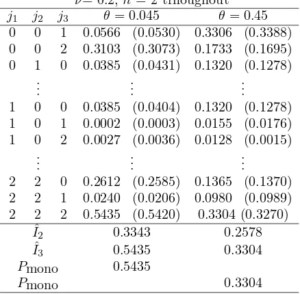
Tabel V Trivariate Frequency Spectrum Γj1,j2,j3 ν= 0.2,n= 2 trhoughout
j1 j2 j3 θ= 0.045 θ= 0.45 0 0 1 0.0566 (0.0530) 0.3306 (0.3388) 0 0 2 0.3103 (0.3073) 0.1733 (0.1695) 0 1 0 0.0385 (0.0431) 0.1320 (0.1278)
..
. ... ...
1 0 0 0.0385 (0.0404) 0.1320 (0.1278) 1 0 1 0.0002 (0.0003) 0.0155 (0.0176) 1 0 2 0.0027 (0.0036) 0.0128 (0.0015)
..
. ... ...
2 2 0 0.2612 (0.2585) 0.1365 (0.1370) 2 2 1 0.0240 (0.0206) 0.0980 (0.0989) 2 2 2 0.5435 (0.5420) 0.3304 (0.3270)
ˆ
I2 0.3343 0.2578
ˆ
I3 0.5435 0.3304
Pmono 0.5435
Pmono 0.3304
itself, two alleles with one representative gene each is more likely than one allele with two representatives.
Acknowledgement. I thank jurusan Statistika, Fmipa – Unpad, for their gener-ous support.
References
[1] Ewens, W. J., ”The Sampling Theory of Selectively Neutral Alleles”,Theor. Pop. Biol. 3
(1972), 87-112.
[2] Griffiths, R. C., ”Lines of Descent in the Diffusion Approximation of Neutral Wright-Fisher Models”,Theor. Pop. Biol.17(1980), 37-50.
[3] Kaplan, N. L. and Hudson, R. R., ”On the Divergence of Genes. I. Multigene Families ”,
Theor. Pop. Biol.31(1987), 178-194.
[4] Kimura, M. and Crow, J. F., ”The Number of Alleles that can be Maintained in a Finite Population”,Genetics49(1964), 725-738.
[5] Kingman, J. F. C., ”On Genealogy of Large Populations”, J. Appl. Prob. A19(1982a), 27-43.
[6] Kingman, J. F. C., ”The Coalescent”,Stoch. Proc. Appl.13(1982b), 235-248.
[7] Nagylaki, T. and Barton, N., ”Intrachromosomal Gene Conversion, Linkage, and the Evolu-tion of Multigene Families”, ”,Theor. Pop. Biol.29(1986), 407-437.
[8] Ohta, T., ”On the Evolution of Multigene Families”,Theor. Pop. Biol.23(1983), 216-240.
[10] Ohta, T., ”Actual Number of Alleles Contained in a Multigene Family”, Genet. Res. 48
(1986), 119-123.
[11] Ohta T., ”Some Models of Gene Conversion for Treating the Evolution of Multigene Families and Other Repetitive DNA Sequenes”, in Stochastic models in Biology ( M. Kimura, G. Kallianpur, T. Hida, Eds. )Theor. Pop. Biol.23(1987), 216-240.
[12] Shimizu, A., Stationary Distribution of a Diffusion Process Taking Values in Probability Distributions on the Partitions, in Stochastic models in Biology ( M. Kimura, G. Kallianpur, T. Hida, Eds. ) Springer-Verlag Berlin, 1987.
[13] Tavare. S., ”Lines of Descent and Genealogical Processes, and Their Applications in Popula-tion Genetics Models”,Theor. Pop. Biol.26(1984), 119-164.
[14] Watterson, G. A., ”Lines of Descent and the Coalescent”, Theor. Pop. Biol. 26(1984a), 77-92.
[15] Watterson, G. A., ”Allele Frequencies after a Bottleneck”, Theor. Pop. Biol.26 (1984b), 387-407.
[16] Watterson, G. A., ”Genetic Divergence of Two Populations”,Theor. Pop. Biol.27(1985a),
298-317.
[17] Watterson, G. A.,Estimating Species Divergence Times using Multilocus Data, in Population Genetics and Molecular Evolution ( T. Ohta and K. Aoki, Eds. ) Springer-Verlag Berlin,1985b. [18] Watterson, G. A., ”Allele Frequencies in Multigene Families . I. Diffusion Equations
Ap-proach”,Theor. Pop. Biol.35(1989a), 142-160.
[19] Watterson, G. A., ”Allele Frequencies in Multigene Families . II. Coalescent Approach”,