Abstract. An alternative to the Parkes’ approach [SIGMA 4 (2008), 053, 17 pages] is suggested for the solutions categorization to the extended reduced Ostrovsky equation (the exROE in Parkes’ terminology). The approach is based on the application of the qualitative theory of differential equations which includes a mechanical analogy with the point particle motion in a potential field, the phase plane method, analysis of homoclinic trajectories and the like. Such an approach is seemed more vivid and free of some restrictions contained in [SIGMA 4(2008), 053, 17 pages].
Key words: reduced Ostrovsky equation; mechanical analogy; phase plane; periodic waves; solitary waves, compactons
2000 Mathematics Subject Classification: 35Q58; 35Q53; 35C05
1
Introduction
In paper [1] E.J. Parkes presented a categorization of solutions of the equation dubbed the extended reduced Ostrovsky equation (exROE). The equation studied has the form
∂
with p, q, and β being constant coefficients. This equation was derived from the Hirota– Satsuma-type shallow water wave equation considered in [2] (for details see [1]).
For stationary solutions, i.e. solutions in the form of travelling waves depending only on one variable χ=x−V t−x0, this equation reduces to the simple third-order ODE:
where V stands for the wave speed andw=u−V. (Note, that in many contemporary papers including [1] authors call such solutions simply “travelling-wave solutions”. Such terminology seems not good as nonstationary propagating waves also are travelling waves. The term “sta-tionary waves” widely used earlier seems more adequate for the waves considered here.) In paper [1], equation (2) was reduced by means of a series of transformations of dependent and independent variables to an auxiliary equation whose solutions were actually categorized subject to some restrictions on the equation coefficients, viz.:
p+q 6= 0, qV −β 6= 0
avoiding any redundant transformations of variables. The method used is based on the phase plane concept and analogy of the equation studied with the Newtonian equation for the point particle in a potential field. Such approach seems more vivid and free of aforementioned re-strictions. This work can be considered also as complementary to paper [1] as the analysis presented may be helpful in the understanding of basic properties of stationary solutions of equation (2).
2
Mechanical analogy, potential function
and phase-plane method
Equation (2) can be integrated once resulting in
w d
where C1 is a constant of integration. By multiplying this equation by dw/dχ and integrating
once again, the equation can be reduced to the form of energy conservation for a point particle of unit mass moving in the potential fieldP(w):
1
where the effective “potential energy” as a function of “displacement” w is
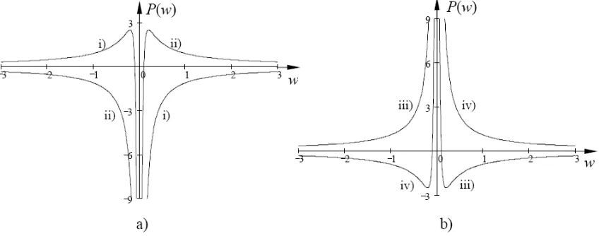
P(w) = p+q
the “potential energy”, P(w). As follows from equation (4), real solutions can exist only for
E ≥P(w). Various cases of the potential function (5) are considered below and corresponding bounded solutions are constructed. Unbounded solutions are not considered in this paper as they are less interesting from the physical point of view; nevertheless, their qualitative behavior becomes clear from the general view of corresponding phase portraits.
3
Particular case:
p
+
q
= 0
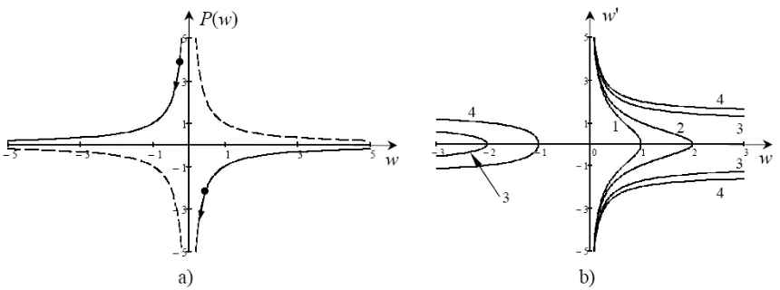
Figure 1. a) Potential function for the casep+q= 0,C2= 0 and two values ofC1: C1= 1 (solid lines),
andC1=−1 (dashed lines). Two dots illustrate possible motions of point particles in the potential field.
b) Phase plane corresponding to the potential function with C1 = 1 and different values ofE. Line 1:
E=−1; line 2: E=−0.5; lines 3: E= 0.5; lines 4: E= 1.
potential function (5) simplifies in this case. However, a variety of subcases can be distinguished nevertheless even in this case depending on the coefficients C1 and C2. All these subcases are
studied in detail below.
3a. If C2 = 0, the potential function represents a set of antisymmetric hyperbolas located either in the first and third quadrants or in the second and fourth quadrants as shown in Fig.1a. The corresponding phase plane (w, w′), where w′ =dw/dχ, is shown in Fig.1b for C
1 = 1 (for C1 = −1 the phase plane is mirror symmetrical with respect to the vertical axis). For other values of C1 phase portraits are qualitatively similar to that shown in Fig. 1forC1 = 1.
Analysis of the phase portrait shows that there are no bounded solutions for any positiveE; corresponding trajectories both in the left half and right half of the phase plane go to infinity onw(see, e.g., lines 3 and 4 in Fig.1b). Meanwhile, solutions bounded onwdo exist for negative values of E (i.e. for V > −β/p), but they possess infinite derivatives when w = 0. Consider, for instance, motion of an affix along the line 2 in Fig. 1b (C1 = 1) from w′ =∞ towards the
axiswwherew′ = 0. The qualitative character of the motion becomes clear if we interpret it in terms of “particle coordinate” w and “particle velocity”w′ treating ξ as the time. The motion originates at some “time”ξ0 with infinite derivative and zero “particle coordinate”w= 0. Then,
the “particle coordinate” w increases to some maximum value wmax =−C1/E (E < 0) as the
“particle velocity” is positive. Eventually it comes to the rest having zero derivative w′ = 0 and w = wmax. Another independent branch of solution for the same value of E corresponds
to the affix motion along the line 1 from the previously described rest point at axis w towards
w′ =−∞ and w= 0.
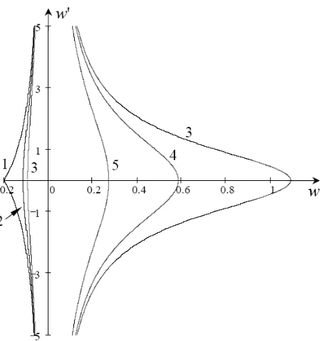
All bounded analytical solutions for this case can be presented in the universal implicit form:
ξ(y)−ξ0=±
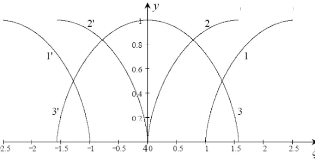
solution consists of two independent branches which correspond to signs plus or minus in front of the square brackets in equation (6). Each branch is defined only on a compact support of axis ξ: either on −π/2 ≤ ξ −ξ0 ≤ 0 or on 0 ≤ ξ−ξ0 ≤ π/2 (see lines 1 and 1′ in Fig. 2).
With the appropriate choice of constantsξ0 one can create a variety of different solutions, e.g.,
Figure 2. Various particular solutions described by equation (6).
Figure 3. Maximum of the compacton solution (6) against speed in the original variables, equation (7). Dashed vertical line corresponds to the limiting value of V =−β/p. The plot is generated forC1=p=
β = 1.
solutions and their independency of each other, one can create periodic or even chaotic sequences of compactons randomly located on axis ξ.
The maximum of the functiony(ξ), ymax= 1, corresponds in terms of wtowmax=−C1/E.
Using the relationship betweenwand the original variableu(see above), as well as the definition of the constant E, one can deduce the relationship between the wave extreme value (wave maximum) and its speed:
umax=V − C1
E =V +
2C1
pV +β. (7)
Taking into account that we consider the case of C1 = 1, and negative values ofE are possible
only when V >−β/p, the plot of umax(V) is such as presented in Fig.3.
As follows from equation (7), a wave is entirely negative (umax<0), when
V < 1
2p
p
β2−8pC1−β,
provided thatp < β2/(8C
1). At greater values ofV, the wave profile contains both positive and
negative pieces, and for certain value of V the total wave “mass” I =R
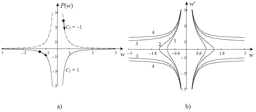
Figure 4. a) Potential function for the casep+q= 0,C1= 0 and two values ofC2: C2= 1 (solid lines),
andC2=−1 (dashed lines). Two dots illustrate possible motions of point particles in the potential field. b) Phase plane corresponding to the potential function with C2 = 1 and different values ofE. Line 1:
E =−1; line 2: E =−0.5; lines 3: E = 0.5; lines 4: E = 1. All lines are symmetrical with respect to axis w′ and are labelled only in the left half of the phase plane.
3b. A similar analysis can be carried out for the case when C1 = 0, C2 6= 0. The potential
function in this case represents a set of symmetric quadratic hyperbolas located either in the first and second quadrants or in the third and fourth quadrants as shown in Fig.4a forC2 =±1. The
corresponding phase plane is shown in Fig. 4b for C2 = 1 only (there are no bounded solutions
for C2 =−1, therefore this case is not considered here). For other positive values of C2 phase portraits are qualitatively similar to that shown in Fig.4b.
Analysis of the phase portrait shows that there are no bounded solutions for C2 = −1, as
well as for C2 = 1 and any positiveE (see, e.g., lines 3 and 4 in Fig.4b); they exist however for C2 = 1 and negative values of E, but possess infinite derivatives at some values of χ. In nor-malized variablesy = (−E/C2)1/2w,ξ =−E(2/C2)1/2χ all possible solutions can be presented
in terms of independently chosen function branches describing a unit circle in one of the four quadrants, i.e.
(ξ−ξ0)2+y2= 1, (8)
where ξ0 is an arbitrary constant of integration.
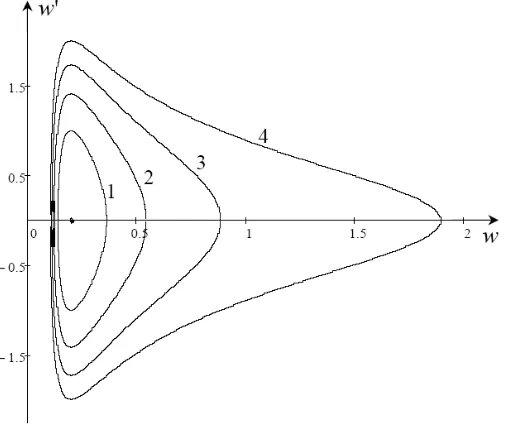
Playing with the constant ξ0 one can create again a variety of compacton-type solutions
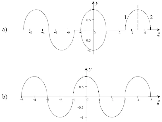
including multi-valued solutions. Some examples of solitary compacton solutions are shown in Fig.5a; they includeN-shaped waves, multi-valued circle-shaped waves and semicircle positive-polarity pulses (due to symmetry, the positive-polarity of the first and last waves can be inverted). In addition to those, various periodic and even chaotic compound waves can be easily constructed; one of the possible examples of a periodic solution is shown in Fig.5b. Each positive or negative half-period of any wave consists of two independent branches originating at y = 0 and ending at y = ±1. The same is true for the pulse-type solutions shown in Fig. 5a; they consist of independent symmetrical branches as shown, for example, for the semicircle pulse in Fig. 5a where they are labelled by symbols 1 and 2.
The maximum of the functiony(ξ), ymax = 1, corresponds in terms of w to the wave
Figure 5. a) Some examples of pulse-type waves described by equation (8): N-shaped wave; circle wave and semicircle compacton. b) One of the examples of a periodic wave with infinite derivatives aty= 0,
ξ= 2n+ 1, wherenis an entire number.
As follows from equation (9), wave maximum (minimum) cannot be less than the certain value, Umax (−Umin), which occurs at some speed V1, where
For all possible values of wave maximum umax > Umax, two values of wave speed are pos-sible, i.e. two waves of the very same “amplitude” can propagate with different speeds. This is illustrated by horizontal dashed line in Fig.6 drawn forumax= 2.5. The same is true for waves
of negative polarity.
3c. Consider now the case when both C1 and C2 are nonzero butp+q is still zero. There
are in general four possible combinations of signs of the parameters C1 and C2:
i) C1 >0, C2>0; ii) C1 <0, C2>0; iii) C1 >0, C2 <0; iv)C1 <0, C2 <0.
The shape of the potential function P(w) and corresponding solutions are different for all these cases. However, among them there are only two qualitatively different and independent cases, whereas the two others can be obtained from those two cases using simple symmetry reasons. This statement is illustrated by Fig. 7, where the potential relief is shown for all four aforementioned cases i)–iv).
Figure 6. Dependence of the wave maximum on speed in original variables, equation (9), as follows from solution (8). Dashed vertical line corresponds toV =−β/p. The plot is generated forC2=p=β = 1.
Figure 7. Potential relief for the four different cases, i)–iv), of various signs of constants C1 and C2.
The plot was generated forC1=±1,C2=±0.1.
operation, i.e. wi) =−wii),wiii)=−wiv). Therefore, below only two qualitatively different cases are considered in detail, namely the cases i) and iii).
Case i) is characterized by an infinite potential well at the origin,w = 0. This singularity in the potential function corresponds to the existence of a singular straight line w = 0 on the phase plane (see Fig. 8). On both sides from this singular line there are qualitatively similar trajectories which correspond to bounded solutions having infinite derivatives at the edges. Quantitative difference between the “left-hand side solutions” and “right-hand side solutions”, apart of their different polarity, is the former solutions (of negative polarity, w ≤0) exist for
E ≤Pmax, whereas the latter ones (of positive polarity, w≥0) exist for E ≤0. The potential
function has a maximum Pmax=C12/(4C2) atw=−2C2/C1. There are no bounded solutions
forE > Pmax.
Consider first bounded solutions which correspond to trajectories shown in the left half-plane,w≤0, in Fig.8. For a positive value of the parameterE in the range 0≤E ≤Pmax, the
analytical solution can be presented in the form
ξ(y) =±2pQ
" p
(y+ 2Q)2−4Q(Q−1)−2Qlny+ 2Q+
p
(y+ 2Q)2−4Q(Q−1)
2p
Q(Q−1)
#
,(10)
Figure 8. Phase portrait of equations (3), (4) for the case i) (only those trajectories are shown which correspond to particle motion within the potential well in Fig. 7a). Line 1: E = 2.5; line 2: E = 1; lines 3: E=−1; line 4: E=−2; line 4: E=−5.
The range of variability onξ is:
|ξ| ≤4Qn1−pQlnh pQ+ 1
/pQ−1io,
whereas y varies in the range
−2hQ−pQ(Q−1)i≤y≤0.
The relationship between the wave minimum and its speed is:
umin=V + with the appropriate choice of the integration constant reduces to
The range of variability on ξ is: |ξ| ≤ 4/3, whereas y varies in the range: −1 ≤y≤0. The relationship between the wave minimum and its speed is also very simple as both of them are again constants but different from those given by equation (14); in this case they are:
V =−β
Bounded solutions corresponding to the trajectories shown in the right half-plane in Fig.8
with w ≥0, exist only for negative E; they are given by equation (12), but with the different range of variability of y: 0 ≤ y ≤ 2h−Q+p
Q(Q−1)i. The relationship between the wave maximum and its speed is given again by equation (11) whereumaxshould be substituted instead
of umin andpV +β >0 as E <0 for these solutions.
Solutions (10), (12), (13) and (15) are shown in Fig.9. All these solutions are of the com-pacton type; they consist of two independent branches which can be matched differently or unmatched at all. Lines 2 and 2′ represent an example when two branches are matched so that they form a semi-oval; lines 3 and 3′ represent another example when two branches are matched so that they form an inverted “seagull”. On the basis of these “elementary” solutions, various complex compound solutions can be constructed including periodic or chaotic stationary waves. The dashed line 1 in the figure corresponds toE= 0 (Q= 8). Another branch of the solution with the same value ofE = 0 represents a solution of positive polarity which is unbounded both on ξ andy. For positive values ofE, solutions of negative polarity become wider and of greater “amplitude” (see line 2). WhenE further increases and approachesPmax, the solution becomes
infinitely wide, but its minimum goes to −2. In the limiting case E = Pmax (Q = 1) two
independent branches of the solution can be matched differently as shown by dashed-dotted lines 3 and 3′ in Fig. 9. The solution vanishes in this case whenξ = 0 and goes to −2 when ξ → ±∞; this situation is described by equation (13).
For the negative E there are two families of solutions: negative one, corresponding to the left-hand side trajectories in Fig. 8, and positive one, corresponding to the right-hand side trajectories. When E, being negative, increases in absolute value (Q varies from −∞ to 0−), solutions depart from the line 1 in Fig. 9 and gradually squeeze to the origin (see line 4 for instance). For the same values of negative E, positive solutions originated at infinity also gradually shrink and collapse in the origin (lines 6 and 5 demonstrate this tendency).
Consider now the case iii) shown in Fig.7b. The potential function in this case has only one well of a finite depth so thatPmin=C12/(4C2) atw=−2C2/C1, whereC2is negative now. There
are no bounded solutions for negative w; they exist however for positivewand E varying in the range Pmin ≤E <0. The finite value of the potential minimum corresponds to the equilibrium
Figure 9. Various solutions described by equations (10), (12), (13) and (15). Compactons of negative polarity: line 1: Q=∞; lines 2 and 2′: Q= 2; lines 3 and 3′: Q= 1: line 4: Q=−0.1. Compactons of positive polarity: line 5: Q=−0.1; line 6: Q=−0.25.
Figure 10. Phase portrait of equations (3), (4) for the case 3ciii) (only those trajectories are shown which correspond to particle motion within the potential well in Fig.7b). The dot at the center of closed lines indicates an equilibrium point corresponding to the potential minimum (E =−2.5 for the chosen set of parameters: C1 = 1, C2 = −0.1); line 1: E = −2; line 2: E = −1.5; line 3: E = −1; line 4:
E=−0.5.
As usual, closed trajectories around the center (E ≥ Pmin) correspond to quasi-sinusoidal
solutions. Whereas other closed trajectories (E > Pmin) correspond to non-sinusoidal periodic
waves with smooth crests and sharp narrow troughs. The larger is the value ofE, the longer is the wave period. The period tends to infinity whenE →0−. The analytical form of this family of solutions is described by the following equation:
ξ(y) =±2pQ
" p
Figure 11. Various solutions described by equation (16). Line 1 (quasi-sinusoidal wave): Q = 1.01;
for different values of Q (note that the solution is negative in terms ofy because C2 <0). As
follows from equation (16), y varies in the range:
−2hQ+pQ(Q−1)i≤y≤ −2hQ−pQ(Q−1)i,
whereas the dependence of wave period Λ on Q is: Λ(Q) = 8πQ√Q. The wave period varies from 8π to infinity when Q increases from unity to infinity.
From the extreme values of y (see above indicated range of its variability) one can deduce the dependences of wave maximum and minimum on speed in the original variables. The corre-sponding formulae are:
where the upper sign in front of the root corresponds to the wave maximum and lower sign – to the wave minimum. These dependences are plotted in Fig. 12 for V >−β/p in accordance with the chosen values of constantsC1 = 1,C2=−0.1 and E <0. The asymptoteV =−β/pis
shown in the figure by the vertical dashed line. As follows from equation (15), wave maximum cannot be less than the certain value, Umax, which occurs at some speedV1 shown in Fig.12.
For all possible values of wave maximum umax > Umax, two values of wave speed are
pos-sible, i.e. two periodic waves of the same maximum (but not minimum!) can propagate with different speeds. This is illustrated by the horizontal dashed line shown in Fig. 12 and drawn for umax= 2.5. In original variables quasi-sinusoidal waves exist when the speed is close to its
limiting value Vmax=−1p
Figure 12. Dependences of wave maximum (solid line) and minimum (dashed-dotted line) on speed in the original variables, equation (17), as follows from the solution (16). Dashed vertical line corresponds to V =−β/p. The plot is generated for C1= 1, C2=−0.1 andp=β= 1.
4
General case:
p
+
q
6
= 0
Consider now a more general case when the coefficients in equation (1) are such thatp+q 6= 0. The basic equation (4) can be presented in the new variables η= (p+q)χ/6 andv= (p+q)w/6 with the same constant of integration E = −(pV +β)/2, but with new effective potential function
P(v) =v−C1 v −
C2
v2. (18)
The potential function is monotonic whenC1 =C2 = 0, and there are no bounded solutions
in this case. Bounded solutions may exist if at least one of these constants is nonzero. Below we present possible forms of the potential function and corresponding phase portraits of bounded solutions for various relationships between constants C1 and C2. Qualitatively all these cases
are similar to those which have been described already in the previous section, therefore we omit the detailed analysis and do not present analytical solutions as they can be obtained straightforwardly and expressed in terms of elliptic functions.
4a. If C2 = 0, the potential function represents a set of antisymmetric hyperbolas located
either in the first and third quadrants when C1 =−1, or in the second and fourth quadrants
when C1= 1; this is shown in Fig.13.
For the case ofC1 = 1 only bounded solutions of a compacton type are possible for positivev.
Such solutions correspond to the motion of particlecshown in the figure down to the potential well. This family of pulse-type solutions exist both for negative and positiveE; all of them are bounded from the top with the maximum values depending on E, have zero minimum values and infinite derivatives whenv = 0. Corresponding phase plane is presented in Fig.14a.
For the case of C1 = −1 there are two possibilities: i) there is a family of compacton-type solutions withv≤0; they correspond to the motion of the particlebdown to the potential well (particle motion to the left from the top of the “hill” corresponds to unbounded solutions). Pos-sible values of particle energyE vary for such motions from minus infinity toPmax=−2√−C1, where Pmax is the local maximum of the lower branch of the potential function (see Fig. 13).
Figure 13. Potential function for the casep+q6= 0, C2= 0 and two values ofC1: C1= 1 (solid line),
andC1=−1 (dashed line). Dotsa,bandcillustrate possible motion of a point particle in the potential field.
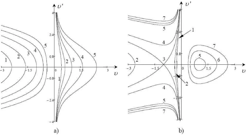
Figure 14. a) Phase plane corresponding to the potential function withC1= 1 and various values ofE.
Line 1: E = −2; lines 2: E = −1; lines 3: E = 0; lines 4: E = 1; lines 5: E = 2. All trajectories in the left half-plane correspond to unbounded solutions. b) Phase plane corresponding to the potential function with C1 =−1 and various values of E. Line 1: E =−4; lines 2: E =−3; lines 3: E =−2;
lines 4: E=−1; lines 5: E= 2.1; lines 6: E= 2.5; lines 7: E= 3.
closed and corresponding solutions are bounded and periodical; they can be expressed in terms of elliptic functions. The phase portrait of such motions is shown in the right half of the phase plane in Fig.14b.
4b. If C1 = 0, but C2 6= 0, the potential function also represents a set of antisymmetric
hyperbolas located either in the third quadrant and right half-plane in Fig. 15 whenC2 = 1, or
in the first quadrant and left half-plane of that figure whenC2 =−1.
Figure 15. Potential function for the case p+q 6= 0, C1 = 0 and two values of C2: C2 = 1 (solid
lines), andC2=−1 (dashed lines). Dotsa,b,canddillustrate possible motion of a point particle in the potential field.
Figure 16. Phase plane corresponding to the potential function (18) withC1= 0. a)C2= 1 and various
values of E. Lines 1: E =−3; lines 2: E =−2; lines 3: E =−1.89; lines 4: E =−1; lines 5: E = 0; lines 6: E = 1; lines 7: E = 2. b) C2 =−1 and various values ofE. Line 1: E =−1; line 2: E = 0; line 3: E = 1; lines 4: E = 2; lines 5: E = 2.5; lines 6: E = 3. All trajectories in the left half-plane correspond to unbounded solutions.
(particle motion to the left from the top of the “hill” corresponds to unbounded solutions). Possi-ble values of particle energyEvary for such motions from minus infinity toPmax= 3(−C2/4)1/3,
wherePmaxis the local maximum of the left branch of the potential function (see Fig.15). The
phase portrait of such motions is shown in the left half-plane in Fig.16a.
Figure 17. Potential function for the casep+q6= 0. a) Supercritical case: C1 =−1 and two values of C2: C2= 1 (solid lines), andC2 =−1 (dashed lines); b) marginal case: C1=−3 and the same two
values of C2; c) subcritical case: C1=−5 and the same two values ofC2 (in the last case the horizontal and vertical scales are doubled).
For the case ofC2 =−1 bounded solutions are smooth periodic waves which correspond to the particle oscillations in the potential well shown in the first quadrant in Fig. 15. Energy is positive for such motion and varies fromPmin= 3(−C2/4)1/3, wherePmin is the local minimum
of the right branch of the potential function (see Fig.15) to infinity. Analytical solution for such waves can be also expressed in terms of cumbersome elliptic functions. Corresponding phase plane is presented in Fig. 16b.
4c. Consider now the case when both C1 6= 0 and C2 6= 0. The shape of the potential
function is more complex in this case in general and depends on the relationship between the constants C1 and C2. The number and values of the potential extrema are determined by the
number of real roots of the equation P′(v) = 0, where prime denotes the derivative on v. This condition yields (see equation (18)):
v3+C1v+ 2C2 = 0.
For real constantsC1 and C2 this equation always has at least one real root. The real root is single when C1≥C1cr≡ −3C
2/3
2 ; its value is given by the expression
v=
q
(C1/3)3+C2 2 −C2
1/3
−(C1/3)
q
(C1/3)3+C2 2 −C2
−1/3 .
Figure 18. Phase plane corresponding to the marginal case,C1=Ccr
1 . a)C1=−3,C2=−1. Line 1: E =−3.05; line 2: E =−3; line 3: E =−2.9; line 4: E =−2; line 5: E = 3.8; line 6: E = 4; line 7:
E = 4.5. All trajectories in the left half-plane correspond to unbounded solutions. b)C1=−3,C2= 1.
Line 1: E=−5; lines 2: E=−4; lines 3: E=−3.75; lines 4: E=−3.5; line 5: E= 2.75; line 6: E= 3; line 7: E= 3.25; line 8: E= 3.5.
local minimum at the right branch of the potential function for C2 =−1 and a local maximum
at the left branch of the potential function for C2 = 1. Almost the same configuration of the
potential function occurs for the marginal case C1 = C1cr, as shown in Fig. 17b, however one more local extremum appears – on the left branch whenC2=−1 and on the right branch when C2 = 1. In the case C1 < C1cr the potential function is shown in Fig.17c; there are three local
extrema of the potential function for any value ofC2 =±1.
The potential configuration in the supercritical caseC1 > C1cr qualitatively is similar to the
case shown in Fig. 15, therefore the corresponding phase portraits are similar to those shown in Fig. 16. In the marginal case,C1 =C1cr, the potential configuration is also similar to those two cases mentioned above, however there are some peculiarities in the phase planes reflecting the appearance of embryos of new equilibrium points. Corresponding phase portraits are shown in Fig. 18. The embryos appear in the vicinity ofE =−3 in Fig.18a and in the vicinity of E= 3 in Fig. 18b.
In the subcritical caseC1 < C1cr the situation is different from the previous ones and should
be considered separately. In the case of C2 =−1, there are two potential wells, one of a finite
depth on the left branch of functionP(v) and another infinitely deep and wide well but bounded from the bottom on the right branch of functionP(v) (see Fig.17c).
For the first potential well there is a family of closed trajectories in the phase plane corre-sponding to periodic solutions with the parameter E varying between the local minimum and maximum of the potential function; these solutions are described by elliptic functions. All closed trajectories are bounded by the loop of separatrix designated by symbol 3 in Fig.19a. Trajecto-ries inside the separatrix loop next to center correspond to quasi-sinusoidal waves, and the loop of the separatrix corresponds to the solitary wave (soliton) which can be treated as the limiting case of periodic waves. The soliton shape is described by the following implicit formula:
η=±√2
v1
2√v2−v1 ln
√
v2−v1+√v2−v
√
v2−v1−√v2−v
+√v2−v
Figure 19. Phase plane corresponding to the subcritical caseC1< C1cr. a)C1=−5,C2=−1. Line 1: E =−6; lines 2: E =−5; line 3: E =−4.25; lines 4: E =−4; line 5: E = 4.7; line 6: E = 5; line 7:
E = 6; line 8: E = 8. All trajectories in the left half-plane outside of the closed loop of separatrix correspond to unbounded solutions. b) C1 =−5, C2 = 1. Line 1: E =−7; line 2: E = −5; lines 3: E=−4.657; lines 4: E=−4; lines 5: E= 4.3; line 6: E= 5; lines 7: E= 6.656; lines 8: E= 7.
Figure 20. Soliton solutions on pedestals as described by equations (19).
wherev1,2=− C1∓
p
C12−3EC2
/E, (v1 < v2) andE=Pmax(C1, C2), wherePmax(C1, C2) is
the value of the potential local maximum shown in the left half-plane of Fig. 17c. Solution (19) is shown in Fig. 20a.
In original variables functionu describing soliton varies in the range
V + 6v1
p+q ≤u≤V +
6v2 p+q;
thus, the soliton amplitude amounts
A= 6v2−v1
p+q =
12
p+q
p
C2
1 −3C2Pmax(C1, C2) Pmax(C1, C2)
; (20)
The soliton velocity is
V =−1
the parameter E varying between the local minimum and maximum of the potential function. All such trajectories are also bounded by the loop of separatrix designated by symbol 7 in Fig.19b. The loop of separatrix corresponds to the solitary wave whose shape is described by the same implicit formula (19), but with different values of constants C1,C2,E and Pmax(C1, C2), wherePmax(C1, C2) is the value of the potential local maximum shown in the right half-plane of
Fig. 17c. This solution is shown in Fig. 20b. All above relationships between soliton amplitude and velocity, as well as between soliton amplitude or velocity and constants C1 and C2 remain
the same as above.
For the infinitely deep well at the origin there are two families of compactons with nonpositive and nonnegative values; the phase plane for them is similar to that shown in Fig.8and solutions are similar to those shown in Fig.9. The entire phase portrait of the system in the case ofC2 = 1
is shown in Fig. 19b. Phase trajectories corresponding to positive compactons are not shown in detail in that figure because they are too close to each other and are in the narrow gap between the axis v′ and external two unclosed branches of the separatix 7 (only one such trajectory, line 5, is shown in Fig. 19b; all other trajectories are similar).
5
Conclusion
As was shown in the paper, the extended reduced Ostrovsky equation (1) possesses periodic and solitary type solutions in general. There is a variety of solitary-wave solutions including compactons with infinite derivatives at the edges, smooth solitons, and periodic waves. All compactons, however, actually are of the compound-type solutions, i.e., they consist of two or more non-smooth branches. Among periodic waves depending on the equation parameters, there are also both smooth solutions and compound-type solutions which consist of periodic sequences of non-smooth branches (see, e.g., Fig. 5b). Moreover, using compacton solutions as the elementary blocks, one can construct very complex compound solutions including stochastic stationary waves.