E l e c t ro n ic
Jo u r n
a l o
f P
r o b
a b i l i t y
Vol. 5 (2000) Paper no. 16, pages 1–28. Journal URL
http://www.math.washington.edu/˜ejpecp/ Paper URL
http://www.math.washington.edu/˜ejpecp/EjpVol5/paper16.abs.html
EIGENVALUE CURVES
OF ASYMMETRIC TRIDIAGONAL RANDOM MATRICES Ilya Ya Goldsheid and Boris A. Khoruzhenko
School of Mathematical Sciences, Queen Mary, University of London, London E1 4NS [email protected],[email protected]
Abstract Random Schr¨odinger operators with imaginary vector potentials are studied in di-mension one. These operators are non-Hermitian and their spectra lie in the complex plane. We consider the eigenvalue problem on finite intervals of lengthnwith periodic boundary conditions and describe the limit eigenvalue distribution whenn→ ∞. We prove that this limit distribu-tion is supported by curves in the complex plane. We also obtain equadistribu-tions for these curves and for the corresponding eigenvalue density in terms of the Lyapunov exponent and the integrated density of states of a “reference” symmetric eigenvalue problem. In contrast to these results, the spectrum of the limit operator in l2(Z) is a two dimensional set which is not approximated by the spectra of the finite-interval operators.
Keywordsrandom matrix, Schr¨odinger operator, Lyapunov exponent, eigenvalue distribution, complex eigenvalue.
1
Introduction
Consider an infinite asymmetric tridiagonal matrixJ with real entries qk on the main diagonal and positive entries pk and rk on the sub- and super-diagonal. Cut a square block of size
n= 2m+ 1 with the center at (0,0) out ofJn and impose the periodic boundary conditions in this block. The obtained matrix has the following form
Jn=
We show nonzero entries of Jn only.
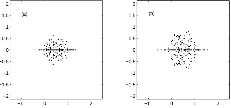
When n is large, the spectrum of Jn cannot be obtained analytically, except for some special choices ofpk,qk, andrk. However, it can be easily computed for “reasonable” values ofnusing any of the existing linear algebra software packages. If thepk, qk, andrk are chosen randomly the results of such computations are striking. For large values of n, the spectra of Jn lie on smooth curves which change little from sample to sample. This was observed by Hatano and Nelson [9, 10]. (b) the sub-diagonal and diagonal entries are drawn from Uni[0,1] and super-diagonal entries are drawn from Uni[12,112].
Fig. 1 shows spectra of two matrices Jn of dimension n = 201. One matrix has its non-zero entries drawn from Uni[0,1]1. Its spectrum is shown on plot (a). Note that this matrix is
1Uni[
only stochastically symmetric. For a typical sample from Uni[0,1], Jn 6= JnT. Nevertheless its spectrum is real. The other matrix has its diagonal and sub-diagonal entries drawn from Uni[0,1] and super-diagonal entries drawn from Uni[12,112]. Its spectrum is shown on plot (b).
Fig. 1 is in a sharp contrast to our next figure. We took the two matrices of Fig. 1 and subtracted
1
2 from all their sub- and super-diagonal entries, including the corner ones. Fig. 1 shows spectra
of the obtained matrices. Note that these spectra have a two-dimensional distribution. As will soon become clear, the eigenvalue curves in Fig. 1 are due to the sub- and super-diagonal entries having the same sign.
−1 0 1 2
−2 −1.5 −1 −0.5 0 0.5 1 1.5 2
(a)
−1 0 1 2
−2 −1.5 −1 −0.5 0 0.5 1 1.5 2
(b)
Figure 2: Spectra ofJn(n= 201) where (a) the sub- and super-diagonal entries are drawn from Uni[−12,12] and the diagonal entries are drawn from Uni[0,1]; and (b) the sub-diagonal entries are drawn from Uni[−12,12], and the diagonal and super-diagonal are drawn from Uni[0,1]
The class of random matrices (1.1) was introduced by Hatano and Nelson in 1996 [9, 10]. Being motivated by statistical physics of magnetic flux lines and guided by the relevant physical setup, they considered random non-Hermitian Schr¨odinger operators H(g) = (id
dx +ig)2 +V and their discrete analogues Jn in a large box with periodic boundary conditions and discovered an interesting localization – delocalization transition. Hatano and Nelson also argued that the eigenvalues corresponding to the localized states are real and those corresponding to the delocalized states are non-real. Since then there has been considerable interest to the spectra of
Jn and their multi-dimensional versions in the physics literature.
as in Fig. 1(a), to a distribution in the complex plane, as in Fig. 1(b), when parameter values of the probability laws of the matrix entries vary.
Our results resemble those obtained in the 1960’s for truncated asymmetric Toeplitz matrices [20, 11]. The eigenvalues of finite blocks of an infinite Toeplitz matrix are distributed along curves in the complex plane in the limit when the block size goes to infinity, see [24] for a survey. Of course, this resemblance is only formal. The class of matrices we consider is very different from Toeplitz matrices.
It is interesting that the spectra of the finite matrices Jn with random entries, even in the limit n → ∞, are entirely different from the spectrum of the corresponding infinite random matrix J = tridiag(pj, qj, rj) considered as an operator acting on l2(Z). Indeed, suppose that the non-zero entries of J are independently drawn from a three-dimensional distribution with a bounded supportS. Then, the probability is one that for any given (p, q, r) ∈S ⊂ R
3 and for
any n∈ N and ε >0 we can always find in J a block of size n such that for all j within this block|pj −p|< ε,|qj −q|< ε, and |rj −r|< ε. By the Weyl criterion, this implies that with probability one the spectrum ofJ = tridiag(pj, qj, rj) contains the spectra of tridiag(p, q, r) for all (p, q, r) ∈S. (This argument is well known in the spectral theory of random operators, see e.g. [5, 18].) Since for every (p, q, r) the spectrum of tridiag(p, q, r) is the ellipse
{z:z=peit+q+r−it, t∈[0,2π]},
the spectrum of the infinite tridiagonal random matrix J has a two-dimensional support with probability one if S is suffiently rich. That is why the eigenvalue curves of Jn are surprising. This discrepancy between the spectra ofJnand J was mentioned in the preliminary account of our work [16] and was one of our motivations for studying the eigenvalue distribution for Jn. Nothing of this kind happens for periodic sequences {(pj, qj, rj)}. If {pk}, {qk} and {rk} have a common period, then the spectrum ofJ lies on a curve in the complex plane [17] coinciding with the eigenvalue curves of Jn in the limit n→ ∞. The two-dimensional spectra are specific to “sufficiently rich” random non-selfadjoint operators (see recent works [7, 8] which contain a much more detailed analysis of the spectral properties of infinite tridiagonal random matrices). One significant consequence of the above mentioned discrepancy between the spectra ofJn and
J is that the norm of the resolvent (Jn−zIn)−1 may tend to infinity as n → ∞ even when z is separated from the spectra of Jn. This aspect of instability inherent in non-normal matrices [21, 23] was thoroughly examined for asymmetric Toeplitz matrices in [19] and for random bidiagonal matrices in [22]. We do not discuss it here.
2
Main results and corollaries
To simplify the notation, we label entries of Jn by (j, k) withj and k being integers between 1 and n. We also setpk=−eξk−1 andrk=−eηk, so thatJn takes the form
Jn=
q1 −eη1 −eξ0
−eξ1 . .. . ..
. .. . .. −eηn−1
−eηn −eξn−1 qn
, (2.1)
where only the non-zero entries of Jn are shown2. The corresponding eigenvalue equation can be written as the second-order difference equation
−eξk−1ψ
k−1−eηkψk+1+qkψk=zψk, 1≤k≤n, (2.2) with the boundary conditions (b.c.)
ψ0 =ψnand ψn+1=ψ1. (2.3)
Our basic assumptions are:–
{(ξk, ηk, qk)}∞k=0 is a stationary ergodic (with respect to translations k−→k+ 1)
sequence of 3-component random vectors defined on a common probability space (Ω,F, P);
(2.4)
Eln(1 +|q0|), Eξ0, Eη0 are finite. (2.5)
The symbol E stands for the integration with respect to the probability measure, Ef =R Ωf dP.
We have chosen the off-diagonal entries ofJn to be of the same sign. More generally, one could consider matrices whose off-diagonal entries satisfy the following condition:
(*) the product of (k, k+ 1) and (k+ 1, k) entries is positive for all k= 1,2, . . . n−1.
Any real asymmetric purely tridiagonal matrix satisfying (*) can be transformed into a sym-metric tridiagonal matrix. The recipe is well known: putψk=wkϕkin (2.2) and choose the wk so that to make the resulting difference equation symmetric. This is always possible when (*) holds, and the weightswk are defined uniquely up to a multiple.
The above transformation is the starting point of our analysis. We setw0 = 1 and
wk=e
1 2
Pk−1
j=0(ξj−ηj), k≥1. (2.6)
Eqs. (2.2)–(2.3) are then transformed into
−ck−1ϕk−1−ckϕk+1+qkϕk=zϕk, 1≤k≤n, (2.7)
ϕn+1= w1 wn+1
ϕ1, ϕn= 1
wn
ϕ0, (2.8)
2
where conditions (2.8). One can visualize this asymmetry: obviously,
W−1JnW =Hn+Vn, (2.10)
Hn is a real symmetric Jacobi matrix. Its eigenvalue equation is given by Eq. (2.7) with the Dirichlet b.c.
ψn+1=ψ0 = 0. (2.13)
Vn, which is due to (2.8), is a real asymmetric matrix. If E(ξ0 −η0) 6= 0 then one of the
two non-zero entries of Vn increases, and the other decreases exponentially fast with n (with probability 1).
Though one could deal directly with Jn, we deal with Hn +Vn instead. We thus consider the asymmetric eigenvalue problem (2.7) – (2.8) as an exponentially large “perturbation” of the symmetric problem (2.7), (2.13). This point of view allows us to use the whole bulk of information about the symmetric problem (2.7), (2.13) in the context of the asymmetric problem (2.7)-(2.8). It is worth mentioning that the exponential rate of growth of Vn is very essential: no interesting effects would be observed for sub-exponential rates.
Following the standard transfer-matrix approach, we rewrite (2.7) as
In order to formulate our results, we need to recall the classical notion of the Lyapunov exponent associated with Eq. (2.7):
It is well known that the limit in (2.16) exists for everyz∈C and is non-negative. Obviously any matrix norm can be used in (2.16), as they all are equivalent. It is convenient for our purposes to use the following norm
||M||= max k
X
j
Introduce
g= 1
2E(η0−ξ0) (2.18)
and consider the curve
L={z∈C : γ¯(z) =|g| }. (2.19) This curve separates the two domains
D1={z∈C : γ¯(z)>|g| } and D2 ={z∈C : γ¯(z)<|g| } (2.20) in the complex plane. Note thatD2 may be empty for some values ofg. In this case,Lis either
empty as well or degenerates into a subset ofR. In Section 3 we prove the following
Theorem 2.1 Assume (2.4) – (2.5). Then for P-almost all ω ={(ξj, ηj, qj)}∞j=0 the following
two statements hold:
(a) For every compact setK1 ⊂D1\R there exists an integer number n1(K1, ω) such that for
alln > n1(K1, ω) there are no eigenvalues of Jn in K1.
(b) For any compact set K2 ⊂D2 there exists an integer number n2(K2, ω) such that for all n > n2(K2, ω) there are no eigenvalues of Jn in K2.
To proceed, we need to introduce another well studied function, the integrated density of states
N(λ) associated with Eq. (2.7). Let
Nn(λ) = 1
n#{eigenvalues ofHn in (−∞;λ)}.
Then
N(λ) = lim
n→∞Nn(λ). (2.21)
It is well known that under assumptions (2.4) – (2.5), the limit in Eq. (2.21) exists on a set of full probability measure and thatN(λ) is a non-random continuous function, see e.g. [5, 18]. It is a fact from spectral theory of random operators that ¯γ(z) and N(λ) are related via the Thouless formula [5, 18]
¯
γ(z) =
Z +∞
−∞
log|z−λ|dN(λ)− Elogc0. (2.22)
According to this formula, ¯γ(z), up to the additive constant E logc0 = 12E(ξ0 +η0), is the
log-potential ofdN(λ):
Φ(z) =
Z +∞
−∞
log|z−λ|dN(λ). (2.23)
Then Lis an equipotential line:
This equipotential line consists typically of closed contoursLj. In turn, each contour consists of two symmetric arcs whose endpoints lie on the real axis. The arcs are symmetric with respect to the reflectionz7→z. The domain D2 defined above is simply the interior of the contours Lj.
Part (b) of Theorem 2.1 states that for almost all {(ξj, ηj, qj)}∞j=0 the spectrum of Jn is wiped out from the interior of every contourLj asn→ ∞. Parts (a) and (b) together imply that for
P-almost all {(ξj, ηj, qj)}j∞=0 the eigenvalues ofJn in the limit n→ ∞ are located on L ∪R. Our next result describes the limiting eigenvalue distribution on L ∪R. Let dν
Jn denote the measure in the complex plane assigning the mass 1/n to each of the neigenvalues ofJn.
Theorem 2.2 Assume (2.4) – (2.5). Then for P-almost all ω ={(ξj, ηj, qj)}∞j=0 the following
statement holds: For every bounded continuous functionf(z) lim
n→∞
Z
C
f(z)dνJn(z) =
Z Σ
f(λ)dN(λ) +
Z
L
f(z(l))ρ(z(l))dl, (2.25)
where
Σ ={λ∈R : λ∈SuppdN, Φ(λ+i0)>max(Eξ0,Eη0) }, (2.26)
ρ(z) = 1 2π
Z +∞
−∞
dN(λ)
λ−z
, z /∈R, (2.27)
and dl is the arc-length element on L.
This theorem is proved in Section 4. Of course the eigenvalue curve L and the density of eigenvalues ρ(z) on it can be found explicitly only in exceptional cases3. However, one can infer from our theorems rather detailed general information about the spectra ofJn in the limit
n→ ∞.
To facilitate the discussion, let us replace our basic assumption (2.4) by the following more restrictive but still quite general one:
{(qk, ξk, ηk)}∞k=0 is a sequence of independent identically distributed random
vectors defined on a common probability space. (2.28)
Under assumptions (2.4) and (2.28), the Lyapunov exponent ¯γ(z) is continuous inz everywhere in the complex plane, see e.g. [2]. Also, there exist positive constants C0 and x0 depending on
the distribution of (ξj, ηj, qj) such that for all |x|> x0
log|x| −C0 <γ¯(x)<log|x|+C0. (2.29)
These inequalities are obvious if the law F of distribution of (ξj, ηj, qj) has bounded support. If the support of F is unbounded, then (2.29) can be obtained using methods of [14, 15]. The continuity of ¯γ(z) together with (2.29) imply that:
(a) Lis not empty if and only if minx∈R¯γ(x)≤ |g|;
(b) Lis confined to a finite disk of radius R depending on the distribution of (ξj, ηj, qj).
3One such case [16, 3] is when
To describe L we notice that ¯γ(x+iy) is a strictly monotone function of y ≥ 0. This follows from the Thouless formula (2.22). Hence, if ¯γ(x+iy) =|g|then
¯
γ(x)≤ |g| (2.30)
and, vice versa, for each x satisfying (2.30) one can find only one non-negative y(x) such that
z=x+iy(x) solves the equation
¯
γ(z) =|g|. (2.31)
Because of the continuity of ¯γ(x), the set ofx where (2.30) holds is a union of disjoint intervals [aj, a′j] with aj < a′j. Therefore L is a union of disconnected contours Lj. Each Lj consists of two smooth arcs,yj(x) and−yj(x), formed by the solutions of Eq. (2.31) whenxis running over [aj, a′j]. Apart from the specified contours, the set of solutions of Eq. (2.31) may also contain real points. These are the points where ¯γ(x) =|g|.
It is easy to construct examples with a prescribed finite number of contours. However we do not know any obvious reason for the number of contours to be finite for an arbitrary distribution of (ξj, ηj, qj).
According to (2.25), the limiting eigenvalue distribution may have two components. One, rep-resented by the first term on the right-hand side in (2.25), is supported on the real axis. We call this component real. The other, represented by the second term, is supported by L. We call this component complex.
The following statements are simple corollaries of our Theorems. Assume (2.4) and (2.28) and considerstochastically symmetric matricesJn, i.e. Eξj = Eηj. In this caseg= 0 and hence the curve L is empty. Therefore the limiting eigenvalue distribution has the real component only. This is surprising and does not seem to be obvious a priori. But even more surprising is thatL remains empty for all
|g|< g(1)cr ≡min
x∈R ¯
γ(x).
If the distribution of (ξj, ηj, qj) is such that the support of the marginal distribution ofqjcontains at least two different points then ¯γ(x) is strictly positive for all x∈ R [5, 18]. In this case, by the continuity of ¯γ(x) and (2.29),gcr(1) >0.
On the other hand, if
|g|> g(2)cr ≡ max
x∈SuppdN¯γ(x).
then Σ of (2.26) is empty and the limiting eigenvalue distribution has the complex component only. Obviously, if the law of distribution of (ξj, ηj, qj) has unbounded support, thengcr(2)= +∞.
Ifg(1)cr <|g|< g
(2)
cr , then the real and complex components coexist.
3
Eigenvalue curves
In this section we prove Theorem 2.1. According to (2.10) the eigenvalues of Jn and Hn+Vn coincide. It is more convenient for us to deal with Hn+Vn and we thus consider the eigenvalue problem (2.7)–(2.8). By (2.14) – (2.15), we may write (ϕk+1, ϕk)T = Sk(z)(ϕ1, ϕ0)T, k =
On the other hand, as required by (2.8),
Therefore the eigenvalue problem (2.7) – (2.8) is equivalent to the following one:
Without loss of generality we may suppose that g≥0. Then, by the ergodic theorem, lim
We start with part (b) of Theorem 2.1. LetK be an arbitrary compact subset ofD2. We shall prove that forP-almost allωthere is an integern0(K, ω) such that for alln > n0(K, ω) equation
(3.6) cannot be solved ifz∈K.
Note thatr(BnSn(z))≤ ||BnSn(z)|| ≤ ||Bn||||Sn(z)||. Therefore, 1
nlogr(BnSn(z)) ≤
1
nlog||Bn||+
1
nlog||Sn(z)|| (3.7)
= o(1) + 1
nlog||Sn(z)||, for almost all ω. (3.8)
Note that we only have to consider the case wheng >0. For, if g= 0 then D2 =∅ and we have
nothing to prove. Obviously, one can findε >0 such that sup
z∈K ¯
γ(z)≤g−ε.
But then, by Theorem A.4 in Appendix, we have, forP-almost all ω, lim sup
n→∞
sup z∈K
1
nlog||Sn(z)||
≤sup z∈K ¯
γ(z)≤g−ε
and hence, by (3.7) – (3.8), lim sup
n→∞
sup z∈K
1
nlogr(BnSn(z))
≤g−ε.
Thus, forP-almost all ω, there exists an integern1(K, ω) such that for alln > n1(K, ω)
1
nlogr(BnSn(z))≤g− ε
2 for all z∈K. (3.9)
Relations (3.9) and (3.3) contradict equation (3.6). This proves part (b) of Theorem 2.1. Now we shall prove part (a) of Theorem 2.1. For this we need the following general (determin-istic) result.
Lemma 3.1 Let q1, . . . , qn be real and c0, . . . , cn be positive. For any two complex numbers φ0
and φ1 define recursively a sequence of complex numbers φ2, . . . , φn+1 as follows:
ckφk+1 = (qk−z)φk−ck−1φk−1, k = 1,2, . . . , n. (3.10)
Denote by Sn the 2×2 matrix which maps (φ1, φ0)T into (φn+1, φn)T obtained as prescribed
above, i.e.Sn(z) =An·. . .·A1, whereAk is given by (2.14). Then for everyz∈C+ the matrix
Sn has two linearly independent eigenvectors (u∗,1)T and (v∗,1)T such that
Imu∗ ≤ −Imz
cn
, |u∗| ≤ |qn−z|
cn
+ c
2
n−1 cnImz
(3.11)
and
Imv∗≥0, |v∗| ≤ c0
Proof. Defineu1, . . . , un+1 as follows: u1 =u and uk+1 =fk(uk),k= 1, . . . n, where
Since Imz and allck are positive, each of the functions fk maps C− into itself and
Imfn(u)≤ −
Therefore,Fn maps continuously the compact setQdefined by the inequalities (3.11) into itself. By the fixed point theorem, there exists u∗ inQ such thatu∗ =Fn(u∗), i.e. ifun+1 =u∗ given
To construct the other eigenvector one can iterate recursion (3.10) in the opposite direction. Namely, set ϕn+1 = vn+1, ϕn = 1 and use (3.10) backwards to obtain the remaining ϕk. continuous in the closure of the upper half of the complex plane and maps this set into itself. Since
|f1˜(u)| ≤ c0
Imz ∀u∈C+, ˜
Fn maps the compact set ˜Q defined by the inequalities in (3.12) into itself. By the fixed point theorem, there exists v∗ ∈Q˜ such that ˜Fn(v∗) = v∗, i.e. ϕ
Lemma 3.2 Let Sn(z) be as in Lemma 3.1 and Bn= diag(βn,1) with βn>0. Then for every
z ∈ C+ the matrix BnSn has two linearly independent eigenvectors (un,1)
T and (v
n,1)T such
that
Imun≤ −
βnImz
cn
, |un| ≤ βn|qn−z|
cn
+βnc
2
n−1 cnImz
(3.15)
and
Imvn≥0, |vn| ≤
c0
Imz (3.16)
Proof. BnSn(z) = ˜An·An−1·. . .·A1, whereA1, . . . , An−1 as before (see (2.14) – (2.15)) and
˜
An=
(qn−z)βn cn −
cn−1βn
cn
1 0
!
Since βn>0, Lemma 3.1 applies.
We now return to our eigenvalue problem (2.7) – (2.8) and to the matrices Sn(z) and Bn associated with this problem, i.e. nowck are given by (2.9) andβn by (3.2). Set
Tn =
un vn
1 1
(3.17)
where (un,1)T and (vn,1)T are the eigenvectors of BnSn(z) obtained in Lemma 3.2.
Lemma 3.3 Assume (2.4) – (2.5). Then for P-almost all {ξk, ηk, qk}∞k=0 the following
state-ment holds: For all z∈C+
lim n→∞
1
nlog||Tn||||T
−1
n ||= 0. (3.18)
The convergence in (3.18) is uniform in z on every compact set inC+.
Proof. For any stationary ergodic sequence of random variables Xn with finite first moment limn→∞Xn/n= 0 with probability 1. By (2.17),
0≤ 1
nlog||Tn||||T
−1
n || ≤ 1
nlog
(|un|+|vn|+ 2)2 |un−vn|
.
To complete the proof, apply inequalities (3.15) – (3.16).
Recall that r(BnSn(z)) is used to denote the spectral radius (3.5).
Lemma 3.4 Assume (2.4) – (2.5). Then for P-almost all {ξk, ηk, qk}∞k=0 the following
state-ment holds: For all z∈C+
lim n→∞
1
nlogr(BnSn(z)) = ¯γ(z), (3.19)
Proof. It follows from Lemma 3.2 thatBnSn(z) = TnΛnTn−1, where Λn is the diagonal matrix of eigenvalues of BnSn(z) corresponding toTn. Then
1 ||Tn||||Tn−1||
≤ ||BnSn||
||Λn|| ≤ ||Tn||||T −1
n ||.
With our choice (2.17) of the matrix norm,||Λ||=r(BnSn(z)) and, by Lemma 3.3, forP-almost all {ξk, ηk, qk}∞k=0,
lim n→∞
1
nlog
||BnSn(z)||
r(BnSn(z))
= 0 uniformly inz on compact subsets of C+. On the other hand, for P-almost all {ξk, ηk, qk}∞k=0,
lim n→∞
1
nlog
||BnSn(z)||
||Sn(z)|| = 0 uniformly in z. This follows from the obvious inequalities
||Sn(z)|| ||B−n1||
≤ ||BnSn(z)|| ≤ ||Bn||||Sn(z)||.
Now the statement of Lemma follows from Theorem A.3 of Appendix. With Lemma 3.4 in hand, we are a in a position to prove part (a) of Theorem 2.1. LetK be a compact subset of D1\R. As ¯γ(z) is continuous inK and ¯γ(z)> g there, one can find an ε >0 such that
min
z∈K¯γ(z)≥g+ε.
From this, by Lemma 3.4, for almost all ω = {ξk, ηk, qk}∞k=0, there exists an integer n1(K, ω)
such that for alln > n1(K, ω)
1
nlogr(BnSn(z))≥g+ ε
2 ∀z∈K. (3.20)
In view of (3.3), (3.20) contradicts (3.6). Theorem 2.1 is proved.
4
Distribution of eigenvalues
We need to introduce more notations and to recall few elementary facts from potential theory. LetMnbe an n×nmatrix. We denote bydνMn the measure onC that assigns to each of then eigenvalues ofMn the mass 1n. This measure describes the distribution of eigenvalues of Mn in the complex plane in the following sense. For any rectangle K⊂C
ν(K;Mn) =
Z
K
dνMn
The measuredνMn can be obtained from the characteristic polynomial ofMn as follows. Let
p(z;Mn) = 1
nlog|det(Mn−zIn)| (4.1)
=
Z
C
log|z−ζ|dνMn(ζ) (4.2) In view of (4.2), p(z;Mn) is the potential of the eigenvalue distribution of Mn. Obviously,
p(z;Mn) is locally integrable in z. Then for any sufficiently smooth functionf(z) with compact support
Z
C
log|z−ζ|∆f(z)d2z = lim ε↓0
Z
|z−ζ|≥ε
log|z−ζ|∆f(z)d2z
= 2πf(ζ),
by Green’s formula. Hence 1 2π
Z
C
p(z;Mn)∆f(z)d2z=
Z
C
f(z)dνMn(z). (4.3) Here ∆ is the two-dimensional Laplacian andd2z is the element of area in the complex plane.
Both p(z;Mn) and dνMn define distributions in the sense of the theory of distributions and Eq. (4.3) can be also read as the equalitydνMn(z) = 21π∆p(z;Mn) where now ∆ is the distributional Laplacian. More generally, it is proved in potential theory that, under appropriate conditions ondν,dν(z) = 21π∆p(z), wherep(z) =R
log|z−ζ|dνMn(ζ) is the potential ofdν. This Poisson’s equation relates measures and their potentials.
In this section we shall calculate the limit ofdνJn for matrices (2.1), obtaining the potential of the limiting measure in terms of the integrated density of statesN(λ) (see (2.21)). Our calculation makes use of relation (2.10) according to which the asymmetric matrixJnis, modulo a similarity transformation, a rank 2 perturbation of the symmetric matrix Hn (see (2.11)). The low rank of the perturbation allows to obtain explicit formulas describing the change in location of the eigenvalues. In our case,
det(Jn−zIn) = det(Hn+Vn−zIn) =d(z;Hn, Vn) det(Hn−zIn), (4.4) were
d(z;Hn, Vn) = det[In+Vn(Hn−zIn)−1] (4.5) = (1 +anGn1)(1 +bnG1n)−anbnG11Gnn (4.6) with an and bn being the top-right and left-bottom corner entries of Vn and Glm standing for the (l, m) entry of (Hn−zIn)−1.
One can easily obtain (4.6) from (4.5) with the help of a little trick. Write Vn in the form
Vn=ATB, where Aand B are the following 2×n matrices:
A=
an 0 . . . 0 0 0 0 . . . 0 1
B =
0 0 . . . 0 1
bn 0 . . . 0 0
.
Then the n×n determinant in (4.5) reduces to a 2×2 determinant, as det[In+ATB(Hn−
Eqs. (4.4) – (4.6) yield the following relationship between the potentials ofdνJn and dνHn:
p(z;Jn) = p(z;Hn+Vn) = p(z;Hn) + 1
nlog|d(z;Hn, Vn)|. (4.7)
The measuresdνHn are all supported on the real axis where they converge to the measuredN(λ) whenn→ ∞. This implies the convergence of their potentials to Φ(z) =R
R
log|z−λ|dN(λ) for all non-real z, see Theorem A.2 in Appendix. Φ(z) is the potential of the limiting distribution of eigenvalues for Hn. Thus the main part of our calculation of p(z;Hn) in the limit n → ∞ is evaluating the contribution of n1 log|d(z;Hn, Vn)| to p(z;Jn). We can do this for all non-real z lying off the curve L (see (2.19) and (2.24)). The corresponding result is central to our considerations and we state it as Theorem 4.1 below. Note that, by the Thouless formula (2.22), ¯
γ(z) =|g|is equivalent to Φ(z) = max(Eξ0,Eη0) and thus (cf. (2.20))
D1={z: Φ(z)>max(Eξ0,Eη0)} and D2 ={z: Φ(z)<max(Eξ0,Eη0) }. (4.8)
Theorem 4.1 Assume (2.4)–(2.5). Then for P-almost all{ξj, ηj, qj}∞j=0,
lim
n→∞p(z;Jn) = Φ(z) ∀z∈D1\
R; (4.9)
lim
n→∞p(z;Jn) = max(Eξ0,Eη0) ∀z∈D2\
R. (4.10)
The convergence in (4.9) – (4.10) is uniform in z on every compact set in D1\R and D2\R
respectively.
Proof. In view of Eq. (4.7) and Theorem A.2 in Appendix, we only have to prove that, with probability one, for any compact setsK1 ⊂D1\R and K2 ⊂D2\R
lim n→∞
1
nlog|d(z;Hn, Vn)|= 0 (uniformly inz∈K1⊂D1\R), (4.11) lim
n→∞ 1
nlog|d(z;Hn, Vn)|= max(Eξ0,Eη0)−Φ(z) (uniformly in z∈K2⊂D2\R). (4.12) Let us writed(z;Hn, Vn) in the form
d(z;Hn, Vn) =anGn1+bnG1n+anbnGn1G1n+ (1−anbnG11Gnn) (4.13) and estimate the four terms on the right-hand side (r.h.s.) of (4.13). Recall thatan andbn are the corner entries ofVn and theG’s are the corner entries of (Hn−zIn)−1. In particular,
G1n=Gn1 =
Qn−1
j=1cj det(Hn−zIn)
= e
1 2
Pn−1
j=1(ξj+ηj)
det(Hn−zIn)
.
Under assumptions (2.4) – (2.5), on a set of full probability measure,
an=−en[
1
2E(ξ0−η0)+o(1)], bn=−e−n[ 1
when n→ ∞ and
e12
Pn−1
j=1(ξj+ηj)=en[ 1
2E(ξ0+η0)+o(1)].
On the other hand,
|det(Hn−zIn)|=enp(z;Hn)=en[Φ(z)−r(z;Hn)],
where r(z;Hn) = p(z;Hn)−Φ(z). According to Theorem A.2 in Appendix for P-almost all {ξj, ηj, qj}∞j=0
lim
n→∞r(z;Hn) = 0 (uniformly in zon every compact set K ⊂
C\R). (4.15) Therefore, with probability one,
|anGn1|=en[Eξ0−Φ(z)+oz(1)] and |bnG1n|=en[Eη0−Φ(z)+oz(1)], (4.16)
where theoz(1) terms vanish when n→ ∞ uniformly inz on every compact set K ⊂C\R. To estimate the third term in the r.h.s. of (4.13), recall the Thouless formula (2.22). As the Lyapunov exponent ¯γ(z) is non-negative everywhere in the complex plane and Φ(z), for every fixed Rez, is an increasing function of|Imz|, we have that
Φ(z)> 1
2E(ξ0+η0) ∀z∈C\R. (4.17) Moreover, since Φ(z) is continuous inz off the real axis,
M(K) := min
z∈K[Φ(z)− 1
2E(ξ0+η0)]>0 for any compact setK ⊂C\R. From this and (4.16),
|anbnG1nGn1| = en[E(ξ0+η0)−2Φ(z)+oz(1)] (4.18)
≤ e−n[2M(K)+oz(1)] ∀z∈K. (4.19) In other words, the third term on the r.h.s. in (4.13) vanishes exponentially fast (and uniformly inz on every compact set inC\R) in the limitn→ ∞.
The fourth term in (4.13) cannot grow exponentially fast withn. Nor it can vanish exponentially fast. Estimating it from above is simple. Since |Gjj| ≤ |Im1z|, j = 1, n, and anbn = eo(n), we have, forP-almost all {ξj, ηj, qj}∞j=0, that
|1−anbnG11Gnn| ≤1 + eo(n)
|Imz|2 ∀z∈C\R (4.20) with theo(n) term being independent of z.
Estimating |1−anbnG11Gnn| from below is less trivial. We do this with the help of the two Propositions stated below. The first one is elementary and the second one is a standard result from spectral theory of random operators [5].
Proposition 4.2 Let Cα={z∈C : α≤argz≤α+π }, where 0≤α≤π. Then min
Proposition 4.3 Under assumptions (2.4) – (2.5), there exists a setΩ0 ⊂Ωof full probability
Remark. For almost all realizations ω, the semi-infinite matrix
11, as a function of z, maps the upper (lower) half of the complex plane
into itself, and so doesGnn. Therefore,
0< α(z;Hn)< π ∀z∈C\R
The r.h.s. in (4.22) is positive and continuous inz∈K. Therefore it is bounded away from zero uniformly in z ∈ K. Hence, for every ω ∈ Ω0 (set of full probability measure) and for every
compact setK ⊂C\R lim inf
where the constantC(K;ω) depends only onK and ω.
Now we are in a position to prove (4.11) and (4.12). Letz∈K ⊂D1\R. Then Φ(z)> Eξ0 and Φ(z)> Eη0 ∀z∈K.
Therefore, by (4.16), the first three terms on the r.h.s. in (4.13) vanish exponentially fast (and uniformly in z∈K) in the limitn→ ∞. But then, with probability one,
lim sup n→∞
1
nlog|d(z;Hn, Vn)| ≤0 (uniformly in z∈K),
in view of (4.20), and lim inf
n→∞ 1
nlog|d(z;Hn, Vn)| ≥0 (uniformly inz∈K),
in view of (4.23). This proves (4.11).
LetK be any compact set inD2\R. Then, by the definition ofD2 and (4.17), min(Eξ0,Eη0)<Φ(z)<max(Eξ0,Eη0).
At this point we may assume, without loss of generality, that Eξ0 6= Eη0. For, if Eξ0 = Eη0
thenD2\R is empty. This follows from (4.17).
Now, if Eξ0 > Eη0 then Eη0 <Φ(z) < Eξ0 for allz ∈ K and, by (4.16), (4.18) – (4.20), the
first term on the r.h.s. in (4.13) dominates the other terms. In this case, with probability one, lim
n→∞ 1
nlog|d(z;Hn, Vn)|= Eξ0−Φ(z) (uniformly in z∈K).
Similarly, if Eξ0 < Eη0, then it is the second term that dominates and, with probability one,
lim n→∞
1
nlog|d(z;Hn, Vn)|= Eη0−Φ(z) (uniformly in z∈K).
Theorem 4.1 is proved.
We shall now deduce from Theorem 4.1 the weak convergence of the eigenvalue distributions
dνJn to a limiting measure in the limit n → ∞. In doing this we shall follow Widom [25, 24] who proved that the almost everywhere convergence of the potentials p(z;Mn) (4.2) of atomic measures dνMn implies the weak convergence of the measures themselves provided they are supported inside a bounded domain in the complex plane. Under assumptions (2.4) – (2.5), the spectra of Jn (2.1) are not necessarily confined to a bounded domain. To extend Widom’s argument to our case we estimate the contribution of the tails of dνJn to the corresponding potentials.
Define
p(z) = max[Φ(z),Eξ0,Eη0]. (4.24)
Φ(z) is a subharmonic function [6] and so is p(z). For, the maximum of two subharmonic functions is subharmonic too. Therefore, ∆p(z) is non-negative in the sense of distribution theory and 21π∆p(z) defines a measure in C which we denote bydν,
dν(z) = 1
2π∆p(z). (4.25)
First, we prove that in the limit n→ ∞ the potentials p(z;Jn) converge to p(z), for P-almost all {ξk, ηk, qk}∞k=0, in the sense of distribution theory.
In the Lemma below C0(C) is the space of continuous on C functions with compact support, andC0∞(C) is the subspace ofC0(C) of those functions which are infinitely differentiable in Rez and Imz.
Lemma 4.4 Assume (2.4) – (2.5). Then on a set of full probability measure, for every f ∈
C0(C), and in particular for every f ∈C It follows from this that on the same set Ω0
lim for every continuousf(z) with compact support and for everyδ >0.
Since f(z) has compact support, f(z)p(z)∈L1(C). Therefore, inn. More precisely, it will suffice to prove the following statement. On a set of full probability measure, for every continuous functionf with compact support
∀ε >0 ∃δ >0 : lim sup n→∞
Z
Lδ
|f(z)p(z;Jn)|d2z < ε. (4.29) Obviously, (4.27) together with (4.28) – (4.29) imply (4.26).
wherez1, . . . , zn are the eigenvalues ofJn and the summation in the two sums in (4.31) is over all eigenvalues ofJnsatisfying the inequalities|zj| ≤Rand|zj|> Rrespectively. The first term in (4.31) is bounded from above but is unbounded from below due to the log-singularities at
zj. On the contrary, the second term is bounded from below, provided z is separated from the boundary of the disk|z| ≤R, but may be unbounded from above due to large values of|zj−z|. We shall treat these two terms separately.
The required estimate on the integral in (4.29) involving the first term in the break-up ofp(z;Jn) (4.31) can be obtained using the property of local integrability of log|z|. Recall that a family of functions{hα(z)}α∈A is called uniformly integrable inz on a bounded setD⊂C if for every
ε >0 there exists a δ >0 such that for every compact set S⊂D of area less thanδ Z
S
|hα(z)|d2z < ε ∀α∈ A.
It is a corollary of the local integrability of log|z|that for every compact setK ⊂C the family of functions {log|ζ −z|}ζ∈K is uniformly integrable in z on bounded subsets of C. From this one immediately obtains
Proposition 4.5 Let χR(|ζ|) be the characteristic function of the disk |ζ| ≤ R. For every compact set K⊂C and for every R >0 the family of functions
n1 n
n
X
j=1
χR(|ζj|) log|ζj−z|
o
n≥1, ζ1,...,ζn∈K
is uniformly integrable in z on bounded subsets of C.
It is now apparent that for every continuousf with compact support and for everyR >0
∀ε >0 ∃δ >0 : lim sup n→∞
Z
Lδ
f(z)1
n X
|zj|≤R
log|zj −z|
d2z < ε. (4.32)
To obtain an appropriate upper bound on the second term in (4.31), note the following. Ifζ is such that dist(ζ,specJn)≥1 then log|z−ζ| ≥0 for every z∈specJn and
0≤ X
|zj|>R
log|zj−ζ| ≤ log|det(Jn−ζIn)| (4.33)
≤ n
X
j=1
log eξj−1 +eηj+|qj|+|ζ|. (4.34)
The latter inequality is due to the fact that for every matrix A = ||Ajk||n
j,k=1, |detA| ≤ Qn
j=1 Pn
k=1|Ajk|.
By Theorem 2.1, all non-real eigenvalues of Jn are in the vicinity ofL for all sufficiently large
only once there. Therefore the probability is one that, moving up along the imaginary axis say,
By the ergodic theorem, under assumptions (2.4) – (2.5), on a set Ω1of full probability measure,
lim
(4.32) and (4.35) imply (4.29). Lemma 4.4 is proved.
Corollary 4.6 Assume (2.4) – (2.5). Then with probability one,
lim
n→∞dνJn =dν
in the sense of weak convergence of measures.
Proof. Since the operation ∆ is continuous on distributions, Lemma 4.4 implies that, on a set of full probability measure,
dνJn(z) = 1
2π∆p(z;Jn)→
1
as distributions. To complete the proof, recall that a sequence of measures converging as
distri-butions must be converging weakly [12].
It is apparent that ∆p(z) = 0 everywhere off a line consisting of two parts. One is the equipo-tential lineL (2.24) that separates the domainsD1 andD2; the other is Σ (2.26) which is made up of all points of SuppdN that do not belong to the interior of the closed contours ofL.
p(z) is continuous in the upper and lower parts of the complex plane. It also has continuous derivatives everywhere but on L and Σ. Its normal derivative has a jump whenz moves from
D2 to D1 in the direction perpendicular to L. It follows from this that the restriction dνC of
dν to C\R is supported on Land has there density ρ(z) with respect to the arc-length measure
dl on L. The density equals the jump in the normal derivative of p(z) multiplied by 21π. A
On the other hand, the restriction dνR of dν to the real axis is supported on Σ and coincides there withdN. Therefore, for every bounded continuous function f(z)
Z Taking into account that the weak convergence of measuresdνn is equivalent to the convergence of R
f(z)dνn(z) on bounded continuous functions we obtain from (4.36) – (4.37) and Corollary 4.6 the statement of Theorem 2.2.
A
Appendix
In our analysis of the non-self-adjoint eigenvalue problem (2.7)-(2.8) we have used a number of results about the finite difference equation
−ck−1ϕk−1−ckϕk+1+qkϕk=zϕk (A.1) with random coefficientsck and qk. For the sake of completeness, we reproduce here the corre-sponding formal statements. With the exception of Theorem A.4 these results are well known in the theory of random selfadjoint operators. Their proofs together with references to the original publications can be found in books [5, 18]. Some of the results are proved there under slightly less general assumptions than those used in this paper. However only minor adjustments are needed to extend the published proofs to the generality of our assumptions.
Given a sequence of 2-component vectors{(ck, qk)}∞j=1, consider a sequence of tridiagonal
Assume that
ω ≡ {(cj, qj)}∞j=1 is a stationary ergodic (with respect to the translation k→k+ 1)
sequence of random vectors defined on a common probability space (Ω,F, P); (A.2)
ck>0 for all k, and Eln(1 +|q1|)<+∞, E|lnc1|<+∞. (A.3)
Here as before the symbol E denotes averaging ever the probability space.
The matrixHn is symmetric and has real eigenvalues. Their empirical cumulative distribution function is defined as
Nn(λ, ω) = 1
n#{eigenvalues ofHn in (−∞, λ)}.
Theorem A.1 Assume (A.2) – (A.3). Then there exists a continuous non-random function
N(λ) of real variable λsuch that for almost all sequences ω
lim
n→∞Nn(λ, ω) =N(λ).
In other words, on a set of full probability measure, the eigenvalue counting measures dNn(λ, ω)
converge weakly, asn→ ∞, to the limiting measure dN(λ).
The limit distribution function, N(λ), is called the integrated density of states (IDS) of Eq. (A.1).
Let
p(z, Hn) =
Z +∞
−∞
log|λ−z|dNn(λ, ω) (A.4) and
Φ(z) =
Z +∞
−∞
log|λ−z|dN(λ). (A.5)
Under assumptions (A.2) – (A.3), the integral in (A.5) converges for every non-real z, hence Φ(z) is well defined off the real axis. On the real axis, the equality in (A.5) is understood in the following sense4
Φ(x) = lim ε↓0
Z +∞
−∞
max[log|λ−x|,−ε−1]dN(λ), x∈R
with the convention that Φ(x) =−∞ if the above limit is −∞5. With this convection, Φ(z) is subharmonic in the complex plane. In particular, Φ(z) is upper semi-continuous.
Theorem A.2 Assume (A.2) – (A.3). Then the following is true for almost all ω: For all non-real z
lim
n→∞p(z;Hn) = Φ(z). (A.6)
The convergence in (A.6) is uniform in z on every compact subset of C\R.
4
Under assumptions (A.2) – (A.3), the prelimit integral converges for everyε >0
5In fact, Φ(
Let
γn(z, ω) = 1
nlog||Sn(z)||, (A.7)
whereSn(z) is as in (2.15).
The Lyapunov exponent is defined as follows: ¯
γ(z) = lim
n→∞Eγn(z, ω).
The limit above exists for every z ∈C. Any matrix norm can be used in (A.7), as they all are equivalent. Since ||Sn||2 ≥ |detSn|and detSn(z) =c
0/cn, we have that for everyz∈C, and in particular for every real z,
¯
γ(z)≥0.
Theorem A.3 Assume (A.2) – (A.3). Then for almost all ω the following is true: For every compact set K⊂C\R
lim
n→∞γn(z, ω) = ¯γ(z) uniformly in z∈K.
Remark. In contrast to non-realz, on the real axis lim
n→∞γn(x, ω) =γ(x, ω), (A.8)
The limit above exists for almost all pairs (x, ω) and Eγ(x, ω) = ¯γ(z). However, whenxis fixed, the set Ωx of thoseω for which the limit in (A.7) exists depends onx, andP(∩x∈ΣΩx) = 0 (see
[14, 15, 1]).
For everyω,γn(z, ω) is a subharmonic function in the complex plane. ¯γ(z) is also subharmonic inC. This property of the Lyapunov exponent is very useful, see [6]. We use it here to deduce the following corollary from Theorem A.3.
Theorem A.4 Assume (A.2) – (A.3). Then for almost all ω the following is true: For every compact set K⊂C, and in particular for every compact set K ⊂R,
lim sup n→∞
sup z∈K
γn(z, ω)
≤sup z∈K ¯
γ(z).
If, in addition, γ¯(z) is continuous in K then
lim sup n→∞
sup z∈K
[γn(z, ω)−γ¯(z)]
Remark. This theorem plays a crucial role in our proof of the fact that the eigenvalues ofJnare wiped out, asn→ ∞, from the interior of each contour of the curveL, see part (b) of Theorem 2.1. Actually, our proof of part (a) of Theorem 2.1 also applies to any compact subset ofD2\R. However, this proof is based on Theorem A.3 and cannot be applied to the whole interior of L as it contains intervals of real axis.
Theorem A.4 follows immediately from Theorem A.3 and the following result from the theory of subharmonic functions:
Theorem A.5 [see [13], p. 150] Let uj ≡/ − ∞ be a sequence of subharmonic functions in C
converging in the sense of distribution theory to the subharmonic functionu. If K is a compact subset of C and f is continuous on K, then
lim sup j→∞
sup K
(uj−f)
≤sup K
(u−f).
Theorem A.6 (Thouless formula) For all z∈C, γ¯(z) = Φ(z)− Elogc1.
It is a corollary of the Thouless formula and the positivity of the Lyapunov exponent ¯γ(z) that
Φ(z)≥ Elogc0 ∀z∈C. (A.9)
References
[1] Avron, J. and Simon, B. (1983), Almost Periodic Schr¨odinger Operators II., Duke Math. Journ. 50, 369 – 391.
[2] Bougerol, P. and Lacroix, J. (1995), Products of Random Matrices with Applications to Random Schr¨odinger Operators. Birkh¨auser, Boston.
[3] Brezin, E. and Zee, A. (1998), Non-Hermitian localization: Multiple scattering and bounds.
Nucl. Phys. B509[FS], 599 – 614.
[4] Brouwer P. W., Silvestrov, P. G., and Beenakker, C. W. J. (1997), Theory of directed localization in one dimension.Phys. Rev. B56, R4333 – R4336.
[5] Carmona, R. and Lacroix, J. (1990), Spectral Theory of Random Schr¨odinger Operators.
Birkh¨auser, Boston.
[6] Craig, W. and Simon, B. (1983),Subharmonicity of the Lyapunov Index.Duke Math. Journ. 50 (1983), 551 – 560.
[8] Davies, E. B., Spectral theory of pseudo-ergodic operators. To appear in Commun. Math. Phys.
[9] Hatano N. and Nelson, D. R. (1996), Localization transitions in non-Hermitian quantum mechanics. Phys. Rev. Lett. 77, 570 – 573.
[10] Hatano N. and Nelson D. R. (1997),Vortex pinning and non-Hermitian quantum mechanics.
Phys. Rev.B56, 8651 – 8673.
[11] Hirshman Jr., I. I. (1967), The spectra of certain Toeplitz matrices. Illinois J. Math. 11, 145 – 159.
[12] H¨ormander, L. (1983),The analysis of linear partial differential equations, Vol. I.Springer, New York.
[13] H¨ormander, L. (1994)Notions of Convexity.Birkh¨auser, Boston.
[14] Goldsheid, I. Ya. (1975),Asymptotic behaviour of a product of random matrices that depend on a parameter. Dokl. Akad. Nauk. SSSR224, 1248 – 1251.
[15] Goldsheid, I. Ya. (1980),Asymptotic properties of the product of random matrices depending on a parameter. In Adv. in Prob. 8, pp. 239 – 283, Ya. G. Sinai and R. Dobrushin, eds. Dekker, New York.
[16] Goldsheid I. Ya. and Khoruzhenko, B. A. Distribution of eigenvalues in non-Hermitian Anderson models.Phys. Rev. Lett. 80, 2897 – 2900 (1998).
[17] Naiman P. B. (1964),On the spectral theory of non-symmetric periodic Jacobi matrices (in Russian). Zap. Meh.-Mat. Fak. Har’ kov. Gos. Univ. i Har’kov. Mat. Obsc., (4), 30, 138 – 151.
[18] Pastur, L. A. and Figotin, A. L. (1992),Spectra of Random and Almost-Periodic Operators.
Springer, Berlin.
[19] Reichel, L. and Trefethen, L. N. (1992), Eigenvalues and pseudo-eigenvalues of Toeplitz matrices. Lin. Alg. Appl. 162-4, 153 – 185.
[20] Schmidt, P. and Spitzer, F. (1960), The Toeplitz matrices of an arbitrary Laurent polyno-mial. Math. Scand.8, 15 – 38.
[21] Trefethen, L. N. (1991) Pseudospectra of matrices. In D. F. Numerical Analysis 1991, pp. 336 – 360, Griffiths and G. A. Watson, eds. Longman Scientific and Technical, Harlow, Essex, UK, 1992.
[22] Trefethen, L. N. Contendini, M., and Embree, M., Spectra, pseudospectra, and localization for random bidiagonal matrices. To appear in Commun. Pure and Appl. Math.
[23] Trefethen, L. N., Trefethen, A. E., Reddy, S. C., and Driscoll, T. A. (1993),Hydrodynamic stability without eigenvalues.Science 261, 578 – 584.
![Figure 1: Spectra of Jn (n = 201) where (a) all non-zero entries are drawn from Uni[0, 1]; and(b) the sub-diagonal and diagonal entries are drawn from Uni[0, 1] and super-diagonal entriesare drawn from Uni[12, 112].](https://thumb-ap.123doks.com/thumbv2/123dok/969963.913511/2.612.106.493.423.608/figure-spectra-entries-diagonal-diagonal-entries-diagonal-entriesare.webp)