Policy Analysis in a General
Equilibrium Framework
Shujie Yao, University of Portsmouth, UK Aying Liu, University of Middlesex, UK
In a developing economy where agriculture has an important role in economic growth and in maintaining a certain level of living standards for the poor, any macro-economic and sectoral policies have critical implications on income distribution and government finances. This article develops a computable general equilibrium (CGE) model to describe a multiregional, multimarket, and multiagent agrarian economy. The model is initially aimed for the Philippines, but can be extended to any other country in southeast Asia. A number of policies regarding supply, demand, and external trade are simulated to compare their costs and benefits, paying particular attention to poverty alleviation, income distribution, price stability, economic growth, and government finances. 2000 Society for Policy Modeling. Published by Elsevier Science Inc.
1. INTRODUCTION
In a developing country where agriculture has an important role in economic growth and the well-being of the poor, any policy reform has important implications on income distribution, price stability, and government finances. This article constructs a com-putable general equilibrium (CGE) model that can incorporate alternative government policies directed towards achieving a cer-tain set of economic and social objectives, paying particular atten-tion to agricultural producatten-tion, income distribuatten-tion, government budget, and external balance of payments.
Address correspondence to Shujie Yao, Department of Economics, University of Ports-mouth, Portsmouth PO4 8JF, UK.
The authors are grateful to the comments made by two anonymous referees and the editor, but they remain solely responsible for any remaining omissions or errors.
Shujie Yao is professor and director of development economics research; Aying Liu is lecturer.
Received February 1997; final draft accepted September 1997.
Journal of Policy Modeling22(5):589–610 (2000)
Most CGE studies have focused on the two ends of the commod-ity chain, i.e., the producers (farm-gate or factory-gate) and the final consumers, ignoring the marketing segment between produc-tion and final consumpproduc-tion (see Robinson, 1986, for a survey; Clarete and Roumasset, 1986 and 1987, for the Philippines; Naray-ana et al., 1991, for India; and Zhuang, 1994, for China; Schul, 1974, Adelman and Robinson, 1986, and Kilkenny, 1993, for the United States). Moreover, many studies have treated the entire economy as one single homogeneous market without paying atten-tion to geographical differences. The importance of geographical diversity has been recognized by many authors (Kilkenny, 1993, Roberts and Russell 1994) but few authors have attempted to incorporate the intermediate market segment between producers and consumers into their studies. To overcome the limitations of previous studies, this paper constructs a general equilibrium model with three distinctive characteristics: (1) it concentrates specifically on the food system by treating nonfood agriculture, nonagricul-tural sector, and the rest of the world as other aggregate sectors of the economy; (2) it separates the country into two regions with different farming systems and incomes; and (3) it divides the economy into three different market levels: farm-gate, wholesales, and retail. The present model is based on the Philippines economy in 1987, but it can be extended to any other countries in southeast Asia such as Thailand, Malaysia, or Indonesia.
In most countries, governments enter the market with specific objectives, policy instruments, and acting agents. In the food sec-tor, the main acting agent for the government is the National Food Authority (NFA), which can enter any of the three market-ing levels. Many price and marketmarket-ing policies can be implemented through NFA’s buying and selling activities. All the policy objec-tives require special instruments that can be incorporated into the CGE framework. In this paper, although our focus is on the structure of the model, four sets of policy changes are simulated to examine their effects on the nutritional status of the poor, price stability, income distribution, economic growth, and government finances. The costs and benefits of each policy scenario are ana-lyzed to show how policy reforms should best be implemented in an empirical sense.
POLICY ANALYSIS IN A GE FRAMEWORK 591
2. THE ECONOMIC SITUATION IN THE PHILIPPINES
Although most countries in southeast Asia are among the fastest growing economies in the world over the last 3 decades, the Philip-pines has been left behind by its ASEAN (Association of South-east Asian Nations) neighboring states, especially Malaysia and Thailand, since the 1980s (Table 1; Balisacan, 1992). In the 1970s, the growth rate of per capita domestic gross product, GDP, in the Philippines was very close to those in Indonesia, Thailand, and Malaysia. Political instability and poor economic management in the early 1980s resulted in an overall contraction of the economy by more than 1 percent per year. Although the economy recovered quite strongly in the late 1980s, the average growth rate of per capita GDP was only 1 percent per year from 1980–90, compared with 5.2 to 7.6 percent in the other three countries. Although economic reform and trade liberalization had some positive results in the early 1990s, economic growth was still slow. The average annual growth rate of per capita GDP was only 1.6 percent from 1990–94, compared with 8.4 percent in Malaysia, 8.2 percent in Thailand, and 7.6 percent in Indonesia.
Widespread poverty, heavy debts, and high unemployment rate have been persistent characteristics of the postwar Philippines economy. The size of total external debts reached US$39.3 billion in 1994, imposing a considerable burden to the economy. The debt servicing requirements are now a serious handicap to successful development policies.
For a long period of time, excessive taxation on agricultural production has led to massive transfers of resources from agricul-ture to the industrial sector. Industry has nevertheless been unable to compete in the world market and unable to absorb surplus labor from agriculture. These factors reflect the nature of the country’s economic policies, which tend to favor urban consumers and industrial producers at the expense of agriculture and rural producers. The tariff structure has consistently favored the manu-facturing sector. Agriculture, on the another hand, received nega-tive protection (5% in 1985). The overvaluation of the peso through most of the postwar period was a major disincentive to agricultural production and exports, which was one of the main reasons for accumulating trade deficits and external debts (McCar-thy, 1990; Guzman, 1987).
S.
Yao
and
A.
Liu
Table 1: Population and Economic Indicators of ASEAN-4, 1970–79
Period Indonesia Philippines Thailand Malaysia
A. Population (million) 1994 190.0 67.0 58.0 20.0
Average annual growth (%) 1970–80 2.4 2.5 1.7 2.4
1980–90 1.8 2.4 1.8 2.6
1990–94 1.6 2.2 1.0 2.4
B. GNP/head (US$) 1991 610.0 730.0 1570.0 2520.0
1994 880.0 950.0 2410.0 3480.0
Average annual growth (%) 1985–94 6.0 1.7 8.6 5.6
C. Average annual GDP Growth (%) 1970–80 7.2 6.0 7.1 7.9
1980–90 6.1 1.0 7.6 5.2
1990–94 7.6 1.6 8.2 8.4
D. Average annual agricultural growth (%) 1970–80 4.1 4.0 4.4 n.a.
1980–90 3.4 1.0 4.0 3.8
1990–94 3.0 1.6 3.1 2.8
E. Total external debts ($bil.) 1980 20.9 17.4 9.3 6.6
1994 96.5 39.3 61.0 24.8
As % of total exports 1980 94.7 233.9 104.5 46.8
1994 211.3 189.7 107.9 39.0
As % of GNP 1980 28.0 53.7 25.9 28.0
1994 57.4 59.7 43.1 36.9
POLICY ANALYSIS IN A GE FRAMEWORK 593
the foreseeable future. Two thirds of the country’s labor force is employed in agriculture or activities linked to agriculture. Eco-nomic development will not have a stable base until there is enough food to meet the domestic demand.
The current administration has been trying to stimulate eco-nomic growth through raising agricultural production. It also has many other objectives, such as raising the income of farm families, improving the balance of payments situation, and protecting the poor during the process of structural adjustment.
To achieve these goals, the government faces a number of policy conflicts. The first conflict is between the need to stimulate agricul-tural growth and the need to hasten industrial development (Net-tleton, 1992). The second conflict is between the need to improve food self-sufficiency and the need to increase agricultural exports. Given land and other resource constraints, encouraging agricul-tural exports by whatever means will depress food security, or vice versa. During the 1970s and the early 1980s, exports were taxed while food production was subsidized. In recent years, there has been a tendency to shift production from food to export crops. As a result, the food deficit has increased, especially in rice.
3. THE CGE MODEL
A computable general equilibrium (CGE) model based on a social accounting matrix (SAM) is the natural tool to assess policy impacts on the economy. A CGE model provides a framework in which government policies can be assessed as to how they will impact on different aspects of the economy, including food production, food consumption, income distribution, government finances, market prices, and internal and external debts.
3A. The Food System in the Philippines
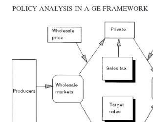
The country is divided into two regions, north and south. Rice is produced in both regions. Sugar is produced by the estate farms in the north, and maize by small farms in the south. Government enters the production system by imposing a floor price paid to rice farmers through NFA and taxing agricultural inputs.
The marketing subsystem determines how much of each com-modity is sold and through which channel. As a main staple food, rice is marketed both by private traders and NFA. The other commodities are solely marketed by private agents.
There are two stages in the distribution system. In the first stage, rice changes hands from producers to private traders or NFA. The market share of each will depend on the ratio between the floor price offered by NFA and the market price. NFA buys at the prevailing market price unless this drops below the floor price, in which case it will buy at the floor price. The wholesale market price is endogenously determined by market clearing between supply and demand at the farm-gate.
In the second stage, rice changes hands from the traders (NFA or private traders) to final consumers through the retail market. The market share of each will depend on the ratio between the ceiling price charged by NFA and the market price. NFA sells at the prevailing market price unless this rises above the ceiling price, in which case it will sell at the ceiling price. The retail market price is determined by market clearing supply and demand at the retail market. NFA has a monopoly on rice imports and holds a carry-over stock, which may be maintained at a minimum level as a security stock. The marketing and distribution of other com-modities is entirely conducted by the private sector. There are no floor or ceiling prices.
Government intervention in the marketing subsystem may in-volve the following methods: floor and ceiling prices for rice, target rice sales by NFA, rice imports, security stock, sales tax on private traders, and import and export tariffs. Figure 1 demonstrates the complete commodity chain from production to consumption of agricultural products, incorporating external trade, stock, govern-ment intervention in the marketing of rice, and in taxation at different market levels.
POLICY ANALYSIS IN A GE FRAMEWORK 595
Figure 1. Commodity chain and government intervention in agriculture.
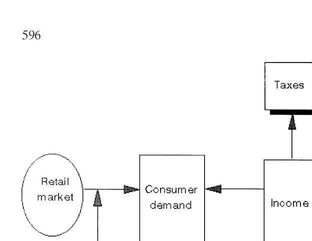
is also regarded as a consumer who “consumes” all the other commodities except rice, sugar, and maize. Thus, there are nine distinctive consumer groups.
Consumers have income from four different sources: land reve-nue, labor, profits, and income support from the government. Consumer demand is determined by income and prices. Govern-ment intervenes in the consumption system through the following means: income tax, income support to the poor, and ceiling price for rice (Figure 2). The income support mechanism is govern-ment’s deliberate policy to alleviate poverty and to improve in-come distribution.
Figure 2. The consumption system and income support mechanism.
other consumer groups, government has its own income and ex-penditure pattern.
3B. The Social Accounting Matrix (SAM)
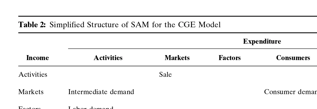
According to the food system presented in 3A, a SAM is con-structed to show the major revenue and expenditure transactions among production activities, markets, factors of production, con-sumption, and exogenous accounts (i.e., Government Stock, and the Rest of the World). The SAM is a 54354 matrix. A simplified matrix is shown schematically in Table 2.
Like other conventional SAMs, the SAM in Table 2 contains the blocks of activities, factors, consumers, government, stocks, and the rest of the world (ROW). The only difference is that it contains a separate block of markets. Therefore, the products of activities flow into markets instead of final consumers. Farm-gate prices are formulated at the entrance of markets whereas retail prices are formulated at the exit.
POLICY
ANALYSIS
IN
A
GE
F
RAMEWORK
597
Table 2: Simplified Structure of SAM for the CGE Model
Expenditure
Income Activities Markets Factors Consumers Government Stock ROW
Activities Sale Production Clearing
subsidies stock
Markets Intermediate demand Consumer demand Government Commodity
demand exports
Factors Labor demand Factor
exports
Consumers revenue from investment Labor income Income Transfers
or profit support
Government Indirect taxes, Factor income Income taxes Loan/aid
Investment revenue,
Stock Opening stock Saving Saving
ROW Investment revenue Commodity Factors Transfers Debt service
imports imports
their activities. Producers have to buy materials from the markets, pay to labor, consumers as factor owners, the government as a tax collector and factor owner, and ROW in column 1. The opening stock is carried over from the previous period. In row 2, the markets have to meet the demands of intermediate inputs, con-sumers, the government, and exports. To satisfy these demands, the markets absorb sales from activities and imports from abroad in column 2. In row 3, factors receive income from activities and ROW. Factor income is distributed to consumers, the government and ROW in column 3. Consumers in row 4 receive incomes from activities, labor income from factors, income support from the government, and income transferred from ROW. They buy com-modities from the markets, pay taxes to the government, save in the stock, and sent money abroad in column 4. In row 5, the government receives income from activities, factors, income taxes from consumers, and loans and grants from ROW. It subsidizes production, buys commodities from the markets, provides income support to the poor, saves, and pay debts to ROW in column 5. In row 6, total stock comes from three sources: opening stock, savings from consumers and the government. It is cleared in col-umn 6 under activities. In row 7, ROW receives incomes from activities, markets (material imports), and factors (factor imports), consumers (income transfers out), and debt services. ROW in column 7 injects money into the economy through the markets (exports), factors (exports), consumers (income transfers in), and the government (loans and grants).
The CGE model explicitly represents seven commodities, six primary producers, two intermediate agents, nine consumer groups, and nine factor inputs for production.
3C. Major Equation Systems
The basic model is made up of 250 equations. The variables in the model can be categorized into three groups: (1)policy vari-ables, which represent government intervention in the economy; (2)exogenous variables, which are outside the control of govern-ment such as rainfall and world prices; and (3)outcome or endoge-nous variables, which measure the effects of policy changes.
POLICY ANALYSIS IN A GE FRAMEWORK 599
government), and constant elasticities of substitution (CES) be-tween any pair of competitive prices (or markets). In this section, only the core behavioral equations are listed and described, the entire equation system, including many identities (or accounting) equations are discussed in Greener and Liu, 1993, Appendix B.
All the equations are in the form of proportional changes, repre-sented by the symbold. This means that quantities such as balances that are simple sums when expressed in levels become more com-plex expressions when expressed in proportional changes. The model variables are represented by capital letters. Wherever a variable name appears without adin front of it, it represents the previous year’s value. Model parameters are represented by Greek letters in all equations (e.g.,a,b). Exogenous and policy variables are all underlined in the equations (e.g., ER for the exchange rate). The model contains a total of 37 blocks of equations, each of which may be repeated a number of times to cover the range of the subscripts to which it refers. Subscripts are used to denote the disaggregation of the variables into model accounts as follows: (1) activities,a 51, 2, . . . , 7; (2) market, m5 1, 2; (3) factors,
f 51, 2, . . . , 9; and (4) consumers, c5 1, 2, . . . , 9. The production function, Eq. (1):
dQPa5
o
fWc
fa·dFfa2 ga·dCL, (1)
where QPa is production of activity a; Wcfa is the ratio of factor cost to output value; Ffais factor demand by activity a of factor
f;gais climate elasticity of activitya; CL is climate index. Propor-tional change in production is the sum of the changes in factor demand, weighted by cost shares. The final term simulates the effect of a change in climate.
Sales to markets, Eq. (2):
dSAam5 dQPa1 ssa(dPm2 dPa), (2)
whereSAam is sales by activity a to market m, ssa is elasticity of substitution between markets,Pmis price in marketm,Pais average selling price of activity a. The change in sales is determined by the change in production and a price term governing substitution between markets.
Average selling price, Eq. (3):
dPa5
o
mWs
amdPm, (3)
whereWs
m. This equation calculates the average selling price of a product as the weighted sum of the prices in different markets.
Retail price index, Eq. (4):
dPc5
o
mWd
mcdPm, (4)
whereWd
mcis values share of purchases by consumercfrom market
m. This equation calculates the average buying price of the retail markets.
Average buying price, Eq. (5):
dBPa5
o
mWd
amdPm, (5)
where BPa is the average buying price of activity a, Wdam is the quantity share of purchases by activity a from marketm.
Intermediate demand, Eq. (6):
dIDma5 dQa2 sda(dPm2 dBPa), (6)
whereIDmais intermediate demand by activity a from marketm,
sd
a is elasticity of demand substitution between markets. The change in intermediate demand is given by the change in quantity produced or purchased (assuming all quantity elasticities are equal to 1), and a price term that governs the strength of substitution between markets. This equation applies under the simplifying assumption that all the possible substitutions between markets have the same elasticity. income from activity a,FSfis supply of factorf,Wficfis value share of income from factorf, CSUB is consumer subsidy, and Wsu
c is the value share of subsidy.
Consumer expenditure, Eq. (8):
dEc5
(Yc·dYc2ITXc·dITXc)
Ec
(8)
Consumer expenditure, or disposable income,Ec, is the difference between income and taxation,ITXc.
Consumer demand, Eq. (9):
dCDmc5 bdmc(dEc2 dPm)2 sdc(dPm2 dPc) (9)
where bd
POLICY ANALYSIS IN A GE FRAMEWORK 601
demand substitution between markets. The proportional change in consumer demand is expressed as the sum of an income effect and a price effect.
Government demand, Eq. (10):
dGD5 dGCE2 dPro. (10)
Government demand, GD, is calculated from the exogenously specified government consumption expenditure, GCE, corrected by the endogenous change in price,Pro, in the market from which government demands for “retail others.”
Price margin, Eq. (11):
dMa5
Pa·dPa2BPa·dBPa2Pa· PTXRa· (dPa1 dPTXRa)
Ma
. (11)
This equation calculates the proportional change of the price mar-gin, Ma, for all activities, by subtracting the buying price (BPa) from the selling price (Pa), and subtracting the production tax (calculated by the change in tax rate, PTXRa).
Factor demand, Eq. (12):
dFfa5 soaWoa(dPa2 dPf)1 sia
o
f9Wi
f9a(dPf92 dPf). (12)
The proportional change in factor demand, Ffa, is expressed as the sum of an output effect and a price substitution effect. The output effect is obtained by multiplying the input–output substitu-tion elasticity, soa, by the share of output to profit, Woa, and the difference between the proportional changes in output price and the factor price. The price effect is obtained as the sum over possible factors of the input–output substitution elasticity, sia, multiplied by the share of factor demand to profit, Wifa, and the difference between the proportional changes in price between factors where substitution takes place.
Profit, Eq. (13): wherePais profit of activitya, PSUais production subsidy,PTXa is production tax,Wo
ais share of output value to profit,Wsua is share of subsidy value to profit,Wfd
fais share of factor demand value to profit,Wtx
by the combination of five terms: output value, producer subsidies, factor costs, indirect tax, and value of opening stock.
Government income, Eq. (14):
whereGYdenotes government income, Wp
a value share of profit income, Wfi
f value share of factor income, Wti value share of tax income, GL grants and loans from the rest of the world. ER exchange rate, and Wgl value share of grants and loans income. Government income consists of four terms: profit, factor income, tax income, grants and loans from the rest of the world.
Government expenditure, Eq. (15):
where GE is government expenditure,Wgceis expenditure share of government consumption,Wpsis expenditure share of producer subsidies, DS is debt servicing, Wcs is expenditure share of con-sumer subsidies, Wds is expenditure share of debt servicing, ER is exchange rate, and PSUais subsidy to activitya. The proportional change of total government expenditure is defined as the sum of four exogenous terms: government consumption, producer subsid-ies, consumer subsidsubsid-ies, and debt servicing.
External balance, Eq. (16):
dEB5EX·dEX1GL·dGL2IM·dIM2DS·dDS
EB . (16)
External balance,EB is defined by adding the value of exports,
EX, and external grants and loans,GL, and subtracting the value of imports,IM, and debt servicing payments,DS.
Floor price, Eq. (17):
Pwr(11 dPwr)>FLOORwr. (17)
The price paid by NFA in the wholesale rice market,Pwris greater than or equal to the exogenous floor rice price,FLOORwr.
POLICY ANALYSIS IN A GE FRAMEWORK 603
Prr(12 dPrr)<CEILINGrr. (18)
The price charged by NFA in the retail rice market, Prr is less than or equal to the exogenous ceiling rice price,CEILINGrr.
4. DATA AND POLICY SIMULATIONS
The data required to establish the CGE model consists of two main components. One is the SAM, which formulates the base scenario of the economic system and provides an initial condition for simulation. The other is a set of parameters that determines model behavior.
The SAM is constructed based on 1987 data from the 1991 Philippines Statistical Yearbook (1991). Data from other sources are also used, including the World Development Report (World Bank), World Trade (World Bank), Debt Table (World Bank), and the Asian Development Statistics (Asia Development Bank), and many country studies relevant to the Philippines.
Apart from a large amount of original data, many parameters are also used in the model. These include the supply and demand elasticities for commodities, production elasticities of factors, trade substitute elasticities of commodities, etc. These parameters are sets of coefficients, which are related to technological aspects of the model. Some of them are estimated using traditional statistical inference; some are collected from the existing literature; some have to be guessed, because there is no detailed information avail-able. All parameters, however, have been calibrated to be consis-tent with existing trends over 1987–91.
Before conducting any policy simulations, it is essential to iden-tify the main problems faced by the country. Any policies that have large effects on such problems are deemed to be important and should be closely examined. In the Philippines, the most serious problems are food security for the poor, skewed income distribution, heavy internal and external debts, and unstable eco-nomic growth. The policies identified to have sizeable effects on these problems based on the CGE model can be classified into three groups: supply side policies, demand side policies, and trade policies.
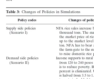
Table 3: Changes of Policies in Simulations
Policy codes Changes of policy and main objectives
Supply side policies NFA rice sales increase by 50 percent from 864 to 1300 (Scenario I) thousand tons. The main objective is to stabilize
the market price of rice. Floor price of rice is raised up to the market level from 4530 to 6198 pesos/ ton. NFA has to bear all the marketing costs from the farm-gate to the market. The main objective is to raise domestic rice production.
Demand side policies Income supports to rural tenants and urban poor double (Scenario II) from 120 to 240 pesos per head. The main objective
is to reduce poverty. Rural income tax rate at 1.5 percent is eliminated. Urban poor income tax rate is halved from 3.5 to 1.75 percent. Urban rich income tax rate is doubled from 8.6 to 17.2 percent. The main objectives are to raise government revenue and to redistribute incomes to the advantage of the poor. The NFA ceiling price of rice sales is reduced by 5 percent from 6510 to 6185 pesos/ton.
Exchange rate policy Devaluation of the peso from 24.2/$ to 27/$. The main (Scenario III) objective is to stimulate agricultural production and
exports.
Demand and exchange rate Combination of Scenarios II and III. policy (Scenario IV)
records the percentage changes over the base-run results except the two rows for government budgetary deficits and balance of payments, which are recorded in level terms under all policy sce-narios.
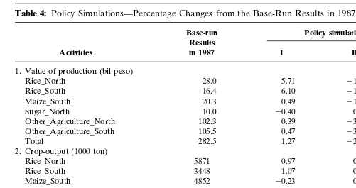
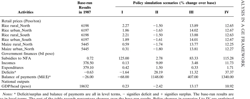
The results in Table 4 can be interpreted as follows. The main objective of scenario I is to encourage rice production by doubling NFA rice sales and by raising the floor price of rice. Increasing rice sales by NFA depresses market prices and farm incomes. Raising the floor price has an opposite effect. Overall, the value of agricultural production rises because of higher prices. Household incomes of all groups decline because the negative price effect is greater than the income effect of increased rice production. Government subsidies to NFA rise by 125 percent, and the budget-ary deficit rises from 0.63 to 1.64 billion pesos. The trade deficit also increases due to a shortfall of sugar production.
POLICY
ANALYSIS
IN
A
GE
F
RAMEWORK
605
Table 4: Policy Simulations—Percentage Changes from the Base-Run Results in 1987
Base-run Policy simulation scenarios (% change over base) Results
Activities in 1987 I II III IV
1. Value of production (bil peso)
Rice_North 28.0 5.71 21.43 13.86 12.50
Rice_South 16.4 6.10 21.22 14.02 12.80
Maize_South 20.3 0.49 21.77 13.79 12.12
Sugar_North 10.0 20.40 0.30 15.00 15.30
Other_Agriculture_North 102.3 0.39 23.13 13.98 11.39
Other_Agriculture_South 105.5 0.47 23.13 14.03 11.41
Total 282.5 1.27 22.65 14.05 11.81
2. Crop-output (1000 ton)
Rice_North 5871 0.97 0.12 20.07 0.07
Rice_South 3448 1.07 0.12 20.06 0.06
Maize_South 4852 20.23 0.06 20.10 20.06
Sugar_North 16991 20.78 20.02 20.26 0.08
3. Income (peso/head)
Landowner_North 13383 20.28 21.23 0.16 20.66
Tenant_North 7600 20.39 0.37 20.16 0.39
Urban rich_North 92211 21.57 21.48 0.70 20.49
Urban poor_North 10357 21.56 20.27 0.56 0.42
Landowner_South 13382 20.60 21.28 0.01 20.87
Tenant_South 7600 20.68 0.41 20.20 0.38
Urban rich_South 92211 21.57 21.47 0.70 20.49
Urban poor_South 10357 21.56 20.27 0.56 0.42
S.
Yao
and
A.
Liu
Table 4: Continued
Base-run Policy simulation scenarios (% change over base) Results
Activities in 1987 I II III IV
4. Rice Consumption (kg/head)
Landowner_North 176.1 21.19 20.11 0.00 0.06
Tenant_North 166.2 21.38 0.42 20.18 0.06
Urban rich_North 156.5 21.28 23.39 22.11 23.32
Urban poor_North 134.8 22.37 0.89 0.22 1.04
Landowner_South 146.7 21.30 20.07 20.07 0.00
Tenant_South 141.8 21.55 0.42 20.28 0.00
Urban rich_South 127.1 21.26 23.30 20.16 23.23
Urban poor_South 111.7 22.33 0.90 0.18 1.07
4A. Maize consumption (kg/head)
Landowner_North 68.0 0.15 20.29 0.00 20.15
Tenant_North 63.0 0.00 0.32 20.16 0.00
Urban rich_North 82.0 20.24 21.46 20.24 21.59
Urban poor_North 63.0 0.16 1.27 0.79 1.27
Landowner_South 98.0 0.00 20.31 0.00 20.10
Tenant_South 93.0 20.11 0.32 20.22 0.00
Urban rich_South 122.0 28.36 29.51 28.36 29.67
Urban poor_South 93.5 20.64 0.43 20.11 0.43
5. Farm-gate prices (pesos/ton)
Rice_North 4769 3.54 21.72 13.92 12.56
Rice_South 4769 3.48 21.72 13.92 12.56
Maize_South 4190 0.72 21.98 13.75 12.12
Maize_North 4190 0.72 21.98 13.75 12.12
POLICY
ANALYSIS
IN
A
GE
F
RAMEWORK
607
Table 4: Continued
Base-run Policy simulation scenarios (% change over base) Results
Activities in 1987 I II III IV
6. Retail prices (Peso/ton)
Rice rural_North 6198 2.27 21.50 13.89 12.65
Rice urban_North 6197 1.86 21.63 14.02 12.67
Rice rural_South 6198 2.21 21.50 13.88 12.63
Rice urban_South 6197 1.89 21.61 14.01 12.67
Maize rural_North 5445 0.59 21.74 13.77 12.25
Maize urban_North 5445 0.31 21.80 13.81 12.27
8. Government finances (bil peso)
Subsidies to NFA 0.72 125.00 2.78 83.33 115.28
Incomes 378.50 0.13 9.09 3.48 11.73
Expenditures 379.10 0.42 1.50 0.33 1.71
Deficits* 20.63 21.64 28.19 11.32 37.37
Balance of payments (Mil.$)* 226.00 268.00 1148.00 407.00 1340.00
9. National outputs
GDP/head (peso) 18632 0.23 22.42 13.17 10.92
groups was more than 10 times that of the poor groups. Eliminating income tax on the poor and raising taxes on the rich could lead to a significant improvement in government finances and income distribution. However, reforming income taxes alone does not help redistribute income from the rich to the poor. It needs to be supported by a direct income support to the targeted groups, rural tenants, and urban poor. The positive effects of such policy reforms are marginal in terms of income distribution, although government finances, and the balance of payments improve significantly. There is a small increase in per capita income of the tenant groups. One major negative effect is that per capita GDP shrinks by 2.42 percent. Agricultural production also declines as a result of depressed market prices.
Currency devaluation in scenario III produces some powerful impacts on the economy. The most obvious positive impact is a substantial improvement on the balance of payments and govern-ment budget, which are critical for the country to reduce its huge internal and external debts. The improvement on GDP, and the increased values of production and personal incomes, however, are largely due to inflated domestic prices rather than real produc-tion as a result of currency devaluaproduc-tion. Combining scenarios II and III produces the most desirable result on income distribution. The low income groups, rural tenants, and urban poor all benefit from this mixture of policies. The negative effects of tax reforms on production are eliminated. The positive effects on government budget and on the balance of payments reinforce each other.
5. CONCLUSIONS
POLICY ANALYSIS IN A GE FRAMEWORK 609
The policy simulation results in Section 4 demonstrate that many kinds of policy changes can be simulated from the CGE framework. In the context of the Philippines, as the most important concerns of the economy are the efficient use of agricultural re-sources, the reduction of huge internal and external debts, and the reduction of poverty and undernourishment of the poor, several alternative policy scenarios are included in the simulations to investigate the impacts of such policies on different important indicators of concern.
REFERENCES
Adelman, I., and Robinson, S. (1986) U.S. Agriculture in a General Equilibrium Frame-work: Analysis with a Social Accounting Matrix.American Journal of Agricultural Economics68:1197–1206.
Asia Development Bank.Asian Development Statistics(various issues).
Balisacan, A.M. (1992) Rural Poverty in the Philippines: Incidence, Determinants and Policies.Asian Development Review1.
Clarete, R., and Roumasset, J. (1987) A Shoven-Whalley Model of a Small-Open Economy: An Illustration with Philippines Tariffs.Journal of Public Economics1.
Clarete, R., and Roumasset, J. (1986)Modelling Agricultural Development Policy: A General Equilibrium Approach. School of Economics Discussion Paper No. 86-7, University of Philippines.
Greener, R., and Liu, A. (1993)Agricultural Policy Analysis in a General Equilibrium Framework: An Introduction to the AGRISM Model for the Philippines. Interna-tional Development Centre discussion paper, University of Oxford.
Guzman, G.G. (1987)Phillipines: General Trends in Agriculture, Agricultural Output and Input Pricing. Tokyo: Asian Production Organization.
Kilkenny, M. (1993) Rural/urban effects of terminating farm subsidies.American Journal of Agricultural Economics75:968–980.
McCarthy, F.D. (1990)Problems of Developing Countries in the 1990s, Vol II. World Bank Discussion Papers, Country Studies.
Narayana, N.S.S., Parikh, K.S., and Srinivasan, T.N. (1991)Agricultural Growth and Distri-bution of Income: Policy Analysis with a General Equilibrium Model of India. Amsterdam: North-Holland.
Nettleton, G. (1992) The Philippines—Land of Promise.Food Matters15.
Organisation of Economic Cooperation and Development (OECD). (1990)Financial & External Debt of Developing Countries, 1990 Survey.
The Philippines Statistical Yearbook. (1991).
Roberts, D., and Russel, N. (1994)Income Distribution and the Structure of Production: Insights from a SAM-based Model of UK Agriculture. Discussion Paper, Department of Agriculture Economics, University of Manchester, UK.
Robinson, S. (1986)Multi-Sectoral Models of Developing Countries: A Survey. Department of Agricultural and Resource Economics, Working Paper, No. 401, University of California, Berkeley.
World Bank, Debt Tables (various issues).
World Bank, World Development Report (various issues). World Bank, World Tables (various issues).