ELECTRONIC COMMUNICATIONS in PROBABILITY
REFLECTED BROWNIAN MOTION IN A WEDGE:
SUM-OF-EXPONENTIAL STATIONARY DENSITIES
A.B. DIEKER1
H. Milton Stewart School of Industrial and Systems Engineering, 765 Ferst Drive NW, Atlanta GA 30332-0205, USA
email: [email protected]
J. MORIARTY2
School of Mathematics, University of Manchester, Oxford Road, Manchester M13 9PL, UK email: [email protected]
SubmittedJanuary 10, 2008, accepted in final formOctober 7, 2008 AMS 2000 Subject classification: 60J65, 60J60, 60K25
Keywords: Reflected Brownian motion with drift – stationary distribution – reflection principle
Abstract
We give necessary and sufficient conditions for the stationary density of semimartingale reflected Brownian motion in a wedge to be written as a finite sum of terms of exponential product form. Relying on geometric ideas reminiscent of the reflection principle, we give an explicit formula for the density in such cases.
1
Introduction
It is well-known that Brownian motion on the positive half-line with negative drift and reflection at zero has a stationary density which is exponential. One derivation of this fact uses time reversal to relate the distribution of the corresponding transitory process at time tin the driftless case to the distribution of the maximum of a standard Brownian motion over[0,t], which can be found using the reflection principle. A Cameron-Martin-Girsanov change of measure then introduces the drift, and letting t→ ∞gives the required stationary distribution. In the d-dimensional setting, analogous arguments show that in certain situations, semimartingale reflected Brownian motion (SRBM) in a polyhedral cone has a stationary density which can be written as a finite sum of terms of exponential product form—that is, terms of the form x7→ae−〈λ,x〉for somea∈R,λ∈Rd. We call such a density asum of exponentials. The aim of this paper is to give necessary and sufficient conditions under which the stationary density of SRBM in a two-dimensional wedge can be written as a sum of exponentials.
1FINANCIALLY SUPPORTED IN PART BY THE SCIENCE FOUNDATION IRELAND, GRANT NUMBER SFI04/RP1/I512,
AND A POSTDOCTORAL FELLOWSHIP FROM THE IBM T.J. WATSON RESEARCH CENTER, YORKTOWN HEIGHTS NY, USA.
2FINANCIALLY SUPPORTED IN PART BY THE SCIENCE FOUNDATION IRELAND, GRANT NUMBER SFI04/RP1/I512.
In order to motivate our study, we describe the above argument in a multidimensional setting in Section 2 below. The invariant measure for SRBM with special pushing directions at the boundary of a polyhedral cone then relates to exit probabilities for the corresponding free Brownian motion. For some cones, in analogy with the one-dimensional case, these exit probabilities can be obtained explicitly using the reflection principle. If the reflected process is positive recurrent, then upon differentiating we obtain a stationary density which can be written as a sum of exponentials. Since the latter can thus be viewed as a natural multidimensional extension of the exponential stationary density of one-dimensional SRBM, this raises the question under what circumstances the stationary distribution of a given SRBM in a polyhedral cone has a sum-of-exponential density. This paper shows that, for SRBM in a two-dimensional polyhedral cone, sum-of-exponential stationary densities arise well beyond those cases to which the above arguments can be applied.
The stationary distribution of multidimensional SRBM in a polyhedral cone is only known in rel-atively few cases. It has a density consisting of a single exponential term under a skew-symmetry condition on the pushing directions on the faces[17, 25]. We also mention an apparently isolated example due to Harrison [13] and work of Foschini [11]; we discuss the latter in more detail below. In the absence of further explicit results, numerical techniques have been developed[6] and logarithmic tail asymptotics have been investigated[3, 9, 14].
Before describing our results in more detail, we introduce some notation which is summarised in Figure 1. Define the wedge as
S={x∈R2: 0≤arg(x)≤ξ}.
Throughout this paper we write wθ = (cosθ, sinθ)forθ ∈R. Given some 0< δ,ε,ξ < π, we setv1=kv1kwδ, v2=kv2kwξ−ε. Let F1andF2 be the two faces of the wedge. As is customary, we normalise v1 and v2 such that 〈v1,n1〉 =1 and 〈v2,n2〉= 1, where n1 and n2 are the unit normal vectors on F1 and F2, respectively. Let some vector µ ∈ R2 also be given, and write
θµ=arg(µ)∈(−π,π]. A key role in this paper is played byα, which is introduced by Varadhan and Williams[22]as
α=δ+ε−π
ξ .
Our results concern the caseα <1, and it is well-known (e.g.,[22, 24]) that under this condition there exists a continuous semimartingale Markov process with properies that can intuitively be summarised as follows (we do not give the mathematically rigorous definition here, as it can be found in, e.g.,[3, 10, 24]). The process behaves like a standard Brownian motion with drift−µin the interior of the wedgeS, at the boundary of the wedge it is pushed in some specified direction, and the time it spends at the vertex of the wedge has Lebesgue measure zero. The pushing directions are constant along each of the faces, and are given byvifor thei-th face. We call this process SRBM in a wedge and seek its stationary distribution, which is absolutely continuous with respect to Lebesgue measure[5, 16].
We prove that the stationary density of this process is a sum of exponentials if and only ifα=
ξ
v1 v2
n1 n2
F1 F2
θµ
ε
δ
−µ
Figure 1: The wedgeS.
arguments suggested by the reflection principle, and consequently obtain an explicit formula for the stationary density. A discrete-state space version of Foschini’s algorithm, the compensation method, has been successfully applied to a variety of queueing problems[1, 2]. Another body of work loosely related to the present paper studies (driftless) two-dimensional SRBM withα=−1 [8, 19], motivated by a connection with Schramm-Loewner evolutions.
This paper is organised as follows. Section 2 gives some background and discusses the special sum-of-exponential stationary densities mentioned above. Section 3 contains our main result and gives a geometric construction of the stationary density. In Sections 4–6, we prove the main result.
2
Survival probabilities, reflection groups, and Weyl chambers
This section describes a special class of sum-of-exponential stationary densities which can be ob-tained directly using time reversal. These densities motivate our main result, since they typify the general structure of a sum-of-exponential stationary density.
Consider an SRBM as in Figure 1, with drift−µandδ=ε=ξ. Suppose thatµ∈So(the interior of S) to ensure positive recurrence, and writeΠfor the stationary measure of the SRBM. Time reversal gives
Π({y∈S:〈y,n1〉 ≤ 〈x,n1〉,〈y,n2〉 ≤ 〈x,n2〉}) =P−x(T =∞), (1) wherePy is the law of the corresponding free Brownian motionB starting in yandT is the first exit time from−S, i.e.,T =inf{t≥0 :B(t)6∈ −S}. To see this, we use the wedge−Sto define a partial order<onR2(see for example[20]) and then if ˜Bs=Bt−s−Bt,
sup{Bs: 0≤s≤t} −Bt < xif and only if (2)
sup{−x+B˜s: 0≤s≤t} < 0, (3)
Biane et al.[4] have recently shown that if the wedge angle is of the formξ=π/mfor some integerm≥2 then
P−x(T=∞) =
X
w∈G
sgn(w)e−〈µ,(I−w)x〉 (4)
for any x ∈So and anyµ∈So, where the sum is taken over the finite reflection groupG with associated signature function sgn(·), as detailed below. We remark that this formula gives the probability that a standard Brownian motion with drift never exits a so-called Weyl chamber—in particular, it is not restricted to a two-dimensional setting.
We next describe the index of summation in (4), i.e., the elements of the reflection group G. Throughout, we represent any element of R2 as a column vector. Write Rθ for the reflection matrix across the line with argumentθ, i.e.,
Rθ=
cos 2θ sin 2θ
sin 2θ −cos 2θ
andρθ for the rotation matrix over an angleθ, i.e.,
ρθ=
cosθ −sinθ
sinθ cosθ
.
The groupGconsists of the 2mmatricesI,Rξ,ρ2ξ,ρ2ξRξ, . . . ,ρ2(m−1)ξ,ρ2(m−1)ξRξ. The signature of the matricesρ2kξRξis−1, while the signature of the others is+1.
On combining (1) and (4), we find that the stationarydensityof SRBM withξ=δ=ε=π/mis
proportional to X
w∈G
sgn(w)〈µ,(I−w)v2〉〈µ,(I−w)v1〉e−〈µ,(I−w)x〉. (5) This is a sum of 2m−3 nonzero terms, since the prefactor vanishes when w= I, w =Rξ, and
w = ρ2(m−1)ξRξ. It is the aim of this paper to put the explicit formula (5) into the context of more general SRBMs. Specifically, we show that every sum-of-exponential stationary density has a representation reminiscent of (5).
3
Main results
This section presents our main result on sum-of-exponential stationary densities, and explains its geometric interpretation. Our result shows that sum-of-exponential stationary densities can be written as determinants with a special structure. The proofs are deferred to Sections 4–6.
The matrices
Rotk=ρ2δ+2kξ and Refk=ρ2δ+2(k−1)ξRξ (6) fork≥0 play an important role in our main theorem. Write
Θℓ={θ∈(ξ−ε,δ): sin(θ−2δ−kξ)6=0 fork=0, . . . , 2ℓ}.
We know from Hobson and Rogers[18]and from Dupuis and Williams [10]that there exists a unique stationary distribution of the SRBM ifξ−ε < θµ < δ. Let pµ be its density with respect to Lebesgue measure, and writee1for the vector(1, 0). For integersj, we also define the function
πµj :S→Rthrough
πµj(x) =〈µ,(I−Rotj)v1〉e
−〈µ,(I−Rotj)x〉− 〈µ,(I−Ref
j)v1〉e−〈µ,(I−Refj)x〉
Observe that bothpµandπµj depend onδ,εandξ, which is suppressed in the notation. Theorem 1. The following are equivalent:
(i) α=−ℓfor some integerℓ≥0;
(ii) α=−ℓfor some integerℓ≥0and for allµwithθµ ∈Θℓ, the functions pµandπµ are equal
up to a multiplicative constant, where for x∈S,
πµ(x) =
In part (ii) of this theorem, the conditionθµ ∈Θℓprevents a certain degeneracy which is funda-mental to the problem. Indeed, it guarantees the linear independence of the exponential functions inπµ. We remark that the determinant in (ii) has a different form than the ones recently studied in connection with transition probabilities for certain Markov chains[7].
A straightforward calculation using Vandermonde matrices shows that the functionπµ defined by (7) may be written as
This representation forπµis used later in the proof of Theorem 1; note that each exponential term is characterised by a rotation or a reflection matrix, Rot0, Ref1, Rot1, . . . , Refℓ, Rotℓ.
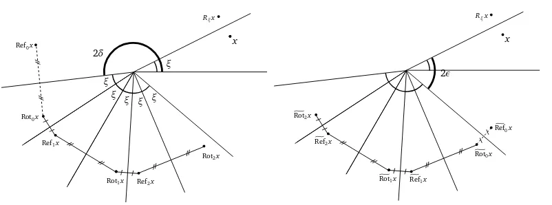
Although there is not necessarily an underlying reflection group in the general setting of Theo-rem 1, the rotation and reflection matrices in TheoTheo-rem 1 suggest a connection with the reflection-group framework. We illustrate this forα=−2 (henceℓ=2) in the leftmost diagram of Figure 2, where we depict the five points Rot0x, Ref1x, Rot1x, Ref2x, Rot2x for an arbitrarily chosen x∈S. By construction, Rot0xlies in the wedgeρ2δS, which we call the ‘initial wedge’. The other points Ref0x, Rot1x, . . . are constructed by successive reflections, reminiscent of the orbit of Rot0xunder the action of a reflection group. In particular
ξ ξ
ξ ξ ξ ξ
x
2δ
Rξx
Ref0x
Rot0x
Ref1x
Rot1x Ref2x
Rot2x
x
2ε
Rξx
g
Rot2x
Ý
Ref2x
g
Rot1x RefÝ1x
g
Rot0x Ý
Ref0x
Figure 2: An anticlockwise construction ofπµ(left) and a clockwise construction of ˜πµ(right).
• Two points lying in adjacent wedges—that is, wedges which share a common boundary line—are reflections of each other in that line.
Note that Ref0x, although not contributing to πµ since (I −Ref0)v1 = 0, is also obtained by reflection from Rot0x. We indicate this by a dashed line in Figure 2.
Ifα=−ℓthen the last point lies in the wedgeρ2δ+2ℓξS, which is the same asρ−2εS. On comparing this with the initial wedgeρ2δS, it transpires that thelastwedge in the anticlockwise construction given above is thefirstwedge in the following clockwise construction. Fork≥0 we introduce the matrices
g
Rotk=ρ−2kξ−2ε and RefÝk=ρ−2(k−1)ξ−2εR0.
The rightmost diagram of Figure 2 illustrates a clockwise construction for the stationary density, starting with the wedge ρ−2εS and labelling the points using the matrices gRotk and RefÝk. The problem is exactly the same as in the leftmost diagram, so by uniqueness the corresponding sum-of-exponential densities must agree onS. We use this observation in the proof of Theorem 1. We close this section by stating some properties of the functionπµ defined in (7), which play an important role in our proof of Theorem 1. These properties are proved in Section 4. We start with a result for the coefficients{ck}defined in (9).
Lemma 1. Let −α = ℓ ∈ {1, 2, . . .} and θµ ∈ Θℓ. The coefficients ck defined by (9) satisfy, for 1≤k≤ℓ,
ck〈µ,(I−Refk)v1〉〈µ,(I−Rotk−1)v2〉=ck−1〈µ,(I−Refk)v2〉〈µ,(I−Rotk−1)v1〉. (10) Using this lemma, it is readily checked that (5) is recovered from Theorem 1 by settingδ=ε=
ξ=π/m. Indeed, we then have〈µ,(I−Rotk−1)v1〉=〈µ,(I−Refk)v1〉, so that (10) reduces to ck〈µ,(I−Rotk−1)v2〉=ck−1〈µ,(I−Refk)v2〉.
In this special case we may therefore set
ck=〈µ,(I−Rotk)v2〉=〈µ,(I−Refk)v2〉, and we obtain (5).
Proposition 1. If−α=ℓ∈ {1, 2, . . .}, then for anyθ ∈[0,ξ]and anyµ withθµ ∈Θℓ, we have
πµ(r w
θ)∼Cµrℓsin(ℓθ+δ)as r→0, where Cµ is a finite nonzero constant independent of r and
θ.
Our next result is that πµ defined by (7) does not change sign on S. Note that this resolves Conjecture 1 in Dai and Harrison[6]for the special class of SRBMs studied in this paper.
Proposition 2. The functionπµ does not change sign on S.
4
Properties of
π
µIn this section, we prove the properties ofπµclaimed in Section 3. The proof of the main result, Theorem 1, is deferred to Sections 5 and 6.
4.1
Proof of Lemma 1
We first divide (10) by sin(θµ−δ−kξ)sin(δ+ (k−1)ξ), which is nonzero as a consequence of the assumption onµin conjunction with the identityδ+ε=π−ℓξ. Again using this identity, we find after some elementary trigonometry that (10) is equivalent to, withωk=θµ−2δ−kξ,
cksin(kξ)sin(ωℓ+k) =−ck−1sin((ℓ+1−k)ξ)sin(ωk−1). To show that this holds for theckdefined in (9), we observe that
〈µ,(Refk−Rotk)v1〉sin(ω2(k−1)) =〈µ,(Refk−1−Rotk−1)v1〉sin(ω2k)
and that
〈µ,(Roti−Rotj)e1〉=−2 sin((j−i)ξ)sin(ωi+j). After some algebra we also find that
sin(kξ)sin(ωℓ+k)sin(ω2(k−1)) Y 0≤i<j≤ℓ;i,j6=k
〈µ,(Roti−Rotj)e1〉
= sin((ℓ−k+1)ξ)sin(ωk−1)sin(ω2k) Y 0≤i<j≤ℓ;i,j6=k−1
〈µ,(Roti−Rotj)e1〉,
and the claim follows.
4.2
Proof of Proposition 1
For simplicity we suppose thatkµk=1. We first investigate the behaviour near zero ofπµ(x), for which we rewrite e〈µ,x〉πµ(x)using the determinantal representation (7). A key ingredient is the identityercos(η)=I0(r) +2
P∞
row as
In conjunction with some trigonometry, the above reasoning shows that
e〈µ,x〉πµj(x) =I0(kxk) + Bessel functions of the first kind, and forn≥1 the coefficient in front ofIn(kxk)is proportional to
¯
To see how this follows from (7), note that we may apply elementary determinantal operations to replace a row with elements cos(ω2j)mbyU
m(cos(ω2j)). The termI0(kxk)is not present in the expansion in view of the last row in (12) with ones.
The conditionθµ∈Θℓguarantees that none of the cos(ω2j)are equal, and we conclude that the coefficient ofIn(kxk)vanishes forn< ℓand that it is proportional to sin(ℓθ+δ)forn=ℓ. Since Iℓ(r)∼C rℓfor some constantC6=0 asr→0, this yieldsπµ(r wθ)∼Cµrℓsin(ℓθ+δ).
4.3
Proof of Proposition 2
Lemma 2. Letℓ∈ {1, 2, . . .}andζ∈Rℓ+1. For any y>0, the sign of the determinant
Proof. The statement is a continuous analogue of the claim thats(n,0,...,0)(ζ)is nonnegative for
ζ≥0, wheresλis a symmetric polynomial known as a Schur polynomial (or, in this special case, a complete homogeneous symmetric polynomial).
By induction onℓone can show that the given determinant equals
Y
We now prove Proposition 2. By the Maximum Principle (see Theorem 2.5 of[21]for a suitable form), neither the minimum nor the maximum ofπµ overS is attained in the open setSo. We therefore investigate the boundary. equality of the signs follows from Proposition 1 after showing that they do not depend on r. From Lemma 2 withζj=〈µ, Rotje1〉and (11) we conclude this forπµ(r w0). Applying the same argument ‘clockwise’ shows that this also holds forπµ(r wξ).
5
The BAR and a PDE with boundary conditions
5.1
The BAR
Our proof of Theorem 1 requires the Basic Adjoint Relationship (BAR) as presented in following proposition, which is implied by Propositions 3 and 4 in[6]; see[5]for proofs.
Proposition 3. Suppose thatα <1and assume the existence and uniqueness of a stationary distri-bution for the SRBM.
A nonzero finite measure ν0 on S is proportional to the stationary distribution if and only if there exist finite measuresν1on F1andν2on F2such that for any f ∈C2
b(S)
Z
S
1
2∆f − 〈µ,∇f〉
dν0+
Z
F1
〈v1,∇f〉dν1+
Z
F2
〈v2,∇f〉dν2=0 (BAR).
Letσandσibe the Lebesgue measures onSandFi, respectively. Writevi∗=2ni−vi. Proposition 4. Let p∈C2(S)be nonnegative and integrable over S.
If (BAR) is satisfied with dν0=p dσand dνi=p/2dσi, then
∆p+2〈µ,∇p〉 = 0 on So, (13) 〈v1∗,∇p〉+2〈µ,n1〉p = 0 on F1o, (14)
〈v2∗,∇p〉+2〈µ,n2〉p = 0 on F2o. (15) Conversely, if (13)–(15) hold and moreover p(0) =0, then (BAR) is satisfied with dν0= p dσand dνi=p/2dσi.
Proof. We may repeat the arguments in the proof of Lemma 7.1 of Harrison and Williams[17]. The additional assumptionp(0) =0 ensures that (7.8) in[17]automatically holds. The above proposition motivates investigating sum-of-exponential solutions to (13)–(15).
5.2
Sum-of-exponential solutions to the PDE
In this subsection we study some properties of sum-of-exponential solutions to the PDE (13) plus either boundary condition (14) or (15). We use the following observation, due to Foschini[11, Sec. III.A].
Lemma 3. Let p be given by p(x) =Pki=1aie−〈ci,x〉for some k<∞, a
i 6=0, and ci 6=0such that
ci6=cjif i6= j.
If p satisfies (13) and (14), then for each i=1, . . . ,k precisely one of the following holds: 1. x7→e−〈ci,x〉satisfies (14), or
2. there exists a unique j 6= i such that x 7→ aie−〈ci,x〉+a
je−〈cj,x〉 satisfies (14) and we have 〈ci,w0〉=〈cj,w0〉.
By symmetry, Lemma 3 also holds when (14) is replaced by (15), provided the condition〈ci,w0〉=
〈cj,w0〉is replaced by〈ci,wξ〉=〈cj,wξ〉. The next two lemmas investigate the two scenarios of Lemma 3 in more detail; Lemma 4 may be regarded as a generalisation of Theorem 6.1 of[17] (modulo the discussion of the BAR in Section 6).
1. If p satisfies (13) and (14), then either p(x) =e−〈µ,(I−ρ2δ)x〉or p(x) =e−〈µ,(I−R0)x〉.
2. If p satisfies (13) and (15), then either p(x) =e−〈µ,(I−ρ−2ε)x〉or p(x) =e−〈µ,(I−Rξ)x〉.
Proof. We only prove the first claim, the second being the clockwise analogue. The condition thatpsatisfies (13) translates tokc−µk=kµk. We may therefore writec=µ−ρ−2γµfor some
γ ≡γ(µ). Next we substitute this in (14), yielding−〈µ,(I−ρ2γ)v∗
1〉+2〈µ,n1〉= 0, which we may rewrite as〈µ,v1+ρ2γv1∗〉=0 sincev
∗
1 = 2n1−v1. Using v1∗ = −Rδρ2δv1, we get〈µ,(I−
ρ2(γ−δ))v1〉=0. This can only be the case ifγ=δ modπorγ=θµ modπ.
The next result investigates the second scenario of Lemma 3.
Lemma 5. Let p be given by p(x) =a1e−〈c,x〉+a2e−〈d,x〉for some a1,a26=0, c,d6=0, and c6=d. 1. If〈c,w0〉=〈d,w0〉and p satisfies (13) and (14), then there exists someγ≡γ(µ)∈(0,π)such
that p is proportional to pγdefined by
pγ(x) =〈µ,(I−ρ2γ+2δ)v1〉e−〈µ,(I−ρ2γ+2δ)x〉− 〈µ,(I−ρ2γ+2δR0)v1〉e−〈µ,(I−ρ2γ+2δR0)x〉.
2. If 〈c,wξ〉= 〈d,wξ〉and p satisfies (13) and (15), then there exists someγ˜≡γ˜(µ)∈(0,π)
such that p is proportional to˜p˜γdefined by ˜
pγ˜(x)=〈µ,(I−ρ−2˜γ−2ε)v2〉e−〈µ,(I−ρ−2˜γ−2ε)x〉− 〈µ,(I−ρ−2˜γ−2εRξ)v2〉e−〈µ,(I−ρ−2˜γ−2εRξ)x〉.
Proof. Again we only prove the first claim. By linear independence bothe−〈c,x〉 ande−〈d,x〉must satisfy (13) individually. As in the proof of Lemma 4, we may therefore write c=µ−ρ−2δ−2γµ
for someγ≡γ(µ)∈[0,π), so that〈c,x〉=〈µ,(I−ρ2γ+2δ)x〉. From〈c,w0〉=〈d,w0〉andc6=d we conclude that〈d,x〉=〈µ,(I−ρ2γ+2δR0)x〉.
It remains to studya1anda2, for which we use (14). Since〈c,w0〉=〈d,w0〉we obtain that onF1,
〈v1∗,∇p(x)〉=−[a1〈µ,(I−ρ2γ+2δ)v1∗〉+a2〈µ,(I−ρ2γ+2δR0)v1∗〉]e−〈c,x〉. Withv1∗=2n1−v1, we conclude that (14) implies
a1〈µ,v1+ρ2γ+2δv1∗〉+a2〈µ,v1+ρ2γ+2δR0v1∗〉=0. The result follows after usingv∗
1=−R0v1and noting that〈µ,(I−ρ2γ+2δR0)v1〉cannot be zero. We remark that Lemmas 3–5 show that some structure from the particular example of Section 2 holds in general. Specifically, each exponent in a sum-of-exponential solution equals −〈µ,(I −
M)x〉for some reflection or rotation matrixM.
6
Proof of Theorem 1
6.1
Proof that (iii) implies (i)
By assumption, there is someµwithξ−ε < θµ< δsuch that the stationary density has the form
pµ(x) =
k
X
i=1
aie−〈ci,x〉. (16)
We assume without loss of generality that theaiare nonzero and that theci are distinct. We may also restrict ourselves to the case of more than one summand (k >1), since thek=1 case has already been studied[15, 17].
We next argue thatpµsatisfies (13)–(15). To this end, in view of Proposition 4, we need to show that (BAR) is satisfied withdν0=pµdσanddνi =pµ/2dσi. We do so using an argument due to Harrison and Williams[16, p. 108]. From Proposition 3 we know that (BAR) holds for some measuresν1,ν2. Letλ∈R2satisfy〈λ,x〉 ≥0 for allx∈S. On substitutingf(x) =e−〈λ,x〉in (BAR) byλ2. To evaluate the resulting limit of the first term, we use the initial value theorem to obtain
lim
After taking the limits of all other terms as well (recalling that〈v1,n1〉=1), we conclude that
R
1≥0. The uniqueness theorem for Laplace trans-forms thus yieldsdν1=pµ/2dσ1. A similar argument works to showdν2=pµ/2dσ2by studying
λ=λ1wξ+λ2n2for largeλ2.
In the remainder of this subsection, it is our aim to further specify the structure of pµ defined in (16) when it solves (13)–(15). Lemmas 3–5 play a central role in this analysis.
Graph representation.
It is convenient to represent pµ by an undirected labelled graph G, with k vertices, as follows. Each vertex represents a summandaie−〈ci,x〉in (16), and we say that two vertices are joined by a
BC1
BC1 BC2
BC2
ρ2δ ρ2δRξ ρ2δ+2ξ ρ2δ+2ξRξ ρ2δ+4ξ
Figure 3: An example labelled graph. By (6), this graph corresponds to the reflection construction in the leftmost diagram of Figure 2. Ifα=−2 then this graph also corresponds to the rightmost diagram of Figure 2.
Mating procedure.
Given the label of any vertex in G, we can specify the labels of all other vertices in the same connected component. For letM1,M2be the labels of two arbitrary vertices joined by a BC1 edge: then by Lemma 5, the sum of the corresponding exponential terms is proportional topγfor some
γ∈(0,π). We will say thatM1is theBC1 mateof M2. By considering separately the cases when M1is a reflection and a rotation, it is easy to see that{M1,M2}={ρ2β,ρ2β−2ξRξ}for some angle
β∈(−π,π]. Similarly, the labels of two arbitrary vertices joined by a BC2 edge are{ρ2β,ρ2βRξ} for someβ ∈(−π,π]. Any path in G—beginning for example with a BC2 edge—therefore has labelsρ2β,ρ2βRξ,ρ2β+2ξ, . . . for someβ.
Example.
To illustrate the graph representation and mating procedure, suppose that one summand in (16) has exponent −〈µ,(I −ρ2δ)x〉. In the graph representation, this summand is represented by a vertex with label ρ2δ: suppose there exists a path of length 5 starting at this vertex, and that its first edge is a BC2 edge. By the mating procedure, the vertex labels for this path are
ρ2δ,ρ2δRξ,ρ2δ+2ξ,ρ2δ+2ξRξ,ρ2δ+4ξ, cf. Figure 3. By (6), this path corresponds to the reflection construction in the leftmost diagram of Figure 2.
Proposition 5. Let the stationary density pµ be of the form (16). If G is the labelled graph
corre-sponding to pµ then:
• G is aρ2δ−ρ−2εpath;
• The number of vertices in G is odd;
• α=−ℓfor some integerℓ≥0.
Proof. As usual we exclude the case α = 0. Since pµ is a density, each exponent in (16) is nonpositive andpµ(x)→0 askxk → ∞inS.
A key tool in the proof is the followingrange restrictionfor the reflection labels. That is,Gcannot contain anRγvertex ifwγ∈Soor−wγ∈So. Supposea contrario thatGcontains anRγvertex and that Lγ∩So 6=;, whereLγis the line{r wγ:r∈R}. We must then haveµ∈Lγsince otherwise the exponentx7→ −〈µ,(I−Rγ)x〉changes sign inSoon either side ofLγ. However, ifµ∈Lγthen −〈µ,(I−Rγ)x〉=0 for allx, but such a constant exponent (which must be unique) contradicts
pµ(x)→0.
uniqueness of the reflection labels) {Lβ+knπ/m : k = 1, . . . ,m} = {Lβ+kπ/m :k = 1, . . . ,m}, we deduce thatn=1 and thatRβ+kξ=R0for somek. By the proof of Lemma 4R0must be a vertex of degree 1, so this is a contradiction.
G does not contain the label R0, nor does it contain the label Rξ. We only prove thatGdoes not contain the vertexR0; similar arguments can be given forRξ. Suppose thatGcontains the vertex R0, and consider the sum-of-exponentials pµ(x)corresponding toGwhenx lies on the boundary
F1. There is a constant nonzero term since(I−R0)w0=0, so to ensure pµ(r w0)→0 asr→ ∞ there must be another exponent that vanishes on F1. First observe thatR0is the only reflection label that can possibly correspond to a constant term onF1(as shown already,µ6∈LγifGcontains the label Rγ so µ cannot be orthogonal to(I−Rγ)w0). All rotation vertices in G correspond to exactly the same exponents on F1as their possible BC1 mates, which are reflection vertices necessarily different fromR0, whence none of the vertices joined by a BC1 edge can represent the term constant onF1. Therefore, in view of Lemma 4, the only remaining possibility is thatG contain a vertex labelledρ2δwhich corresponds to the constant onF1. However, this contradicts our assumption thatξ−ε < θµ< δ.
We have now proved that Gis a ρ2δ−ρ−2ε path, and by the mating procedure the number of terms is odd, say 2ℓ+1. The mating procedure also shows that we must haveρ−2ε=ρ2ℓξ+2δ, so thatδ+ε+ℓξ=nπfor some integern≥1. The range restriction on the reflection labels entails that Lδ+ξ,Lδ+2ξ, . . . ,Lδ+ℓξ 6∈So. None of these lines can be equal to L0, since this would imply thatR0is a label inG. We deduce thatδ+ℓξ < π, and thereforen=1. To continue our example, suppose that α= −2. Then ρ2δ+4ξ = ρ−2ε and so the graph in our example also corresponds to the rightmost diagram in Figure 2. ThenGhas 5 vertices, so thatpµ hask=5 exponential terms.
6.2
Proof that (i) implies (ii)
Suppose that α = −ℓ for some ℓ ∈ {1, 2, . . .}, and consider a µ with θµ ∈ Θℓ. We shall use the representation (8) and Lemma 1 to argue thatπµ must equal the stationary density up to a multiplicative constant. We first argue thatπµsatisfies (13)–(15).
The proofs of Lemmas 4 and 5 show thatπµ satisfies (13) and (14). To see thatπµ also satisfies (15) we note that, for any constantsd0, . . . ,dℓ, the function ˜πµ defined onSby
˜
πµ(x) =d0〈µ,(I−ρ−2ε)v2〉e−〈µ,(I−ρ−2ε)x〉+d1˜pξ(x) +d2p˜2ξ(x) +. . .+dℓ˜pℓξ(x) (17) satisfies (13) and (15) (˜pθ is defined in Lemma 5). Usingε+δ+ℓξ=π, on investigating the exponents we find that πµ and ˜πµ are linear combinations of the same exponential terms, so it suffices to show that the coefficients are proportional to each other. To do so, we write
πµ(x) = c
ℓ〈µ,(I−Rotℓ)v1〉e−〈µ,(I−Rotℓ)x〉 +
ℓ
X
k=1
cℓ−k〈µ,(I−Rotℓ−k)v1〉e−〈µ,(I−Rotℓ−k)x〉
−cℓ−k+1〈µ,(I−Refℓ−k+1)v1〉e−〈µ,(I−Refℓ−k+1)x〉
.
Equating the coefficients with (17), we find thatπµ satisfies (13)–(15) if fork=1, . . . ,ℓ, cℓ−k〈µ,(I−Rotℓ−k)v1〉〈µ,(I−Refℓ−k+1)v2〉
and this is the recursion given in Lemma 1 (the condition θµ ∈/ Θℓ guarantees that none of the four inner products in (10) is zero).
Now that we know that πµ satisfies (13)–(15), it remains to show that it is a multiple of the stationary density. Proposition 2 and its proof show thatπµis integrable and single signed. More-over, Proposition 1 implies thatπµ(0) =0. We therefore conclude from Proposition 4 that (BAR) is satisfied withdν0=πµdσanddν
i=πµ/2dσi. The claim thus follows from Proposition 3.
Acknowledgements
We are grateful to Neil O’Connell for drawing our attention to (1), which motivated our research, and for several discussions. We would also like to thank Ivo Adan, Gerry Foschini, Mike Harrison, and Ruth Williams for stimulating discussions.
References
[1] I. J.-B. F. Adan, J. Wessels, and W. H. M. Zijm, Analysis of the asymmetric shortest queue problem, Queueing Syst.8(1991), 1–58. MR1099343
[2] , A compensation approach for two-dimensional Markov processes, Adv. in Appl. Probab. 25
(1993), 783–817. MR1241929
[3] F. Avram, J. G. Dai, and J. J. Hasenbein, Explicit solutions for variational problems in the quadrant, Queueing Syst.37(2001), 259–289. MR1833666
[4] P. Biane, P. Bougerol, and N. O’Connell,Littelmann paths and Brownian paths, Duke Math. J.130(2005), 127–167. MR2176549
[5] J. Dai,Steady-state analysis of reflected Brownian motions: characterization, numerical methods and queueing applications, Ph.D. thesis, Stanford University, 1990.
[6] J. G. Dai and J. M. Harrison,Reflected Brownian motion in an orthant: numerical methods for steady-state analysis, Ann. Appl. Probab.2(1992), 65–86. MR1143393
[7] A. B. Dieker and J. Warren,Determinantal transition kernels for some interacting particles on the line, Ann. Inst. H. Poincaré Probab. Statist.44(2008), 1162–1172.
[8] J. Dubédat,Reflected planar Brownian motions, intertwining relations and crossing probabilities, Ann. Inst. H. Poincaré Probab. Statist.40(2004), 539–552. MR2086013
[9] P. Dupuis and K. Ramanan,A time-reversed representation for the tail probabilities of stationary reflected Brownian motion, Stochastic Process. Appl.98(2002), 253–287. MR1887536
[10] P. Dupuis and R. J. Williams,Lyapunov functions for semimartingale reflecting Brownian motions, Ann. Probab.22(1994), 680–702. MR1288127
[11] G. J. Foschini,Equilibria for diffusion models of pairs of communicating computers—symmetric case, IEEE Trans. Inform. Theory28(1982), 273–284. MR0651627
[12] F. G. Foster,On the stochastic matrices associated with certain queuing processes, Ann. Math. Statistics24
(1953), 355–360. MR0056232
[13] J. M. Harrison,The diffusion approximation for tandem queues in heavy traffic, Adv. in Appl. Probab.10
(1978), 886–905. MR0509222
[14] J. M. Harrison and J. J. Hasenbein,Reflected Brownian motion in the quadrant: tail behavior of the stationary distribution, preprint, 2008.
[16] J. M. Harrison and R. J. Williams,Brownian models of open queueing networks with homogeneous cus-tomer populations, Stochastics22(1987), 77–115. MR0912049
[17] ,Multidimensional reflected Brownian motions having exponential stationary distributions, Ann. Probab.15(1987), 115–137. MR0877593
[18] D. G. Hobson and L. C. G. Rogers,Recurrence and transience of reflecting Brownian motion in the quad-rant, Math. Proc. Cambridge Philos. Soc.113(1993), 387–399. MR1198420
[19] W. Kager, Reflected Brownian motion in generic triangles and wedges, Stochastic Process. Appl. 117
(2007), 539–549. MR2320948
[20] J.-F. Le Gall,Mouvement brownien, cônes et processus stables, Probab. Theory Related Fields76(1987), 587–627. MR0917681
[21] M. H. Protter and H. F. Weinberger, Maximum principles in differential equations, Prentice-Hall Inc., Englewood Cliffs, N.J., 1967. MR0219861
[22] S. R. S. Varadhan and R. J. Williams,Brownian motion in a wedge with oblique reflection, Comm. Pure Appl. Math.38(1985), 405–443. MR0792398
[23] R. J. Williams,Recurrence classification and invariant measure for reflected Brownian motion in a wedge, Ann. Probab.13(1985), 758–778. MR0799421
[24] ,Reflected Brownian motion in a wedge: semimartingale property, Z. Wahrsch. Verw. Gebiete69
(1985), 161–176. MR0779455