Health
The Effect of Ozone on Asthma
Hospitalizations
Matthew Neidell
a b s t r a c t
This paper assesses whether responses to information about risk impact estimates of the relationship between ozone and asthma in Southern California. Using a regression discontinuity design, I find smog alerts significantly reduce daily attendance at two major outdoor facilities. Using daily time-series regression models that include year-month and small area fixed effects, I find estimates of the effect of ozone for children and the elderly that include information are significantly larger than estimates that do not. These results are consistent with the hypothesis that individuals take substantial action to reduce exposure to risk; estimates ignoring these actions are severely biased.
I. Introduction
Information about risk is provided in numerous areas of public health so individuals can adjust their behavior when confronted with risk. Observational analyses that estimate health effects from exposure to these risks, however, typically assume no behavioral responses to risk. For example, several recent studies
Matthew Neidell is an assistant professor of health policy and management at Columbia University. The author thanks Janet Currie, Michael Greenstone, Ken Chay, Sherry Glied, Enrico Moretti, Helen Levy, Will Manning, Tomas Philipson, Sylvia Brandt, Elizabeth Powers, Michael Khoo, Joshua Graff Zivin, Amanda Lang, Paul Rathouz, Bob Kaestner, Kerry Smith, Pat Bayer, Wes Hartmann, an anonymous referee, and numerous seminar participants for valuable feedback. He is also very grateful to Bruce Selik and Joe Cassmassi of the South Coast Air Quality Management District for providing information on smog alerts, Mei Kwan, E. C. Krupp, and Ken Warren for help with obtaining the attendance data used for this analysis, and Sarah Kishinevsky, Mike Kraft, and Sonalini Singh for excellent research assistance. Financial support from the University of Chicago’s Center for Integrating Statistical and Environmental Science is gratefully acknowledged. Some data used in this article are available from October 2009 through September 2012, while information on obtaining the confidential data will be provided upon request from Matthew Neidell, Columbia University, 600 W. 168thStreet, 6thfloor, New York, NY 10032 <--mn2191@columbia.edu-->.
½Submitted April 2007; accepted September 2007
examining the effect of outdoor air pollution on health provide convincing empirical evidence of exogenous variation in ambient pollution, but do not account for actions individuals may take to reduce their exposure to pollution, such as decreasing the amount of time spent outside (for example, Friedman et al. 2001; Chay and Greenstone 2003a,b; Currie and Neidell 2005). Even if ambient pollution levels are as good as randomly assigned, exposureto pollution remains endogenous, so estimates of the biological effect of pollution on health are biased.
This paper assesses whether behavioral responses to information about risk impact estimates of the relationship between ozone and asthma hospitalizations in Southern Cal-ifornia. Avoidance behavior is especially pervasive in this context because information about pollution is so widespread. TheLos Angeles Times, the most widely circulated newspaper in the region, provides the pollutant standards index (PSI),1a continuous in-dex that converts forecasted daily pollution levels into an easily understandable format and, depending on the level of pollution, advises the public regarding health effects and precautionary actions to take (Environmental Protection Agency 1999). Further-more, various media channels, including television and radio, announce ‘‘smog alerts’’ when forecasted ambient ozone exceeds a particular threshold. These alerts encourage susceptible individuals, such as children and the elderly, to avoid exposure to ozone by remaining indoors and all others to avoid rigorous outdoor activity. Importantly, both sources of information are forecasted a day in advance to provide ample time for individ-uals to react.
To assess the impact of responses to information about risk, this paper proceeds in two stages. First, I estimate whether people respond to information about pollution by examining the effect of smog alerts on daily outdoor activities. As a measure of out-door activities, I use daily attendance from 1989–97 at two major outout-door facilities in Southern California: the Los Angeles Zoo and Griffith Park Observatory. To identify the effect of smog alerts, I employ a regression discontinuity design by exploiting the deterministic selection rule used for issuing alerts. If days just above or below this threshold do not vary systematically with outdoor activity decisions, then I can obtain estimates of the causal effect of alerts on avoidance behavior. In support of this ap-proach, other observable characteristics, such as weather and observed pollution, move smoothly around this threshold, suggesting any change in outdoor activities at this threshold can be directly attributed to smog alerts.
The second stage of this paper focuses on estimating the bias from incorporating these responses by examining the impact of ozone on asthma hospitalizations. If indi-viduals respond to information about ozone and ozone affects health, then accounting for responses should increase the estimated effect of ozone. To identify the effect of ozone, I estimate daily time-series regression models that include year-month fixed effects and finely defined geographic area fixed effects. The year-month fixed effects nonparametrically absorb seasonal and temporal trends in ozone and health. The area fixed effects capture observed and unobserved factors common to residents within that area, such as income, education, and access to health insurance, to the extent they do not vary over time. I also include extensive controls for weather, other outdoor pollutants, and day of week dummy variables to capture time varying factors. The remaining
variation in ozone is likely independent from the numerous behavioral and environ-mental factors that affect health.
The first set of results indicates that people respond to smog alerts. Attendance is sig-nificantly lower on days when smog alerts are announced, with declines in preferred specifications of 6 and 13 percent across the two facilities considered. These results are generally insensitive to functional form assumptions of the regression discontinuity design and are robust to several specification checks. For example, the estimates are re-markably unaffected by the inclusion of numerous controls for weather conditions and observed air quality, both significant predictors of outdoor activities. Attendance for children and the elderly, two groups specifically targeted by air quality information, dis-play greater responses to alerts. These findings indicate that people value the provision of information contained in the warnings.
The second set of results confirms that accounting for responses to information about risk drastically alters conclusions about the relationship between ozone and health, though only for susceptible populations. Ignoring avoidance behavior suggests ozone has the smallest effect on children, while controlling for avoidance behavior indicates the biggest effect on children. Including smog alerts and the PSI increases estimates of the effect of ozone by roughly 160 percent for children and 40 percent for the elderly, but has no effect on estimates for adults. These patterns by age are consistent with chil-dren and the elderly having greater response to alerts than adults.
The coefficients on information about risk can also be directly interpreted for under-standing the effect of ozone on health. If providing information improves health ceteris paribus—importantly, holding observed ozone levels fixed—this implies evidence of both a response to information and an effect of ozone on health. For example, if indi-viduals respond to an alert by reducing their exposure to ozone and, consequently, their health improves, then ozone must affect health. I find that information has a significant, negative effect on hospitalizations for children and the elderly, further supporting that ozone effects health.
Evidence that people respond to public information about risk is interesting in own right. First, studies consistently document that individuals adjust their behavior in re-sponse to information about permanent, long-standing risk.2Information is often dis-seminated to shape individuals’ short-run behavior in response to imminent dangers, such as terrorism threats, environmental hazards, and disease outbreaks, and these findings indicate that people respond to rapidly changing information about risk. Sec-ond, economic epidemiology models imply that diseases can be self-limiting through avoidance behavior, so there may be little role for government intervention (Phili-pson 2000). Studies that examine behavioral responses to disease outbreaks, how-ever, are unable to distinguish how information about risk is transmitted as a disease spreads, whether by private or public information.3Because air quality infor-mation is publicly provided, these findings indicate the government has a potential role in affecting illness by disseminating information about risk.
Most importantly, these results are consistent with the hypothesis that individuals take substantial actions to reduce exposure to ozone; estimates of the health effect of ozone that ignore these actions are severely biased. Given the contentious debates
surrounding air quality regulations,4it is important to account for this behavior to cor-rectly measure the costs of ozone to society. Moreover, given the prevalent availability of information about risk, these findings suggests the importance of accounting for pro-tective behavior in a wide range of statistical analyses that rely on observational data to understand biological relationships.
II. Background
A. Air Quality and Health
One of the most influential studies on air pollution and health comes from the London ‘‘killer’’ fog, a severe air pollution episode in London, England, in December, 1952 (Wilson and Spengler 1996). The unexpected—and arguably exogenous—change in air quality stemming from a temperature inversion has been linked with thousands of premature deaths (Logan and Glasg 1953). Since air quality was not regularly moni-tored and its health effects were poorly understood (and fog was common in London), people were largely uninformed of the harm they faced from exposure, so there was lim-ited, if any, avoidance behavior.
More recent studies have focused on determining effects from air pollution at the lower levels commonly found in developed countries. Countless observational analyses have estimated statistical associations between pollution and various health outcomes, mostly focusing on mortality and respiratory related morbidity, such as asthma, with summaries provided in Levyet al.(2001), Brunekreef and Holgate (2002), Wilson and Spengler (1996), and Environmental Protection Agency (2006). A common statis-tical approach is the use of daily time-series data on health outcomes, such as hospital-izations, linked with contemporaneous and lagged levels of pollution and potential confounding variables, such as weather (for example, Katsouyanniet al.1996, Thur-stonet al.1992, Schwartz 1995, Bellet al.2004). An alternative approach is cohort studies that follow individuals over time and compare pollution measures aggregated over time with health outcomes (for example, Dockeryet al.1993, Popeet al.1995, Kinney, Thurston, and Raizenne 1996).
These approaches have been criticized on the grounds that ambient pollution is not randomly assigned (Chay and Greenstone 2003a,b), leading to a surge in quasi-exper-imental techniques to isolate exogenous changes in pollution. For example, several studies by Pope and others (Pope 1989, Pope, Schwartz, and Ransom 1992, Ransom and Pope 1995) used changes in pollution that resulted from the opening and closing of a steel mill in Utah because of a labor strike. Heinrich, Hoelscher, and Wichmann (2000) exploited changes in total suspended particles (TSPs) in Eastern Germany from shifts in industrial activity and stricter air quality regulations as a result of German reunification in 1990. Friedmanet al.(2001) used the temporary change in air quality from short-term traffic rules intended to accommodate the 1996 Olympic Games in Atlanta, GA. Two studies by Chay and Greenstone (2003a,b) exploited the implemen-tation of the Clean Air Act of 1970 and the recession of the early 1980s that induced
considerable temporal and spatial variation in TSPs throughout the United States. Ledermanet al.(2004) compared birth outcomes of children born to women living or working within two miles of the World Trade Center who were pregnant on Septem-ber 11, 2001, to children born to women more than two miles away. Lleras-Muney (2005) used the plausibly random relocation of military personnel to new residential locations to estimate the effect of various pollutants on children’s health.5
Although these studies often go to great lengths to provide convincing empirical evidence that ambient pollution levels can be viewed as randomly assigned, they typ-ically assume people do not respond to their assigned level of pollution. Unlike the early killer fog episodes where people were largely unaware of the danger associated with pollution levels, the scope for avoidance behavior has increased considerably over time, though the extent to which it exists may vary depending on the specific context. If people respond to higher pollution levels by increasing avoidance behav-ior, then the estimated effect of pollution on health is biased down.
B. Ozone, Asthma, and Information
Ground-level ozone is a criteria pollutant6regulated under the Clean Air Acts that
affects respiratory morbidity by irritating lung airways, decreasing lung function, and increasing respiratory symptoms, with effects exacerbated for susceptible individ-uals, such as children, the elderly, and particularly asthmatics. Because it takes some time for a disease such as asthma to progress, symptoms can arise from contemporane-ous exposure (in as quickly as one hour of exposure), from cumulative exposure over several days, or several days after exposure. For example, ‘‘an asthmatic may be im-pacted by ozone on the first day of exposure, have further effects triggered on the second day, and then report to the emergency room for an asthmatic attack three days after ex-posure’’ (Environmental Protection Agency 2006).
Numerous studies have documented associations between ozone and hospital admissions for asthma using daily time series data—the approach taken in this paper—with the most comprehensive review provided in Environmental Protection Agency (2006). Evidence generally supports significant increases in asthma hospital-izations as ozone increases, though it is not uncommon to find no association (for example, Norriset al.1999; Lierl and Hornung 2003; Gartyet al.1998). Cumulative effects are supported by the data, with the largest effect on hospital admissions from one lag of ozone, followed by two lags, then zero, three, and four lags in a virtual tie, with no effect established beyond four lags (Environmental Protection Agency 2006).
The process leading to ozone formation makes it highly predictable and straight-forward to avoid. Ozone is not directly emitted into the atmosphere, but is formed from interactions of nitrogen oxides (NOx) and volatile organic compounds (VOCs) (both of which are directly emitted) in the presence of heat, sunlight, and solar radi-ation. Because of this process, ozone levels vary considerably both across and within days, peaking in the summer and middle of the day when heat, sunlight, and solar
5. For examples of other studies, see Currie and Neidell (2005), Neidell (2004), Jayachandran (2005), and Sneeringer (2006).
radiation are highest (Environmental Protection Agency 2006). Therefore, ozone lev-els can be predicted using weather forecasts, and ozone rapidly breaks down indoors because there is less heat and sunlight (Changet al. 2000). Since symptoms from ozone exposure can arise over a short period of time, altering short-run exposure by going indoors can reduce the onset of symptoms.
Because of the potential effectiveness of avoidance behavior, the pollutant stand-ards index (PSI) was developed to inform the public of expected air quality condi-tions. The PSI, which is forecasted on a daily basis, ranges from 0–500 and is indexed so that a value of 100 corresponds to the National Ambient Air Quality Standards set forth in the Clean Air Acts. The PSI is computed for five of the criteria pollutants, and the maximum PSI across pollutants is required by federal law to be reported in major newspapers (Environmental Protection Agency 1999). It also con-tains a brief legend summarizing the air quality: 0–50 good; 51–100 moderate; 101– 200 unhealthful; 201–275 very unhealthful; and 275+ hazardous.
In addition to providing the PSI, California state law requires the announcement of a stage I air quality episode when the PSI is at least 200, which corresponds to 0.20 parts per million (ppm) for ozone.7These episodes, which also occur on a daily ba-sis, are more widely publicized than the PSI; they are announced on both television and radio. Although air quality episodes can potentially be issued for any criteria pol-lutant, they have only been issued for ozone. Compatible with seasonal patterns of ozone, alerts are issued from March 1 to October 31. Because ozone is a major com-ponent of urban smog, this has given rise to the term ‘‘smog alerts.’’
The agency that provides air quality forecasts and issues smog alerts for Southern California is the South Coast Air Quality Management District (SCAQMD). They produce the following day’s air quality forecast by noon the day before to provide enough time to disseminate the information. Because SCAQMD covers all of Orange County and the most populated parts of Los Angeles, Riverside, and San Bernardino counties—an area with considerable spatial variation in ozone—they provide the forecast for each of the 38 source receptor areas (SRAs) within SCAQMD. When an alert is issued, the staff at SCAQMD contacts a set list of recipients, including local schools and newspapers. The media then further circulate the information to the public, but greatly condense it. For example, theLos Angeles Times, although it receives air quality forecasts for all 38 SRAs in SCAQMD, only reports air quality forecasts for ten air monitoring areas (AMAs) in SCAQMD by taking the maximum forecasted value of the SRAs within an AMA.
Given the reporting process and the factors believed to affect ozone formation, the model used for issuing an alert can be summarized as:
alertat¼1fmaxatðozonefst¼fðweatherfst;ozonest21;solradtÞÞ$0:20g
ð1Þ
where the subscriptsa, s,andtindicate AMA, SRA, and date, respectively,ozonefis the forecasted one-hour level of ozone,weatherfis the weather forecast,ozoneis ob-served one-hour ozone,solrad is solar radiation, and1fg is an indicator function equal to one when the forecasted ozone exceeds 0.20 ppm and 0 otherwise.
III. Data
A. Outdoor attendance
For a measure of time spent outdoors, accurately recorded individual level time di-aries would be an ideal source of data, but such data are generally unavailable at a daily level over a sufficient period of time. I instead use daily aggregate measures of attendance at two outdoor facilities within the boundaries of the SCAQMD: the Los Angeles Zoo and Botanical Gardens (‘‘Zoo’’) and Griffith Park Observatory (‘‘Ob-servatory’’).8The Zoo is open daily from 10 a.m. to 5 p.m., with the closing time
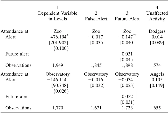
extended to 6 p.m. from July 1 to Labor Day. The Observatory is open from 2 p.m. to 10 p.m. Tuesday through Friday and 12:30 p.m. to 10 p.m. on Saturday and Sunday, but is open from 12:30 p.m. to 10 p.m. everyday during the summer. Both are located a short distance from downtown Los Angeles and attract sizeable crowds, averaging more than 4,500 attendees per day. These data are available from 1989–97, with descriptive statistics for each shown in Table 1.
Although focusing on two specific facilities limits generalizability, these data pro-vide several advantages over time use surveys. One, because they are administrative data, they are likely to be free of recall errors that often arise in survey data. Two, these data are available over a long period of time in which there is substantial var-iation in ozone levels, forecasts, and smog alerts. Three, the exact dates are available in the attendance data, allowing me to merge several files at the daily levels and use the regression discontinuity design. Therefore, this approach improves upon mea-surement, precision, and causality at the expense of generalizability.
The Zoo charges varying admission fees, so it also offers some breakdown of at-tendance by demographics to assess heterogeneity in responses to alerts. Separate daily attendance is available for adults, children younger than 2, children aged 2–12, and seniors aged 62 and older, with means for each presented in Table 1. Chil-dren and the elderly are two groups considered susceptible to the effects of ozone, so their responses may differ from adults.9Although this definition of susceptibility is not exhaustive, both groups are specifically targeted by air quality information. The Zoo also offers attendance for Greater Los Angeles Zoo Association (GLAZA) mem-bers. While the Zoo is both a tourist and local attraction, GLAZA members are typ-ically local residents who may be more aware of alerts and find it easier to switch activities.10Therefore, they are more likely to respond to alerts, providing one
ro-bustness check of the model.
I also collect data on attendance at baseball games (available in the ‘‘game logs’’ at www.retrosheet.org) for two major league baseball teams in SCAQMD: the Los Angeles Dodgers, who play a short distance form downtown Los Angeles, and the California Angels,11 who play in Anaheim, approximately 30 miles southeast of
8. The Zoo and Observatory are owned and operated by the City of Los Angeles.
9. Children’s responses to alerts could reflect state rules requiring schools to reschedule outdoor activities, but the analysis focuses almost exclusively on summer months when children are not in school and also includes a dummy variable for summer schedule.
10. GLAZA members pay an annual fee and do not pay an admission fee per visit.
Table 1
Summary statistics
A. Daily attendance
Mean Standard Deviation
Zoo (n¼1949) 4,766 3,160
Children <2 299 362
Children 2–12 766 774
Seniors 81 51
Adult 1,530 1,655
GLAZA members 718 538
Observatory (n¼1,770) 5,629 2,368
Dodgers (n¼574) 37,886 8,012
Angels (n¼655) 26,679 9,042
B. Daily asthma hospital admissions
Age Group Per SRA Per SCAQMD
5–19 0.369 9.007
20–64 0.737 17.995
65+ 0.292 7.165
C. Alert accuracy
Year Zoo SCAQMD
1989 16/6/9 169/56/89
1990 12/2/5 118/28/54
1991 20/4/8 142/34/50
1992 24/2/8 140/39/42
1993 10/2/1 84/23/20
1994 15/3/2 107/14/20
1995 7/0/1 32/3/5
1996 0/0/1 16/0/6
1997 0/0/0 3/0/1
Total 104/19/35 811/197/287
downtown Los Angeles. Attending a baseball game is a more sedentary activity than attending the Zoo or Observatory and most baseball games are played at night when ozone levels decrease, so I use attendance at games as a specification check. Average attendance from 1989–97, which includes advance ticket sales and purchases the day of the game, is over 37,000 for the Dodgers and 26,000 for the Angels. The sample size for both teams is considerably smaller than the Zoo and Observatory because the baseball season is shorter than the smog alert season and because games are not played every day in Southern California.
B. Health Outcomes
Data on health outcomes comes from a nonpublic version of the California Hospital Discharge Data (CHDD), which contains records for all individuals discharged from a hospital in the state. The nonpublic version contains the exact date of admission and the patients’ residential ZIP code, which are used to assign individuals to infor-mation, pollution, and weather. The principal diagnosis of the patient is used to iden-tify asthma admissions based on the International Classification of Diseases, 9th Revision, Clinical Modification (ICD-9–CM) codes. Because the effects of pollution and responses to information may vary by age, I use the age of the patient to separate admissions by age. Although an imperfect measure of health, asthma hospital admis-sions from the CHDD provide a large sample of data at a high frequency with de-tailed geographic residence.
Table 1 (continued)
D. Independent variables
Zoo SCAQMD
Variable Mean
Standard
Deviation Mean
Standard Deviation
Alert 0.053 0.225 0.071 0.257
Ozone one-hour (ppm) 0.078 0.038 0.082 0.043
Ozone one-hour if alert ¼ 1 0.129 0.037 0.149 0.046 Ozone one-hour forecast (ppm) 0.115 0.046 0.108 0.050 Maximum temperature
(degrees Fahrenheit)
82.15 9.70 81.91 10.84
Precipitation (inches) 0.218 1.617 0.200 1.546
Relative humidity (percent) 89.75 7.11 89.76 7.30
Average cloud cover sunrise to sunset (percent)
0.450 0.298 0.443 0.297
Resultant wind speed (mph) 5.66 2.37 5.70 2.37
For the dependent variable, I compute the daily number of hospital admissions for asthma in each SRA, also shown in Table 1. I compute asthma admissions for three age groups: 5–19, 20–64, and 65 and older.12The value of 0.369 for ages 5–19 in the first column indicates there are 0.369 hospital admissions per day for asthma per SRA, which translates into nine admits per day for all of SCAQMD, shown in the second column.
C. Air quality information
I collected forecasted ozone directly from theLos Angeles Timesfor the years 1989– 97. Since theLA Timesonly reports air quality forecasts for each AMA (although it receives forecasts for each SRA), the AMA is the finest geographic resolution for pollution information. For data on smog alerts, I obtained an administrative file from SCAQMD that contained dates when alerts were issued anywhere in the district but not the area it was issued for. Because there is considerable spatial variation in ozone levels throughout SCAQMD, I instead assign an alert to each AMA if the ozone fore-cast in that AMA (from theTimes) equals or exceeds 0.20 ppm, according to Equa-tion 1.13To verify the appropriateness of assigning alerts, I created an indicator for
whether an alert was issued anywhere in SCAQMD and compare it to the SCAQMD administrative file. The selection rule in Equation 1 is strictly followed: there are only seven inconsistencies of the 2,138 data points available over the period studied. Since alerts are forecasted, I assess their accuracy by using data on observed ozone for each AMA, also shown in Table 1. Of the 104 alerts issued in the AMA for the Zoo, fewer than 20 percent were correctly issued; conversely, on 35 days thee ozone surpassed 0.20 ppm but no alert was issued. Accuracy for the rest of SCAQMD is comparable to the AMA of the Zoo. If people track alert accuracy, the inaccuracy of alerts may be problematic for encouraging people to respond.14It is, however, use-ful for the regression discontinuity design: If scientists and meteorologists cannot distinguish between days above and below the threshold, then it is unlikely that indi-viduals can.
D. Pollution and weather
Daily pollution data is from the California Air Resources Board. There is approxi-mately one pollution monitor for ozone in each of the 38 SRAs, and roughly 20 for car-bon monoxide (CO) and nitrogen dioxide (NO2), two other pollutants necessary to
control for because of their correlation with ozone and potential health effects.15I as-sign pollution levels to the SRA based on the values for the monitor in that SRA and drop SRAs if no monitor is present for ozone. If an SRA does not have a monitor for CO or NO2, I assign pollution values from the nearest SRA with a monitor to preserve
12. I omit children younger than five because of difficulties in correctly diagnosing asthma at this age. 13. The ozone forecast is reported in PSI units, rather than ppm that observed ozone levels are recorded. Because the PSI is a nonlinear function of ppm, I convert the ozone forecast to ppm.
14. I estimated models that also included an indicator for whether alerts are issued correctly, and found no significant differences in the estimates.
sample size. I use measures of these pollutants that correspond with air quality stand-ards for the dates of the analysis.
Because weather is correlated with ozone levels and may directly affect time spent outside and health, I control for numerous weather variables obtained from the Surface Summary of the Day (TD3200) from the National Climatic Data Center. Using the 30 weather stations available in SCAQMD, I assign daily maximum and minimum temper-ature and precipitation to each SRA in an analogous manner to pollution. For maximum relative humidity, sun cover, and resultant wind speed, there is only one weather station in SCAQMD with a complete history of this variable (Los Angeles International Air-port), so I assign it to all SRAs within SCAQMD. These variables are also frequently missing, so to preserve sample size I impute the missing values using a best-subset re-gression with all other weather variables and ozone as covariates.
To assign information, pollution, and weather to individuals in the CHDD, I assign SRAs and AMAs to each individual using their ZIP code of residence, and merge the data by SRA or AMA and date. There are considerable disagreements over how to assign pollution from monitors to individuals. Using SRAs is justified on the grounds that SRAs were specifically designed to represent an area with common geography and pollution concerns, so there is a high degree of uniformity in ozone levels within an SRA. Each outdoor venue is linked to the pollution and weather station within its SRA by date as well.
IV. Conceptual Framework
A. Health Effects of Ozone
To fix ideas on measuring and interpreting the effect of pollution on health, assume the following relationship between asthma and ozone:
asthma¼fðozoneavoidance;SÞ ð2Þ
whereavoidanceis a measure of avoidance behavior, such as time spent outdoors, andSare all other factors that affect health, such as medical services, exercise, exist-ing health capital, and weather. Interactexist-ing ozone with avoidance behavior reflects exposure to pollution: ozone affects people only if they are exposed to it. For exam-ple, if ozone is 0.20 ppm and people spend no time outside (possibly because an alert is issued), then exposure to ozone is considerably less than if they spend time out-side.
Imagine two experiments, both of which hold fixedSbut differ in how they treat outdoor time. In the first experiment, which is analogous to controlled-human expo-sure experiments, individuals are randomly assigned into one of two rooms, each containing different levels of ambient ozone. Individuals can not respond to the amount of ambient ozone in the room (davoidance/dozone¼0), so their exposure to ozone is identical to the ambient level of ozone. Because of random assignment, the difference in outcomes across the two groups (dasthma/dozone) is a causal esti-mate of the biological effect of ozone on asthma.
levels of ambient ozone. In contrast to the first experiment, people can respond to the amount of ambient ozone in their location, so their exposure to ozone is not necessarily identical to the ambient level of ozone. Since these responses are not held fixed, the measured effect of ozone on asthma (dasthma/dozone¼dasthma/dozone+ dasthma/davoidancedavoidance/dozone) does not represent the biological effect. Because of random assignment, this is a causal estimate of the ‘‘behavioral’’ effect of ozone on asthma. If outdoor time is negatively correlated with ambient ozone lev-els, then the behavioral effect will represent a lower bound of the biological effect. If any responses to ambient ozone in the second experiment can be properly accounted for, the direct health effect from responding (dasthma/davoidancedavoidance/dozone) represents the ‘‘avoidance’’ effect. That is, it represents the effect from limiting exposure to ozone on asthma for a given level of ozone. Importantly, it can be used as an alternative way of examining whether ozone affects asthma—if people reduce their exposure to a pollutant and these causes an improvement in health, then the pollutant must affect health. Furthermore, accounting for avoidance behavior enables one to uncover the bio-logical effect of ozone on asthma.
B. Avoidance behavior16
Individuals may substitute between indoor and outdoor activities because they believe exposure to outdoor pollution affects health and because of the direct utility they re-ceive from spending time outside. People spend less time outside (increase avoidance behavior) when forecasted ozone increases if more time outside is worse for health when ozone is high, a reasonable condition because it is precisely what air quality in-formation conveys.17Susceptible people are more likely to respond to information if
avoidance behavior is more productive for them, also a reasonable condition. If responses to information vary by susceptibility, then the bias in estimates of the health effect of ozone from omitting avoidance behavior will vary by susceptibility as well.
Although susceptible individuals are more likely to respond to air quality information in general, they may be less likely to respond to smog alerts per se. Smog alerts are widely disseminated, so the cost of acquiring this information is nearly zero. All individuals— regardless of susceptibility—are encouraged to respond to alerts, so some unsusceptible individuals will respond to alerts if the expected benefits from responding outweigh the costs. Obtaining the ozone forecast, however, involves greater effort, so only those who benefit from avoiding ozone—the susceptible population—are likely to acquire that in-formation. Since smog alerts are determined by the ozone forecast, then smog alerts offer no additional information once the ozone forecast is obtained. Therefore, susceptible individuals are less likely to respond to an alert than unsusceptible individuals.
V. Estimation Strategy
There are two primary empirical objectives: to assess whether people respond to air quality information and, if they respond, to assess the bias from
16. Contact the author for a full derivation of the predictions described in this section.
incorporating these responses. Although the empirical models are nested theoreti-cally, I separately elaborate on empirical strategies for each equation because: (1) the data do not fully overlap since I only observe outdoor behavior for two locations in SCAQMD but hospital admissions for all of SCAQMD and (2) empirical concerns unique to each model requires different identification strategies.
A. Avoidance behavior
To estimate the effect of air quality information on attendance at each outdoor loca-tion, I focus on estimating the impact of smog alerts only and use the ozone forecast to identify the effect of smog alerts. Since alerts are a deterministic function of the forecasted ozone, as indicated in Equation 1, forecasted ozone fully governs the alert selection rule and makes it possible to leverage a regression discontinuity (RD) de-sign. If days just below forecast ozone levels of 0.20 ppm are otherwise identical to days just at or above 0.20, then the discontinuity in attendance that occurs at 0.20 ppm represents the causal effect of alerts. If people directly respond to the ozone forecast, this does not invalidate the empirical strategy—it will simply reduce the ef-fect of alerts on attendance. Therefore, this design assesses whether people respond to the more simplistic and readily available information contained in alerts condi-tional on the continuous index being available.
To implement the RD, I estimate the following equation:
logðattendancetÞ ¼alertta1+gðozoneft;a2Þ+Xta3+Mta4+fðtÞ+et
ð3Þ
wherealertt is a dummy variable indicating whether a smog alert is issued in the AMA of the outdoor facility at dayt,gis a function that relates the ozone forecast (ozonef)to attendance, andetis an error term.Xtare meteorological and pollution variables that affect quality of the day. Mt are holiday, summer schedule, and day of week dummies to account for changes in leisure time.f(t)is a set of year-month dummy variables to account for both seasonal and temporal patterns in solar radia-tion, polluradia-tion, and weather. If a1 < 0, this indicates outdoor attendance decreases when alerts are announced. Because the Observatory is open during the evening when ozone levels are lower and responses may be smaller there than at the Zoo, I estimate this model separately for both places.18
To allow for a flexible specification ofg, I begin by estimating a specification lin-ear in ozone forecast, as graphical evidence below suggests is plausible. Addition-ally, I control for g nonparametrically by specifying a dummy variable for each value of the ozone forecast, but omit the smog alert variable. To infer the impact of alerts, I use the change in coefficients around the alert threshold by comparing the dummy variable onozonef¼0.19 toozonef¼0.20 ppm. If the dummy variable above the alert threshold is lower than the one below the alert threshold, this implies a decrease in attendance in response to alerts.19
18. Since the covariate (ozone forecast) that determines the treatment (smog alert) is discrete, I compute standard errors clustered on each value of forecasted ozone (Card and Lee 2006).
While it is impossible to know whether the unobservables are identical across alert status, I examine how well the observable covariates balance across alert status. Fig-ure 1 shows a plot of three likely influential covariates (temperatFig-ure, humidity, and CO) against ozone forecast levels. All three covariates evolve smoothly throughout this plot, suggesting they are unaffected by smog alerts. Given the observed factors balance, then it is more reasonable to believe the unobserved factors do as well.
As preliminary evidence that people respond to alerts, average attendance at the Zoo is also plotted in Figure 1. Focusing on the observations near 0.20 ppm, atten-dance is generally increasing in forecasted ozone prior to 0.20 ppm. At 0.20 ppm, the point at which an alert is issued, attendance sharply drops. After that, attendance remains increasing in forecasted ozone, but is generally lower than attendance below 0.20 ppm. This jump in attendance at the alert threshold, which is larger than any other jump in attendance, provides the first piece of evidence that people respond to smog alerts.
Two additional assumptions necessary to obtain unbiased estimates ofa1 is that (1) alert status is not updated once actual levels of ozone are realized and (2) there are no supply-side effects. Despite the temptation to continuously update alert status, officials at SCAQMD indicate this is highly unlikely because of flaws inherent in detecting and disseminating an alert as it occurs.20In terms of supply side effects,
facilities do not lower their price to entice customers or keep animals inside to pro-tect their health on alert days, suggesting this assumption is likely to be satisfied. It is possible, however, that a more crowded atmosphere provides less enjoyment because of longer waiting times, for example. If an alert reduces crowding so that unsuscep-tible people increase demand for these outdoor attractions, this will result in a down-ward bias ina1.
Figure 1
Zoo Attendance and Covariates by Ozone Forecast
B. Health Effects of Ozone
To estimate the effect of ozone on health, one would ideally focus on a more detailed version of Equation 2 that includes lagged values of ozone, outdoor time, and other appropriate variables. This is not feasible because the data with health outcomes cov-ers all of SCAQMD while the data for outdoor time is not at the individual level and only covers two particular places. Instead, I substitute the factors that affect outdoor time into Equation 2 to estimate the following reduced form relationship:
asthmasat¼ +
wheres,a, and tindexes SRA, AMA, and time, respectively, andvsat is the error term.21his the number of hospital admissions per day in each SRA. To remain con-sistent with previous ozone time-series studies that often found effects up to four days after exposure (Environmental Protection Agency 2006), I include four lags of ozone, information, and weather, but also assess sensitivity to alternative amounts of lags.X, M,andf(t)are the same as Equation 3, except I also include smog alerts and the ozone forecast in levels inXto capture nuance effects associated with alerts being issued, such as individual over-reactions to alerts or hospitals increased will-ingness to admit patients because of an alert.ssis an SRA fixed effect that accounts for observed and unobserved determinants of health within an SRA. Therefore, I compare changes in ozone levels and information with changes in hospitalizations within each month of the year and within an SRA.
The primary test of this analysis focuses on whether accounting for avoidance behavior affects estimates the biological effect of ozone on health. Instead of compar-ing the effect of each lag separately, I focus on the overall effect of ozone by comput-ing the sum of the effect of ozone across all lags, +ð@asthmasat=@ozonesat2jÞ ¼
+p11j +alertt2jp12j +ozonet2jf p j
13
. If people respond to information about pollution
and ozone affects health, then including smog alerts and the ozone forecast should in-crease estimates of the effect of ozone. To formally test this hypothesis, I estimate Equation 4 both with and without controls for information about risk, and compare estimates via a Hausman test (Hausman 1978).22
The identification of ozone comes from daily variation in ozone levels within each year and month and within an SRA. To highlight this variation in ozone, Figure 2 plots the mean level of ozone for each day of the year. Immediately evident is the strong daily variation in ozone, which is likely to be orthogonal to diet, exercise,
21. Smog alerts and the air quality forecast are included in levels in the vectorX, described below. Al-though this equation should also contain ozone interacted with the other covariates (XandM), I omit the additional interactions to simplify exposition. Results with complete interactions, however, are nearly identical to results from this specification.
22. The Hausman test statistic is given by(gs-gl)’*½var(gl) – var(gs)-1* (gs-gl)
;x2(q) wheregsis the
estimated effect of ozone when excluding information from Equation 4,glis the estimated effect of ozone
health care choices, pre-existing health stock, and numerous other factors that affect asthma hospital admissions. This figure also demonstrates the strong seasonal pat-terns in ozone that are necessary to account for because behavior and environmental conditions change throughout the year as well
In order to obtain precise estimates of the parameters of interest, it is essential that there is enough variation in ozone levels independent of seasonality, weather, copol-lutants, and all other variables included in these regressions. Figure 3 plots the mean residual variation in ozone for each day of the year after adjusting forX, M, year-month dummies, and SRA fixed effects. This figure demonstrates substantial residual variation in ozone that is constant throughout the year, indicating seasonality is accounted for and ample variation for obtaining precise estimates.
A concern with using daily variation in ozone is the factors that drive this varia-tion—weather and ozone precursors—may directly affect health and not be observed inX.23With respect to weather, I control for temperature and sun cover—the two meteorological factors that affect ozone formation—directly in these regressions (as well as several other weather variables). Furthermore, I demonstrate below that estimates of the effect of ozone are insensitive to excluding all weather variables, suggesting confounding from weather is not a major concern.
With respect to ozone precursors (NOx and VOCs), I can not directly include them in regression models because they are generally unavailable at the same level of de-tail, but it is unclear whether to control for them even if they are available. On one hand, these pollutants are not believed to be directly related to asthma, so any effect they might have on asthma is through their effect on ozone, which would dampen the estimated effect of ozone on health. On the other hand, the sources of NOx and VOC emissions may emit other pollutants that affect health. For example, automobiles emit benzene, which has been linked with asthma, in addition to NOx. Although I can not include all copollutants in the empirical models, I include CO and NO2—two
criteria pollutants linked with short-term respiratory health effects—and also demon-strate results are insensitive to excluding these copollutants.
Figure 2
Variation in One-hour Ozone by Day of Year
As described in the conceptual framework, assessing the direct effect on informa-tion on asthma in Equainforma-tion 4 can be used as another test for understanding the health effects of ozone. If people respond to informationand information has a negative effect on asthma hospitalizations, this implies ozone must affect health. For example, if individuals respond to alerts by reducing their exposure to ozone and their health improves, then ozone must affect health. Rather than focus on specific lags, I also use the sum across all lags: +ð@asthmasat=@alertsat2jÞ ¼+ ozonet2jpj12
;
+ð@asthmasat=@ozonefsat2jÞ ¼+ðozonet2jp j
13Þ and jointly test whether the two
parameters are different from zero. Smog alerts are identified by including the ozone forecast, akin to the RD design linear in forecasted ozone, which evidence below indicates this is a reasonable approximation forg. The ozone forecast is only iden-tified if all factors that affect the ozone forecast, as specified in Equation 1, are ob-served in Equation 4. Although more tenuous than the assumption for the effect of smog alerts, it is a plausible assumption given the extensive controls for weather, so-lar radiation, and lagged ozone.
VI. Do People Respond To Smog Alerts?
The first set of regression results, shown in Table 2, provides further evidence that people respond to smog alerts by decreasing outdoor activities. There is a separate panel for each outdoor facility, and each panel includes results from four specifications to gauge the sensitivity of estimates to both potential confounding and functional form assumptions of the RD. The odd numbered columns omit several variables likely to affect the demand for outdoor activities (precipitation, wind, hu-midity, observed ozone, carbon monoxide, and nitrogen dioxide), while the even numbered columns include them.24Columns 1 and 2 use a linear specification for
Figure 3
Residual Variation in One-hour Ozone by Day of Year
the RD and Columns 3 and 4 are nonparametric estimates that specify a dummy vari-able for each forecasted ozone value.
Results for the Zoo are shown in Panel A. Columns 1 and 2 show a statistically significant drop in attendance of 15 percent both with and without the additional weather and air quality covariates. The nonparametric results in Columns 3 and 4 in-dicate that smog alerts reduce attendance between 12 and 13 percent, quite similar to the parametric estimates. Moreover, the results are almost completely unaffected by excluding several important covariates, which is notable given that weather and ob-served ozone are important predictors of outdoor activities. This suggests that these variables evolve smoothly around the discontinuity, so the change in attendance at the discontinuity represents the causal effect of smog alerts.
Results for the Observatory, shown in Panel B, also show a decline in attendance from smog alerts. Attendance declines by roughly 3 percent in the parametric model, though statistically insignificant. In the nonparametric specification, there is a statis-tically significant drop in attendance of 6 percent, which is larger than the parametric estimates. All estimates are also insensitive to including the weather and pollution variables. These results suggest a response to alerts, with the smaller magnitude than the Zoo consistent with the Observatory including night hours when ozone levels typically decrease.
Table 2
Regression estimates of smog alerts on attendance
1 2 3 4
A. Dependent variable¼log(daily attendance) at Los Angeles Zoo
Alert 20.148** 20.150** 20.122** 20.129** [0.036] [0.040] [0.013] [0.014] Functional form of ozone forecast Linear Dummy Variables
Controls for weather N Y N Y
Observations 1,949 1,949 1,949 1,949
B. Dependent variable¼log(daily attendance) at Griffith Park Observatory
Alert 20.032 20.031 20.061** 20.059**
[0.023] [0.022] [0.013] [0.014] Functional form of ozone forecast Linear Dummy Variables
Controls for weather N Y N Y
Observations 1,770 1,770 1,770 1,770
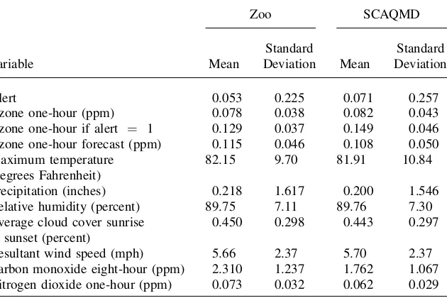
I provide several sensitivity analyses to assess the robustness of these results. If the costs of avoiding these outdoor activities are lower for local residents, either because they are more aware of information or have lower costs of substitution, then they should display larger responses to alerts. Using the attendance breakdown at the Zoo, I explore how GLAZA members respond to alerts. Shown in Column 1 of Table 3, GLAZA mem-bers reduce attendance by 19 percent, which is larger than the total attendance response. Given that GLAZA members are more likely to be local residents, this conforms to expectations that locals show a greater response to alerts than other attendees.
More susceptible people are more likely to display avoidance behavior, but they may be less likely to respond to alerts if they obtain the continuous ozone forecast. To assess this, I estimate Equation 3 for the Zoo separately for children and the elderly, two sus-ceptible groups. The results, shown in Columns 2–4 of Table 3, indicate responses be-tween 19 and 24 percent for children and seniors, also larger than the overall response. Although this basic classification of susceptibility is not sufficient for capturing those with a history of respiratory illness, it captures two major groups targeted by air quality information. In general, these results suggest the more simplified information con-tained in the alerts is valued by potentially susceptible populations.
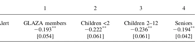
I also provide several specification tests for this model, shown in Table 4. As a first test, I estimate regressions with the dependent variable in levels rather than logs, which holds constant the number of attendees, rather than percent of attendees, af-fected by alerts. Shown in Column 1, the implied percentage drop in attendance is comparable in magnitude to the main results: Zoo attendance drops by 10 percent and Observatory attendance by 3 percent.
Second, I provide a falsification test by testing for a discontinuity where one should not exist.25Following Imbens and Lemiuex (2007), I use the sub-sample with no smog alerts (ozone forecasts less than 0.20 ppm), which avoids estimating a regression where a known discontinuity exists, and create an artificial discontinuity at the median ozone forecast, which maximizes the power of the test to find jumps.26The results, shown in Column 2, are not statistically significant, providing support for the model.
As a third check, I include future alerts in Equation 3. People cannot respond to a forecasted alert before it occurs, so finding an effect would suggest misspecification. If people use a naı¨ve version of Equation 1 to forecast ozone on their own, however, then they may anticipate future smog alerts by increasing current outdoor activities, suggesting a positive coefficient on future alerts. Therefore, only a negative coeffi-cient on future alerts would suggest misspecification. The results, shown in Column 3 of Table 4, indicate a positive but statistically insignificant effect from future alerts for both facilities, hinting people may anticipate future smog alerts. Furthermore, the effects from contemporaneous alerts are unaffected by the inclusion of future alerts. For a final specification check, I estimate the regression using an outcome that should not be affected by smog alerts. One concern with the evidence presented thus far is that people may respond to alerts out of altruistic rather than health concerns by driving less so as to not further contribute to pollution on days already considered highly polluted. Therefore, people may reduce visits to specific outdoor attractions but not limit total time outside, implying a decrease in outdoor attendance is not
evidence of avoidance behavior. Since attending baseball games is a sedentary activ-ity and typically at night when ozone levels are lower, attendance at Dodgers and Angels games should not be affected by alert status. Shown in Column 4 of Table 4, smog alerts are not statistically significant for both teams, and the large point es-timate for the Angels suggests, if anything, an increase in attendance, which is con-sistent with lower ozone levels at night.27 This finding helps to substantiate the
overall evidence that people are displaying avoidance behavior in response to infor-mation about pollution.
Overall, these estimates suggest a significant drop in attendance from an alert. The results are extremely insensitive to functional form assumptions and potential con-founding, and are of the same order of magnitude despite coming from distinct sour-ces, making it unlikely these results are due to sampling variability or general misspecification. The results suggest people respond to smog alerts by reducing time spent outdoors.
VII. The Health Effects of Ozone
Given the evidence that people respond to these alerts, I now turn to whether this impacts estimates of the effect of ozone on health by presenting both graphical and regression analyses.
A. Graphical analysis
The main finding of this analysis is depicted in Figure 4 (a and b). This figure is a nonparametrically smoothed scatter plot of regression-adjusted asthma hospitaliza-tions against once lagged observed ozone levels.28I focus on one lag here because previous studies have found the one-day lag to have the largest effect on hospital
Table 3
Regression estimates of smog alerts on Zoo attendance by demographic
1 2 3 4
Alert GLAZA members Children <2 Children 2–12 Seniors 20.193** 20.222** 20.236** 20.194**
[0.054] [0.061] [0.061] [0.042]
Notes: See notes to Table 2. There are 1949 observations in all models. The specification in each column is comparable to the linear RD model from Column 2 in Table 2.
27. Results are nearly identical when using only night games. As an additional test, if people drive less in response to alerts, then CO levels—a proxy for traffic because it primarily comes from automobiles— should fall at the alert threshold. As shown in Figure 2, however, CO evolves smoothly through the alert threshold, rejecting the altruism effect.
admissions (Environmental Protection Agency 2006), though regressions below con-trol for several lags simultaneously. To assess the impact of avoidance behavior, I plot two separate lines. The first line ignores avoidance behavior by plotting asthma and observed ozone levels for all days regardless of whether a smog alert is issued. The second line accounts for avoidance behavior by limiting the plot to days where no smog alerts occur—so people could not have displayed avoidance behavior in re-sponse to an alert. If people respond to alerts and ozone affects health, then the sec-ond line should be higher than the first line.
The results for children (Figure 4a) confirm the importance of avoidance behavior. For lower levels of ozone, the two lines mirror each other, which is as expected be-cause alerts, and therefore avoidance behavior, are unlikely at such low levels of realized ozone. Once ozone crosses 0.1 ppm and smog alerts become more com-mon, however, the two lines diverge.29The relationship between ozone and hospital-izations flattens out considerably when ignoring smog alerts, which is consistent with avoidance behavior: as pollution levels rise, individuals protect themselves by reduc-ing exposure, so increases in ambient ozone do not lead to increases in illness.
Table 4
Specification checks of estimates of smog alerts on attendance
1
2 3
4 Dependent Variable
in Levels False Alert Future Alert
Unaffected Activity
Attendance at Zoo Zoo Zoo Dodgers
Alert 2476.194* 20.017 20.147** 0.014
[201.902] [0.035] [0.040] [0.089]
{0.100}
Future alert 0.031
[0.045]
Observations 1,949 1,845 1,898 574
Attendance at Observatory Observatory Observatory Angels
Alert 2146.114 20.016 20.034 0.105
[90.748] [0.032] [0.023] [0.149]
{0.026}
Future alert 0.032
[0.031]
Observations 1,770 1,671 1,723 655
Notes: See notes to Table 2. The specification in each column is comparable to the linear RD model from Column 2 in Table 2. The value in braces in Column 1 represents the percentage change in attendance. False alert is assigned at the median ozone forecast (0.11 ppm) for the subsample with ozone forecast < 0.20 ppm.
Accounting for smog alert status, however, paints an entirely different picture; it shows a positive and linear relationship between ozone and asthma throughout the entire range of ozone. As ozone increases and alerts become more common, the line accounting for avoidance behavior is considerably higher than the one ignoring it. Although both lines support an effect of ozone on health, the line ignoring behavior substantially understates the effect.
The results for adults (Figure 4b) suggest avoidance behavior does not bias esti-mates for this age group. The two lines are nearly indistinguishable from each other, showing a positive, linear relationship between ozone and asthma throughout the
Figure 4a
Adjusted Asthma Hospital Admissions by Age on Lagged Ozone by Alert Status, Ages 5-19
Figure 4b
entire range of ozone. This suggests adults do not engage in avoidance behavior in response to an alert, which is consistent with results from Table 3 indicating that chil-dren and the elderly Zoo attendees show greater responses to alerts than adults.
B. Regression results
Regression estimates (shown in Table 5), which extend the graphical analysis by allowing for contemporaneous and several lags of ozone and other environmental confounders, support the graphical relationship from Figure 4. For children, esti-mates of the effect of ozone that omit air quality information in Column 1 indicate that a 0.01 ppm increase in the five-day average ozone leads to a statistically signif-icant 1.09 percent increase in hospital admissions. When controlling for smog alerts and the ozone forecast, estimates in Column 2 indicate a 0.01 ppm increase in the five-day average ozone leads to a statistically significant 2.88 percent increase in hos-pital admissions, which is 2.6 times larger than estimates that ignore information, a statistically significantly difference according to the Hausman test. Furthermore, alerts have a statistically significant and negative effect on hospitalizations, suggesting a reduction in exposure to ozone via smog alerts improves health. These results are
Table 5
Regression estimates of ozone and avoidance behavior on asthma hospitalizations by age
1 2 3 4 5 6
Age 5–19 Age 20–64 Age 65+
Ozone (sum of lags) 0.401* 1.061** 1.356** 1.532** 0.558** 0.776** [0.185] [0.245] [0.254] [0.335] [0.158] [0.208] {1.09} {2.88} {1.84} {2.08} {1.91} {2.66}
Hausman test (x2) 20.45 0.74 2.92
Probability >x2 0.00 0.39 0.09
Alerts (sum of lags) 20.162**
20.039 20.014
[0.057] [0.078] [0.049]
PSI (sum of lags) 0.013 20.019 20.037
[0.031] [0.042] [0.026]
F(alerts, PSI)¼0 5.41 0.59 2.16
Probability >F 0.00 0.55 0.12
consistent with the hypothesis that families protect this vulnerable segment of the pop-ulation, and this behavior affects the estimated relationship between ozone and health. Also consistent with the graphical results, estimates for adults ages 20–64 are un-affected by controls for information about pollution, shown in Columns 3 and 4. Esti-mates of the effect of ozone are statistically significant in both specifications, and controlling for information does not affect these estimates according to the Hausman test. Estimates with controls for information indicate a 0.01 ppm increase in the five-day average ozone leads to a 2.08 percent increase in hospital admissions, which is slightly smaller than the effect on children. Consistent with information not impact-ing the estimates for ozone, information has no direct effect on health. This suggests adults do not respond to this information in sufficient volume to affect the estimated relationship between ozone and health.
For the elderly, shown in Columns 5 and 6, the effect of ozone is statistically sig-nificant in both specifications. Estimates are 40 percent larger with controls for both alerts and the ozone forecasts (Column 6) than estimates without controls for infor-mation (Column 5), which is significantly different at the 10 percent level. The effect of a 0.01 ppm increase in the five-day average ozone on asthma admissions is 2.66 percent, which is close to the effect for children. Although neither source of in-formation is statistically significant at conventional levels, the ozone forecast is sta-tistically significant at 15 percent, suggesting the ozone forecast is the more important piece of information for the elderly. Overall, these results imply the elderly display avoidance behavior, though its impact on estimates is smaller than the impact for children.
To gauge the magnitude of these effects, I calculate the savings in asthma hospital costs for children only from a uniform 0.01 ppm decrease in the five-day average ozone in all SRAs in SCAQMD using estimates from Columns 1 and 2 in Table 5. Using estimates from Column 1 and valuing an asthma admission at the mean hos-pital bill for asthma ($7301), a 0.01 ppm decrease yields savings of roughly $157,727 per smog alert season.30Controlling for information about pollution increases this
estimate considerably to $417,717.31The difference of roughly $260,000 between these estimates for children suggest the importance of accounting for avoidance be-havior, but it represents a lower bound of this difference because it ignores any direct effects on well-being not included in hospital costs and it ignores other health epi-sodes that do not result in asthma hospitalizations. Therefore, the estimated differ-ence in costs understates the full differdiffer-ence in social benefits associated with reductions in ozone levels.
C. Sensitivity Analyses
In Table 6, I assess the sensitivity of estimates to the number of lags included in the regression. I begin with a model containing only contemporaneous ozone, informa-tion, and weather, and then consecutively add one lag at a time, with the final spec-ification including six lags. For children, in the model without controls for avoidance
behavior, the effect of ozone is monotonically increasing from zero to three lags, and levels out after that, generally consistent with prior evidence. With controls for avoidance behavior, the effect of ozone is monotonically increasing even through lag 6, suggesting more lags than is typically used may be necessary for capturing the full health effects of ozone on children. For adults and the elderly, three and four lags appears to sufficiently capture all of the health effects, respectively, regardless of whether avoidance behavior is controlled for.
In Table 7, I present a series of specification checks to assess the likelihood of time-varying unobserved heterogeneity. As previously mentioned, ozone is corre-lated with weather and other pollutants that may affect health but not be fully cap-tured in these models. As a crude test, I estimate models that do not control for weather and other pollutants. If estimates are insensitive to excluding these variables, this increases confidence that there is no remaining confounding. These estimates, shown in Panel A (excluding weather) and B (excluding copollutants) of Table 7, confirm that the effects of ozone are generally unaffected by these variables, lending support to the empirical methodology.
I also estimate models using only emergency room (ER) admissions as the depen-dent variable. Hospital admissions for asthma can be prearranged and may not reflect the effect of exposure to ozone, while ER admits, which are roughly 60 percent of all hospital admits for asthma, are unplanned episodes that are more likely to be an immediate reaction to ozone. The results, shown in Panel C of Table 7, indicate
Table 6
Lag sensitivity of regression estimates of ozone on asthma hospitalizations by age
1 2 3 4 5 6
Age 5–19 Age 20–64 Age 65+
Ozone (0 lags) 0.177 0.176 0.536 0.433 0.203 0.307
[0.121] [0.144] [0.166] [0.198] [0.103] [0.123]
Ozone (1 lag) 0.308 0.420 0.870 0.843 0.266 0.380
[0.142] [0.177] [0.195] [0.243] [0.121] [0.151]
Ozone (2 lags) 0.340 0.625 1.223 1.354 0.358 0.498
[0.159] [0.205] [0.218] [0.281] [0.136] [0.175]
Ozone (3 lags) 0.468 0.976 1.237 1.325 0.419 0.518
[0.173] [0.228] [0.237] [0.313] [0.148] [0.194]
Ozone (4 lags) 0.401 1.061 1.356 1.532 0.558 0.776
[0.185] [0.245] [0.254] [0.335] [0.158] [0.208]
Ozone (5 lags) 0.425 1.255 1.371 1.521 0.543 0.718
[0.196] [0.262] [0.270] [0.360] [0.168] [0.224]
Ozone (6 lags) 0.462 1.411 1.203 1.235 0.571 0.729
[0.208] [0.280] [0.285] [0.384] [0.177] [0.238]
estimates are insensitive to this alternative measure—although coefficients are smaller, it has a comparable percentage effect on ER admissions as hospital admis-sions.
As a general specification check, I add future pollution levels, information, and weather to the model. Ozone and information in the future cannot affect health today, so any effect would suggest misspecification of the model. To maintain balance with the lagged structure of the model, I add five leads of ozone and information along with the appropriate interaction terms, and separately test the joint significance of the biological and avoidance effect. The results, shown in Panel D of Table 7, reveal quite comparable
Table 7
Specification checks of estimates of ozone and avoidance behavior on asthma hospitalizations by age
1 2 3 4 5 6
Age 5–19 20–64 65+ 5–19 20–64 65+
A. No Weather B. No Copollutants
Ozone (sum of lags) 1.116*** 1.524** 0.742** 1.298** 1.582** 0.780**
[0.237] [0.325] [0.202] [0.240] [0.329] [0.204]
{3.03} {2.07} {2.55} {3.52} {2.15} {2.68}
Alerts (sum of lags) 20.166** 20.038 20.012 20.180** 20.045 20.014
[0.057] [0.078] [0.048] [0.057] [0.078] [0.049]
PSI (sum of lags) 0.013 20.021 20.038 0.023 20.012 20.035
[0.030] [0.041] [0.025] [0.030] [0.042] [0.026]
F(alerts, PSI)¼0 5.76 0.63 2.24 6.03 0.51 1.96
Probability >F 0.00 0.53 0.11 0.00 0.60 0.14
C. ER Admissions D. Future Ozone and Information
Ozone (sum of lags) 0.787** 1.052** 0.500** 1.020** 1.719** 0.831**
[0.178] [0.273] [0.158] [0.277] [0.384] [0.238]
{2.14} {1.43} {1.71} {2.77} {2.33} {2.85}
Alerts (sum of lags) 20.073 20.003 0.012 20.105 20.038 20.049
[0.042] [0.064] [0.037] [0.062] [0.086] [0.054]
PSI (sum of lags) 20.013 20.010 20.022 20.018 20.020 20.025
[0.022] [0.034] [0.020] [0.036] [0.049] [0.031]
F(alerts, PSI)¼0 3.79 0.09 0.71 3.29 0.46 1.92
Probability >F 0.02 0.91 0.49 0.04 0.63 0.15
Future ozone
Probability >F 0.86 0.79 0.67
effects of ozone and information as in Table 5 for all ages and no statistically significant effect from future alerts and ozone, providing general validation to the specification.
VIII. Conclusion
This paper finds that individuals in Southern California respond to in-formation about pollution by reducing time spent outside, and this significantly impacts estimates of the relationship between ozone and health for susceptible pop-ulations. If people change their behavior in response to this information, this action must have some costs to them. Given that providing information about pollution is a growing part of environmental policy,32measuring these costs is essential for
design-ing optimal policy and should be a focus of future research.
There are two important caveats to this study. First, Southern California has a unique history of smog and ozone, so the results may not necessarily generalize to other contexts. Although numerous cities provide various types of air quality fore-casts, they are typically less publicized than in Southern California. Furthermore, forecasting pollutants other than ozone is inherently more difficult, so information is less prevalent and reliable for other pollutants. In both cases, less information leads to less avoidance behavior, and less potential bias in estimates.
The second caveat is there may be additional sources of private information about pollution. Although ozone is not directly visible, it is a major component of smog, which is visible. There is no evidence to indicate whether people respond to this in-formation, but if the bias from omitting this information is in the same direction as the bias from omitting public information, then current estimates of the biological effect would remain underestimates of the true effect.
References
Ahituv, Avner, V. Joseph Hotz, and Tomas Philipson. 1996. ‘‘The Responsiveness of the Demand for Condoms to the Local Prevalence of AIDS.’’Journal of Human Resources 31(4):869–97.
Bell, Michelle, Aidan McDermott, Scott Zeger, Jonathan Samet, and Francesca Dominici. 2004. ‘‘Ozone and Short-Term Mortality in 95 U.S. Urban Communities, 1987–2000.’’ Journal of American Medical Association292:2371–78.
Bresnahan, Brian, Mark Dickie, and Shelby Gerking. 1997. ‘‘Averting Behavior and Urban Air Pollution.’’Land Economics73:340–57.
Brunekreef, Bert, and Stephen Holgate. 2002. ‘‘Air Pollution and Health.’’Lancet 360:1233–42.
Card, David, and David Lee. 2006. ‘‘Regression Discontinuity Inference with Specification Error.’’ NBER Technical Working Paper #322.
Chang L., Petros Koutrakis, Paul Catalano, and Helen Suh. 2000. ‘‘Hourly Personal Exposures to Fine Particles and Gaseous Pollutants.’’Journal of the Air and Waste Management Association50(7):1223–35.