Age, Women, and Hiring
An Experimental Study
Joanna N. Lahey
a b s t r a c t
As baby boomers reach retirement age, demographic pressures on public programs may cause policy makers to cut benefits and encourage employment at later ages. But how much demand exists for older workers? This paper reports on a field experiment to determine hiring conditions for older women in entry-level jobs in two cities. A younger worker is more than 40 percent more likely to be offered an interview than is an older worker. No evidence is found to support taste-based discrimination as a reason for this differential, and some suggestive evidence is found to support statistical discrimination.
I. Introduction
As the baby boom cohort reaches retirement age, social programs such as Social Security and Medicare face looming funding crises. One often sug-gested solution is to encourage older workers to remain in the labor force, so that benefits can be cut without compromising living standards (Burtless and Quinn 2001, 2002; Diamond and Orszag 2002). Not only are people living longer, but sev-eral studies suggest that today’s 70-year-olds are comparable in health and mental
Joanna N. Lahey is an assistant professor of public policy at Texas A&M University. She thanks the MIT Shultz fund, NSF Doctoral Dissertation Grant # 238 7480, the NSF Graduate Research Fellowship, and National Institute on Aging NBER Grant # T32- AG00186 for funding and support. Special thanks also goes to Mike Baima, Lisa Bell, Faye Kasemset, Jennifer La’O, Dustin Rabideau, Vivian Si, Jessica A. Thompson, and Yelena Yakunina for excellent research assistance. The author thanks David Wilson for expertise on the St. Petersburg area and Barbara Peacock-Coady for information on older labor market entrants and reentrants. Thanks also go to Liz Oltmans Ananat, Josh Angrist, David Autor, M. Rose Barlow, Melissa A. Boyle, Norma Coe, Dora L. Costa, Mary Lee Cozad, Michael Greenstone, Chris Hansen, Todd Idson, Byron Lutz, Sendhil Mullainathan, Edmund Phelps, John Yinger, and members of the MIT public finance and labor lunches, the NASI annual conference, and the Boston College Center for Aging and Work seminar for insightful comments. The author claims any errors as her own. The data used in this article can be obtained beginning August 2008 through July 2011 from Joanna N. Lahey, 4220 TAMU, College Station, TX 77843-4220, jlahey@nber.org
[Submitted September 2006; accepted March 2007]
ISSN 022-166X E-ISSN 1548-8004Ó2008 by the Board of Regents of the University of Wisconsin System
function to 65-year-olds from 30 years ago (Schaie 1996; Baltes, Reese, and Nessel-roade 1988). Many older Americans also may need to work even if Social Security benefits are not cut because they lack adequate retirement savings (Bernheim 1997). This lack of savings is especially acute for older widows, who suffer an average 30 percent drop in living standards upon widowhood and are more likely to be living in poverty than are other groups (Holden and Zick 1998; Favreault and Sammartino 2002).
Will older people be able to find work? Economists generally assume that labor force nonparticipation is voluntary for those in good health, so only supply-side factors come into play in policy discussions. This labor market experiment evaluates potential demand-side barriers to older women’s finding employment by exploring the hiring behavior, specifically the interviewing behavior, of firms that are seeking entry-level or close-to-entry-level employees. Although a number of sociology and psychology studies have directly examined age discrimination, these studies typi-cally present a human resources manager (or worse, a group of undergraduate psychology students) with two resumes, one of an older worker and one of a younger worker, and ask which the manager would be more likely to hire (for example, Nelson 2002). In contrast, this experiment analyzes real rather than hypothetical choices by businesses that do not know they are being studied.
The Age Discrimination in Employment Act (ADEA), implemented in 1968 and enforced in 1978, covers workers age 40 and up in firms with 20 or more employees, with a few exceptions.1This law prohibits discrimination based on age against older
workers through hiring, firing, and failure-to-promote mechanisms. Since it is more difficult for workers to determine why they failed to receive an interview than it is for workers to determine why they have been fired, firms that wish to retain only a certain type of worker without being sued would prefer to discriminate in the hiring stage rather than at any other point of the employment process. If discrimination in the hiring stage is going to occur, it is reasonable to expect that firms will do it as early in the hiring process as possible, specifically in the decision whether or not to interview.
My study examines the entry-level or close-to-entry-level labor market options for women ages 35 to 62 in Boston, Massachusetts and St. Petersburg, Florida. I send pairs of resumes to employers in these two cities and measure the response rates by age, as indicated on each resume by date of high school graduation. I find evi-dence of differential interviewing by age in these two labor markets. A younger worker is 42 percent more likely than an older worker to be offered an interview in Massachusetts and 46 percent more likely to be offered an interview in Florida. Because of the limited number of positions available, these differences in offer rates imply welfare losses for older job seekers.
In addition, I explore reasons for differential responses to resumes by age in several ways. Economic theory generally distinguishes between two major types of discrimination: statistical discrimination and taste-based discrimination. Statistical
1. Although the ADEA covers people older than 40, the majority of people who utilize the law are older than 50. Psychology studies suggest that firms most value workers in their 30s (Nelson 2002); if the law covered only workers aged 50 and older, firms could conceivably choose to do mass firing of 49-year olds and still be within the law. Firing 39-year olds in order to avoid lawsuits from 40-year olds may seem less attractive.
discrimination occurs when an individual is judged based on group characteristics. This form of discrimination is generally thought to be efficient for employers in cases of imperfect information (Arrow 1972).2 For example, if, in general, it is true that older workers take longer to learn unfamiliar tasks, then an employer may be reluc-tant to hire an older worker because testing each older applicant for ability to learn is costly. This efficient form of discrimination differs from taste-based discrimination, which occurs when an employer, a set of employees, or a customer base gets disutil-ity from working with individuals from a specific group. Taste-based discrimination is generally thought to be inefficient in terms of overall social welfare (Becker 1971). Previous economic research has established that older workers experience worse hiring outcomes than do younger, but this correlation is difficult to interpret causally. Although displaced older workers take longer to find employment than do younger,3 it is not known whether this delay is due to discrimination, higher reservation wages, or clustering in dying industries (Diamond and Hausman 1984; Hirsch, Macpherson, and Hardy 2000; Hutchens 1988; Johnson and Neumark 1997; Miller 1966; Shapiro and Sandell 1985).
Experimental labor market studies such as this one have the advantage of directly observing differential treatment, or ‘‘discrimination,’’ as it happens with a minimum of omitted variables bias.4 These studies, termed ‘‘resume audits’’ in the United States and ‘‘correspondence tests’’ in the United Kingdom, have primarily examined discrimination on the basis of gender and race (for example, Fix, Galster, and Struyk 1993; Yinger 1998; Neumark 1996; also see Riach and Rich 2002 for a recent liter-ature review). Only one set of these studies (a resume study combined with a matched pairs audit) has explored age discrimination (Bendick, Jackson, and Romero 1996; Bendick, Brown, and Wall 1999) and there is concern that these studies lack comparable controls (Riach and Rich 2002). Other audit studies send two trained ‘‘auditors,’’ matched in all respects except the variable of interest, usually race, to rent an apartment, buy a house or interview for a job. In practice, however, it is dif-ficult to match people exactly;5one cannot rule out systematic differences observable
to the employer between the two groups being studied. For this experiment, I devel-oped a new computer program to generate thousands of resumes with randomized characteristics, potentially bypassing the matching problem. (By comparison, previ-ous resume audits have used at most, to my knowledge, eight unique resumes.) With this randomization, I am also able to control for the interaction of stated age with
2. Though, of course, it is not in the best interest of high achieving individuals in the discriminated-against group and may have negative welfare implications overall.
3. The 2000 Current Population Survey (CPS) Displaced Worker Survey finds that the average search time, 12 weeks, for workers aged 55 to 74, was 3.6 weeks longer than that for workers aged 19 to 39. Addition-ally, 39 percent of displaced older workers in the February 2000 CPS had not found reemployment by the time of the survey, whereas only 19 percent of those between 40 and 54 had not found reemployment (US General Accounting Office 2001).
4. When discussing the term ‘‘discrimination,’’ I use a value-free definition of the word, such as in Lund-berg and Startz (1983) that includes forms of differential behavior such as statistical discrimination, where it is possible for groups with the same average productivity to receive the same average compensation. It does not imply that there is necessarily any animus-based discrimination, simply differential behavior. 5. Other problems with this method are elucidated by Heckman and Siegelman (1993) and Heckman (1998).
randomly assigned resume characteristics and other attributes and thus can explore different reasons that employers might discriminate against older workers.
This paper is structured as follows: Section II details the experimental design. Sec-tion III describes results and discusses differential interviewing by age and possible reasons for that differential interviewing. Section IV discusses implications and con-cludes. Further information on the specifics of the experimental design and results not shown in the paper can be found in a data appendix available on request.
II. Experimental Design
To test for differential interviewing by age, I sent paired resumes matched on all characteristics except age,6as indicated by date of high school
grad-uation, to prospective employers in the entry-level labor market via fax. I sent these resumes to 3,996 firms in the greater Boston, Massachusetts and greater St. Peters-burg, Florida areas over a full year from February 2002 to February 2003. Boston was chosen for convenience and St. Petersburg was chosen because it has a similar demographic mix to what the U.S. Census projects the entire United States to have in the 2020s; it has a large concentration of elderly. Each Sunday, 40 want-ads were randomly drawn from the Sunday Boston Globe and 40 from the online version of the Sunday St. Petersburg Times.7Additionally, ten firms were chosen in each city as ‘‘call-ins’’; company names and numbers were randomly selected from the Veri-zon Superpages.8A computer program mixed and matched work histories and other resume parts, such as previous work experience, licensure, awards, hobbies and vol-unteer work, from genuine entry-level applicants to randomly create new resumes for specified positions. Via the randomness of the computer program used to create resumes, employer bias was randomized across each high school graduation date. Summary statistics for the resumes can be found in the Appendix Tables A1a and A1b. Employers could reply to the job seekers via a voicemail box obtained from www.mynycoffice.com and an email address from www.hotmail.com. Detailed
6. Resumes were not identical, but they were functionally identical. However, I did not need to match the resumes on characteristics because I use standard regression methods to analyze the data, much like modern field experiments (see List 2004), rather than the audit methodology of a ‘‘paired difference of means’’ test. Because I targeted a large number of firms, the resumes were sent randomly, and I clustered on firm, I should get the same results with the regressions I run even had I not matched the resumes. Indeed, since there are five possible ages, it is not clear what the proper ‘‘paired difference of means’’ test should be. Other possible problems with the ‘‘paired difference of means’’ technology (that OLS methodology avoids) are discussed extensively in Heckman (1998), Yinger (1998), and in Fix, Galster, and Struyk (1993). 7. The St. Petersburg Times puts all of its want-ads online, whereas the Boston Globe charges employers extra to be included in the online listings.
8. Word of mouth, not formal advertisement, accounts for most job matches, according to Holzer (1996). However, formal methods are still important, especially for those lacking informal employment networks. To get a more representative sample of job openings, I added ten entries per city per week that were generated by calling companies randomly chosen from the Verizon yellow pages. The response rate for call-ins was about half that for want-ads. However, the ratio of youngerpositive/interviewresponses to older was similar whether the ad had been generated via want-ad or via call-in, providing evidence that the degree of differential inter-viewing does not vary with method used, at least if the method still has some degree of formality. Online re-sume clearinghouses were also tried, but, since the economy had cooled by the time the experiment started, the responses they generated were representative of what one finds in one’s spam filter.
information on the process of resume creation and distribution can be found in the Data Appendix.
I measured the rate ofpositiveresponses andinterviewresponses by age.Positive or ‘‘callback’’ responses are those where the applicant was called back and given a ‘‘positive’’ sounding response but not specifically offered an interview. Examples in-cluded asking the applicant to call back or saying that the caller has questions. They did not include responses that are obviously negative, such as information that the position has been filled.Interviewresponses are those in which the caller specifically asked the applicant to call back to set up an interview or to meet in person. Overall I had a ‘‘positive’’ response rate of 8 percent in Massachusetts and ten percent in Flor-ida and an ‘‘interview’’ rate of 4 percent in Massachusetts and 5 percent in Florida. To distinguish between age discrimination and discrimination based on differences in human capital or based on perceived gaps in work history, I employed a number of design measures. First, I only sent resumes for women because an employer is more likely to assume that a woman entering or reentering the labor market has been taking care of her family, rather than returning from prison or a long spell of unem-ployment, as would be the case for a man.9In addition, many entry-level or close-to-entry-level jobs, such as cashier positions, secretarial work, or home health care tend to be female-dominated jobs, and thus it would not seem unusual for a woman to apply for these positions, whereas a man applying to these positions might be sus-pect. Second, I limited work histories to up to ten years, because conversations with human resource professionals and an examination of actual resumes suggested that this length is common practice.10Third, I indicated that the applicant was currently employed at an entry-level job so that all applicants had current experience at some form of work (thus diminishing fears that older workers had a longer time for human capital to deteriorate). Finally, I limited my study to level jobs, where entry-level was defined as anything that requires at most one year of education plus ex-perience combined. For these jobs, job-specific human capital should be less of a concern, thus further allowing me to determine that I am measuring age rather than experience discrimination.
Although with these restrictions my experiment can only definitively speak about a particular segment of the labor market, the benefit of these restrictions is that my controls are comparable enough that the results for this segment are reliable. Addi-tionally, this particular segment is an important part of the labor force; the population
9. Intermittent labor force participation is common for women in the cohorts included in the study. For example, in the NLSY only 16 percent of women between the ages of 34 and 41 worked continuously in 1985. These intermittent workers also on average had 13 years of education under their belts, and thus, are quite comparable to the fictional women included in this study (Sorensen 1993).
10. I spoke to human resource professionals from three places—first, professionals from the hiring depart-ment at a large university, second, someone who had worked as a human resources professional for a busi-ness firm, but now helped other people determine career transitions, and third, representatives from a nonprofit temporary agency/career placement firm. They all said that ten-year histories are the current gold standard for resumes, although they get many resumes that do not look like the standard. The placement agency said that part of their job was to get applicants to make their resumes look like the current standard and the university hiring department said that using an outdated resume style was an indication that the applicant was older. The university HR department told me that while one was not supposed to put dates of education on resumes, most people did, and it was generally in an applicant’s best interest to put down dates of education if it was recent. The hundreds of actual resumes reviewed reflect these statements.
of older women is larger than that of men, and older women are more likely to be living in poverty than are older men (Favreault and Sammartino 2002).
The main equation of interest looks at the effect of age onpositiveandinterview responses:
pr½Responsei¼1 ¼F½B1ðControlsÞi+B2Ai ð1Þ
whereFrepresents the normal CDF. The tables report the marginal effects,@
prob-ability (Responsei¼1)/@Xi, whereXiis the vector of explanatory variables.Response
is either apositiveresponse or aninterviewresponse;irefers to the individual. Con-trolsinclude the number of years of work history out of ten, typos, college experi-ence, relevant computer experiexperi-ence, volunteer work, sport, other hobby, insurance, flexibility, attendance award, and a set of occupation dummies. Since the explanatory variables are dummy variables, this marginal probit reports the discrete change in the probability ofresponsefor each variable.11Because each firm received two some-what similar resumes, I cluster standard errors at the firm level.
There are many ways to measure age,Ai, given my setup. The results should be
similar, but different age configurations give varying amounts of power. First, I mea-sure age using graduation cohort dummies that include indicators for graduating in 1959, 1966, 1971, 1976 and 1986. A second way to test for discrimination is to treat age indicated on the resume as a continuous variable. Then the marginal effect
@pr(Responsei¼1)/@Xirepresents the discrete change in the probability of apositive
response orinterviewfor each of the controls, and the infinitesimal change in the probability ofresponsefor age. Finally, employers may mentally group workers into ‘‘older’’ and ‘‘younger’’ categories. I break up high school graduation dates into two groups, one for workers aged 50 and older and one for workers younger than 50. The marginal effect@pr(Responsei¼ 1)/@Xi then represents the discrete change in the
probability ofresponsefor each variable. I also compare older and younger groups, controlling for resume and industry characteristics. I run Equation 1 as an OLS re-gression and retrieve the predicted probability for the response. Then I compare these predicted probabilities for each group using at-test.
Two items included in some of the sent resumes did not appear in the actual resumes that I reviewed: the specific places of high school graduation and a declaration of health insurance status. Two schools from small college towns from the Midwest were chosen so that employers could not use perceived high school quality (from 17 to 44 years ago) as a signal for worker quality. Some resumes in the experiment included a statement that the applicant did not need health insurance benefits. First names chosen for the job candidates were the first and second most popular female names in the United States for the year of birth of that candidate (Mary and Linda), and the last names cho-sen were the first and second most popular last names in the United States (Smith and Jones), according to Social Security administration data.12The addresses chosen were from middle class neighborhoods which, according to the census, had a wide variation in income and other demographic characteristics (for example, Somerville, Mass.).
11. The Stata command used for the marginal probit is margfx. Results are similar using dprobit. 12. See website: http://www.ssa.gov/OACT/NOTES/note139/original_note139.html. Regressions on name choice find no difference between them.
III. Empirical Models and Results
A. Main Results
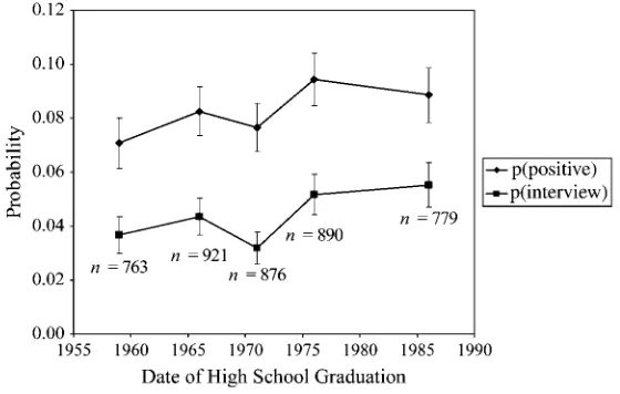
Figures 1 and 2 show an upward trend for theinterviewresponse based on date of high school graduation, as in Equation 1.13Although no two adjacent years are
sta-tistically significantly different at the 5 percent level, the results are suggestive. In Massachusetts, the interview results show a statistically significant difference at the 5 percent level between the oldest,hsgrad59, and youngest,hsgrad86.
The most significant results are found by breaking up age categories into ‘‘older/ younger’’ groups where older is defined to be age 50, 55, and 62, and younger is de-fined to be ages 35 and 45.14Table 1 describes t-test results comparing the mean
Figure 1
Response Rates in Massachusetts
Note: Vertical bars indicate standard errors.
13. Results for thepositiveresponse are included in charts and available on request, but this paper will focus oninterviewresults, which are stronger for the following reasons. First, not all ‘‘positive’’ responses may actually be positive—some asking for more information could be preludes to rejection, thus, producing measurement error. Secondly, more subtle forms of discrimination, such as calling one person back more enthusiastically than another, are less likely to be discovered than overtly failing to call back the older can-didate. In fact, the caller may not even realize that he or she has treated the candidates differently. 14. I also tried breaking up older and younger categories by placing 50 in the younger category (older2and
younger2) and leaving 50 out altogether (older3andyounger3). Results were similar across categories but de-fining 50 as older produced the strongest results. Additionally, there may be some worry about that the results are being driven by the ends of the distribution, ages 35 and 62. Although this would still be indicative of dif-ferential treatment by age, results are similar removing these age groups from the distribution. Coefficients for interview are identical at the second decimal place to those presented in Table 1 and significant at the 10 percent level with a two-tailedt-test and at the 5 percent level with 1-tail in Massachusetts and still significant at the 5 percent level for Florida.
response rates for these two age categories with and without controls. For interviews, there is a difference of 1.6 percentage points, or 42 percent, for Massachusetts and 2.0 percentage points, or 46 percent, for Florida.15The mean younger job seeker in Mas-sachusetts needs to file, on average, 19 applications to get oneinterviewrequest, while an older job seeker needs to file 27. In Florida, a younger worker needs to file 16 and an older worker 23 applications to get aninterviewresponse. A marginal probit including olderas an age dummy results in a negative and significant coefficient forolderfor interviews for both cities, as shown in Table 2, columns 6 and 12.
A final way of looking at the effect on age is to actually regress on age as if it were a continuous variable. This method provides more power than using age dummies. Columns 5 and 11 in Table 2 show that the coefficient on age given by the marginal effect of the probit is negative and significant at the 5 percent level for theinterview response, with each additional year of age causing a worker to be 0.08 percent less likely to be called back for an interview in Massachusetts and between 0.075 percent and 0.09 percent less likely to be called for an interview in Florida. Thus, there is differential interviewing by age. Assuming linearity,16for each additional ten years
of age the mean applicant would have to answer five additional ads in Massachusetts and 3.5 in Florida to receive an interview request.
Figure 2
Response Rates in Florida
Note: Vertical bars indicate standard errors.
15. If I take the lowest point in the confidence interval for younger workers and divide that by the highest point in the confidence interval for older workers, and then do the same with the highest point for younger workers and lowest point for older workers, I get a range of a younger worker being -0.05 to 113 percent more likely to get an interview in Massachusetts and -0.02 to 117 percent more likely to get an interview in Florida. 16. An age-squared term came up insignificant in probit regressions. However, I cannot reject a cubic age specification for the interview response in the Florida set. The cubic age specification is not significant in the Massachusetts set.
Table 1
Mean Response Rates by Age and State
Older Younger Difference Number of Ads Needed for One Response
Older Younger
Positive Interview Positive Interview Positive Interview Positive Interview Positive Interview
MA 0.077 0.038 0.092 0.053 0.015 0.016 12.99 26.67 10.91 18.75
[2560] [2560] [1669] [1669] (0.09) (0.01)
FL 0.091 0.043 0.108 0.062 0.017 0.020 10.98 23.42 9.30 16.07
[2295] [2295] [1478] [1478] (0.10) (0.01)
Notes: Older includes ages 50, 55, and 62 and younger includes ages 35 and 45. Cell number is reported in brackets.P-values are reported in parentheses and refer to two-tailedt-tests.
38
The
Journal
of
Human
Table 2
Marginal Effect of Age on Likelihood of a Response
Massachusetts Florida
Positive Interview Positive Interview
(1) (2) (3) (4) (5) (6) (7) (8) (9) (10) (11) (12)
age 20.00083 20.00080 20.00043 20.00075
(0.00041)* (0.00032)* (0.00046) (0.00035)*
older 20.016 20.017 20.015 20.018
(0.007)* (0.006)** (0.008)+ (0.007)*
hs59 20.022 20.018 20.002 20.010
(0.011)* (0.007)* (0.014) (0.009)
hs66 20.008 20.012 20.012 20.026
(0.012) (0.008) (0.013) (0.008)**
hs71 20.016 20.023 20.003 20.010
(0.010) (0.007)** (0.013) (0.008)
hs76 0.002 20.005 0.017 0.001
(0.012) (0.008) (0.014) (0.009)
Observations 4229 4229 4229 4229 4229 4229 3773 3773 3773 3755 3755 3755
Ho† 7.13 4.01 4.83 15.02 6.23 9.40 5.60 0.86 3.10 13.92 4.58 6.48
Ho: p-value (0.129) (0.045) (0.028) (0.005) (0.013) (0.002) (0.231) (0.353) (0.078) (0.008) (0.032) (0.011)
+ significant at 10 percent; * significant at 5 percent; ** significant at 1 percent Ho; † Age effects are all zero (fromF-stat)
Notes: Results reported are marginal effects from a probit equation using the margfx command in Stata. Robust standard errors in parentheses. Older includes ages 50, 55,
and 62 and younger includes ages 35 and 45. The hs dummies refer to the year of high school graduation listed on the resume. The dummyhs86is omitted. Controls
include years out of ten in the labor force, years out of ten in the labor force squared, workgap, college, computer classes since 1996, volunteering, sports, already has insurance, flexible, attendance award, typos, and the following occupational dummies: professional, education, health, manager, sales, craftsman, operative, service, and laborer. For the interview outcome, education and laborer predict failure perfectly and 18 and 133 observations are dropped respectively. Results are clustered on firm.
Lahey
Companies could also discriminate in more subtle ways than by failing to call back or to ask for an interview. Other possible outcomes are calling back the younger appli-cant sooner than the older appliappli-cant, or calling back the younger appliappli-cant multiple times but only calling the older applicant once. Although there are examples where ei-ther of these outcomes is the case, on average the evidence of discrimination is not sta-tistically significant for either of these possibilities (results not shown). I also examined actual negative responses, however not only were there very few of these, but I have reason to believe that when negative responses are sent out, many of them are sent via postal mail.17Because I do not have information on postal responses for the major-ity of applications, it is not feasible to use negative responses as an outcome.
B. Reasons for Differential Interviewing by Age
1. Statistical Discrimination
My experimental setup enables me to explore different possible reasons for this dif-ferential treatment, or discrimination.18The first type of discrimination I look at is
statistical discrimination, which, in its most basic definition, is judging an individual on group characteristics rather than individual characteristics. More formally, I uti-lize the model by Phelps (1972) as outlined in Aigner and Cain (1977), which assumes that employers measure expected skill through an indicator y based on the observed true skill levelqand a measurement erroru, thus,y¼q+u. I assume that the variance ofuis equal for the two groups and the variance ofqis greater for older workers than for younger.19Within this model, positive information about ability,
that is, a highery, helps older workers more than it helps younger workers (they-E(q) graph will have a steeper slope for older workers than for younger). For example, an indication that an older worker has taken a computer class will cause a greater marginal increment to expected productivity for the older than for the younger worker, that is, it will help an older worker more than it will help a younger worker.20
17. In the Massachusetts part of the sample, I was able to collect mail at one of the two addresses that were randomly assigned to resumes. Through this collection, I did not find anypositiveorinterviewresponses, but did receive some negative responses. The majority of written responses were post-cards stating receipt of the application. There were a few requesting more information, but these companies also requested more infor-mation via phone or email.
18. I do not differentiate between stereotypes that are true (and thus, fit in standard models of statistical discrim-ination, such as Phelps 1972) and stereotypes that are false, but that employers believe to be true. One can make the argument that because workers who are hired young often age into the firm, firms that employ larger numbers of workers may have some experience with older workers and are less likely to believe false stereotypes. Additionally, the notion of feedback effects (as in Lundberg and Startz 1983) into educational choices is less of an issue because even though older workers may choose training, the majority of education decisions have already been made. There may still be feedback effects in terms of decisions whether or not to remain in the labor market, however. 19. In this model, average true ability for the two groups is assumed to be either equal or lower for older workers than for younger. Recall that even though the Aigner and Cain (1977) model focuses on wage dif-ferentials, in fixed wage (for example, minimum wage or salary scale) jobs like the majority of those in this experiment, the hiring margin will adjust when the wage margin cannot.
20. Different assumptions provide a model where the test is less reliable for older workers and thus, a pos-itive ability signal would help younger workers more than older. However, there is no reason to assume that either younger workers have larger variance in, for example, computer ability or that they would get more out of a basic computer skills course than older workers, unlike the case where many black high schools are assumed to be of more variable or worse quality than many white high schools.
I tested for statistical discrimination by randomly including items on resumes that signaled that the worker did not fit into a standard stereotype.21For example, to test whether employers think older workers are inflexible and unchanging, I include a statement that the applicant was flexible or ‘‘willing to embrace change.’’ To test for the effect of these variables on the probability of getting a callback or interview, I interact each of these variables witholder:
pr½Responsei¼1 ¼F½B1ðControlsÞi+B2ðQiÞ+B3ðOlderiÞ
+B4ðOlderiQiÞ ð2Þ
whereQis the reason for statistical discrimination that is being tested andControls include the number of years of work history out of ten, typos, college experience, relevant computer experience, volunteer work, sport, other hobby, insurance, flexibil-ity, attendance award, and a set of occupation dummies, except when the reason tested is one of those controls. Detailed results for Equation 2, as well as for a fully interacted version, are available on request.
Employers may discriminate statistically because they fear that older workers will ‘‘cost’’ more in terms of absences and benefits.22To test whether or not companies discriminate statistically against older workers because they assume older workers will have more absences, I introduced an item on the resume saying that the applicant had won an attendance award. This variable is positive but not significant at the 5 percent level. If anything, attendance awards help younger workers more than older in terms of magnitude. To see whether or not higher health insurance costs are a rea-son older workers are not hired, I put in the statement that a worker does not need in-surance coverage.23Already having insurance increases the likelihood of getting an interview in Massachusetts, but helps only younger workers and may hurt older work-ers in Florida, although, again, these results are not statistically significant. Employwork-ers could also fear that older workers may be less likely to have reliable transportation, and thus, may be tardy or absent from work for this reason. There is no evidence that com-mute time, matched by zip code to place of work PUMA (public use metropolitan area) affects older or younger workers differently (results not shown).
21. Stereotypes examined came from a list of the top 10 reasons for discrimination against older workers according to a 1984 survey of 363 companies in which hiring managers were asked for reasons that other companies might discriminate against older workers (Rhine 1984). Not all top 10 reasons could be explored using this experimental design; those will be explored separately in future research. For example, Lahey (2006) finds strong negative hiring effects of age discrimination legislation on men, but not women. 22. As mentioned in the previous section, unless otherwise noted, this list of statistical discrimination items came from a survey by Rhine (1984), with the exception of transportation costs, which was suggested by a seminar participant. Rhine (1984) surveyed hiring managers in firms and asked them why they thought that other hiring managers might be less likely to hire older workers.
23. Although, according to Blue Cross/Blue Shield of Massachusetts (personal communication) and Sheiner (1999), health insurance costs vary less with age for women than for men (the possibility of preg-nancy goes down as a woman ages), there is some doubt that human resource managers are aware of the fact. Additionally, insurance costs may not follow the same pattern in all cases. Scott, Berger, and Garen (1995) find that older age hiring is lower in firms that offer health insurance and in firms where health in-surance is more expensive. However, firms that offer benefits such as health inin-surance are different than firms that do not. For example, they tend to be larger and have steeper earnings profiles as well (Idson and Oi 1999). Firms with different healthcare costs may also differ in ways not exogenous to employee age.
Employers may also worry that older workers will not be as productive as younger. First, they may believe that older workers’ knowledge and skills are obsolete. For this reason I added a variable indicating that the worker had gotten a computer cer-tificate in 1986 (which would be outdated), 1996, or 2002/2003, when such skills would be relevant and recent. While not significant, relevant computer experience helps younger workers more than older workers to get interviews in Florida. How-ever, in Massachusetts, it helps older workers more than younger, although the inter-action term is not significant.24Vocational training25 helps younger workers more than older workers to get interviews. An interaction between vocational training and older (not shown) is significant at the 5 percent level for Florida, but not for Mas-sachusetts. Second, employers may be worried that older workers lack energy. To test this reason, I introduced an item on the resume saying the applicant plays sports. For the most part, this variable is not significant. It is significant and positive at the 5 per-cent level for the interview response for younger workers and workers overall in Florida and negative but not significant for workers in Massachusetts. Interaction terms betweensportsandolderare not significant.
Third, previous research has suggested that older women use volunteer work as a ‘‘stepping stone’’ to labor market work (Stephan 1991), and, indeed, I find that hav-ing volunteer work listed helps older women more than younger.26Fourth, Bendick, Jackson, and Romero (1996) find that the biggest help to an older worker’s resume is to signal that he or she is flexible or ‘‘willing to embrace change.’’ Although the in-teraction term is only significant for Massachusetts, I found that having this state-ment on a resume hurts an older worker, but does not hurt a younger worker.27 This difference in findings may be because the AARP has been recommending that older workers put such statements on their resumes since the time of Bendick’s study and thus, this statement now signals that the worker is old.
Finally, experience may interact with age as a form of statistical discrimination. Employers may assume that older workers have more experience, or they may be prejudiced against an older worker if she does not have more experience than a youn-ger worker. I looked at this issue in two different ways. First, I looked at the effect of previous experience in the applied-for occupation for the different age groups. Al-though no interactions of same-occupation experience with age are significant at the 5 percent level (not shown), having occupational experience listed on the resume similar to the occupation being applied for helps younger workers more than older workers as shown in Table 3, Columns 1–6. However, a different effect is found for implied experience—that is, when the want-ad requires experience;28 older
24. Interaction results have also been done using the Norton adjustment, and the results still hold (Norton, Wang, and Ai 2004). Some magnitudes may change, but signs and 5 percent significance do not. 25. Note that occupation and vocational training are related mechanically in this experiment because voca-tional training was only included in resumes for which it was required (such as dental assisting or nursing). 26. The interaction of older and volunteer is positive and significant at the 20 percent level forpositive
outcomes and 30 percent level for interview outcomes in Florida, but only at the 40 percent level for in-terview in Massachusetts.
27. The interaction of older and flexible is significant at the 5 percent level for the interview variable in Massachusetts and at the 60 percent level for Florida.
28. Admissible want-ads could include requirements of up to a year of experience, whether the applicant had it on the resume or not.
Table 3
The Effect of Experience on Interview Requests
Massachusetts Florida Massachusetts Florida
All Older Younger All Older Younger All Older Younger All Older Younger
(1) (2) (3) (4) (5) (6) (7) (8) (9) (10) (11) (12)
same 0.018 0.013 0.024 0.016 0.004 0.037
experience (0.011) (0.012) (0.016) (0.012) (0.012) (0.019)
experience 20.023 20.019 20.028 20.031 20.029 20.036
required (0.008)** (0.008)* (0.011)** (0.009)** (0.009)** (0.013)**
Observations 3,651 2,207 1,444 3,266 1,980 1,168 4,228 2,560 1,668 3,755 2,267 1,427
* significant at 5 percent; ** significant at 1 percent
Notes: Results reported are marginal effects from a probit equation using the margfx command in Stata. Standard errors are reported in parentheses. Same experience refers to whether or not the resume had experience similar to that on the resume. Experience required refers to whether or not experience was required in the advertise-ment. Older includes ages 50, 55, and 62 and younger includes ages 35 and 45. Controls include years out of ten in labor force, years out of ten in labor force squared, workgap, college, computer classes since 1996, volunteering, sports, already has insurance, flexible, attendance award, typos, and the following occupational dummies: professional, education, health, manager, sales, craftsman, operative, service and laborer. Results are clustered on firm.
Lahey
workers were hurt less than were younger workers, as shown in Table 3, Columns 7-12, although again, this interaction is not significant at the 5 percent level. Thus, there is slight evidence that employers are more likely to give older workers the ben-efit of the doubt in terms of experience, but only when neither applicant lists the re-quired experience on the resume. Otherwise, having the rere-quired experience may help younger workers more than older. This possibility suggests that the entry-level labor market may be different in terms of age discrimination from markets requiring more experience.
2. Taste-Based Discrimination
Employers may also use taste-based discrimination, which is when a group of people, either employers, employees, or customers, have ‘‘tastes’’ for discrimination; that is, they prefer one group over another based on tastes rather than any economic rationale.
a. Employer
Employer taste-based discrimination would occur if employers (or those doing the hiring) preferred younger workers to older. Human resource profes-sionals may have less taste-based discrimination because of training and knowledge of discrimination laws, although they might be more likely to practice statistical dis-crimination based on learning from past hires. Bendick, Jackson, and Reinoso (1994) assume that firm size is a proxy for having a human resources department and finds that there is no link between race discrimination and firm size. I found no link be-tween having a human resources department and being more or less discriminatory.29 In my study, firms with human resources departments may be more likely to inter-view younger workers, which would support the case of statistical rather than taste-based discrimination, but this finding is not significant.30The controlled coef-ficient on the interaction term betweenOlderandHRfor Florida for theinterview outcome is -0.025 with a standard error of 0.026 and this coefficient for Massachu-setts is -0.030 with a standard error of 0.0214.
b. Employee
Another form of taste-based discrimination would occur when employ-ees prefer to work with younger rather than older workers. Younger employemploy-ees might have a stronger distaste for working with older people than older employees do, espe-cially when the older employee is in a subordinate position. To test for this type of dis-crimination, I match zip codes from my dataset to place of work PUMA information on
29. I also have a rough variable for firm size (fewer than 15 employees, 15–19 employees, 20 or more employees). I find no relationship between firm size and hiring practices.
30. Another possible way of measuring employer taste-based discrimination is to examine the interviewing interaction between the ages of employers or human resources professionals and applicants. However, I have been unable to collect information on employer age. In addition, just because an employer is a mem-ber of a group does not mean that he or she will not discriminate against other memmem-bers. For example, Dick Clark, age 76, has been sued for age discrimination http://www.cnn.com/2004/LAW/03/02/dick.clark. sued.ap/.
worker age from the Census and look at the effect of percentage of workers over 40, over 50 and over 61 employed in the PUMA.31I find no effect of the age of a company’s workforce on the differential interviewing by age, thus, providing no support for em-ployee taste-based discrimination (results not shown).32However, this measure may
be too crude, as it matches zip code to place of work PUMA information rather than using the percentage of workers by age in a firm.
c. Customer
A final source of taste-based discrimination comes from the con-sumer base. Concon-sumers may prefer to buy from or interact with employees who are like them, so this discrimination should be even higher in occupations where there is interaction with the public, such as in sales and service. To test for this type of discrimination, I used the census to get age profiles of zip codes in Florida and Massachusetts and matched them to the zip codes of the companies applied to in the study. There is no evidence of consumer taste-based discrimination; firms in areas with higher percentages of population over the age of 50 are more likely to call back or to interview in general, and these results are stronger for younger workers than for older. The results are similar when only service and sales positions are looked at (results not shown). Thus, there is no evidence that younger consumer bases prefer workers in the same age group.
IV. Conclusions
These differential responses have real implications for older potential workers. Aside from the psychological implications of implied rejection, there are economic consequences that are more severe for some occupations than others. First, the number of positions open and available each week is limited and varies by occu-pation. For example, on a randomly chosen Sunday in Florida, there were 34 LPN (licensed practical nurse) jobs being offered but only eight preschool teacher posi-tions. Some professions have even fewer openings. Second, the number of applica-tions sent to receive an interview varies by occupation. Using general occupation categories, the number of applications needed for an interview ranges from a low of 5.5 for younger workers and ten for older workers in healthcare positions in Flor-ida to a high of 32 ads for younger workers and 72 ads for older workers seeking clerical positions in Massachusetts.33Finally, given that the wages in many of these
31. This effect of older workers in a company influencing the age of new hires is not mechanical because older employees may have been hired young and aged with the company.
32. For the percentage older than 50 interaction withOlder, the Florida coefficient is 0.00139 with a stan-dard error of 0.00286 and the Masssachusetts coefficient is -0.660 with a stanstan-dard error of 0.478. 33. With ‘‘low’’ and ‘‘high,’’ I am only including general occupation categories that have at least 200 resumes sent. There are some occupational categories with low sample sizes, such as professional/technical nonhealthcare (mostly preschool teachers) in Florida that received no responses for older workers, and thus, would, by the metric used, require an infinite number of resumes to receive an interview. However, only 51 resumes were sent to p/t nonhealthcare positions in Florida. There were 558 healthcare resumes sent in Florida and 1,057 clerical resumes sent in Massachusetts.
occupations are not very high (often minimum wage), it is likely that persons seeking these jobs also do not have a large amount of wealth to finance an extended job search, especially if they are ineligible for unemployment benefits.
What does this mean for older vs. younger workers? Conditional on getting an in-terviewresponse, it takes, on average, eight days to be offered an interview. I have not been able to find information on the number of interviews it takes to get an entry-level job, but one online firm34finds that it takes seven to ten interviews on average for a college graduate to obtain a job offer. Using a back of the envelope calculation for one of the professions most likely to be hired, a new licensed practical nurse35 sending out 30 applications a week can expect three interviews a week as an older worker and six interviews a week as a younger worker. Assuming it takes seven to ten interviews to land a job, the average younger worker could expect an employ-ment offer in a little over a week, compared with three weeks for an average older worker. But this is the best-case scenario. An older worker attempting to find clerical work could file close to 100 applications per week and expect to be given an offer seven to ten weeks later (a younger worker would get an offer in half that time), us-ing the same back of the envelope calculation, and that assumes there are 100 unique new clerical ads each week, which is unlikely as a large number of ads are run at least two weeks in a row. For someone who needs to work because of a lack of sav-ings, several months without income could be critical.
This study clearly shows differential interviewing by age for entry-level positions in contemporary labor markets. I find that younger applicants are 42 percent more likely than are older applicants to be offered an interview in Massachusetts and 46 percent more likely in Florida. The extent of discrimination against older workers is similar to that of discrimination against women or blacks.36I found no evidence of taste-based discrimination. I found some suggestive evidence for statistical dis-crimination against workers along a few dimensions, such as skills obsolescence, as signaled by adding relevant computer experience to a resume (but only in Massa-chusetts). Many resume items helped younger workers but either hurt or did not af-fect older workers. Pinpointing the reasons for differential treatment by age is a fertile area for future research.
Additionally, future research needs to be done exploring other labor markets, such as the nonentry-level market. In nonentry-level positions, there may be taste-based discrimination against younger workers supervising older workers, which would sug-gest that there would be less age discrimination against older workers in these mar-kets. For example, managerial positions in Florida (but not Massachusetts) tended to prefer older workers, interviewing 4 percent of older applicants and 1 percent of
34. See website: www.onestop.com
35. A profession that takes 1 year of training and had a median salary of $31,440 in 2002 according to the BLSOccupational Outlook Handbook.http://bls.gov/oco/ocos102.htm
36. Neumark (1996) find evidence of 47 percent differential interview requests against female wait staff in high-price restaurants and 40 percent toward female wait staff in lower-price restaurants. Bertrand and Mullainathan (2004) find that applicants with white sounding names are 50 percent more likely to be called for an interview than applicants with black sounding names. It is somewhat difficult to compare the extent of the magnitude of age discrimination to race or gender discrimination, since age is not a binary variable and breaking into older and younger categories can be done arbitrarily. I might have found more had I been comparing, for example, 32-year-olds to 90-year-olds.
younger workers. I also found differences in differential interviewing between occu-pations; blue-collar and male-dominated occupations in the sample tend to prefer older workers to younger. Because these occupations in my sample tend to be clus-tered in dying industries, there may be a bias toward hiring workers with shorter expected future work-lives. (Sample sizes are not large enough to present these results in detail.)
This study provides evidence supporting the idea that the demand for labor from older workers is smaller than that for younger workers. Simply encouraging older workers to reenter the labor force may not guarantee that they will be able to find jobs in a timely manner, if at all. This study also has important implications for women who are most likely to need additional work—those with little work experi-ence who need to enter the labor market unexpectedly, such as widows, those whose husbands have lost jobs and cannot find employment, or divorcees. Although there are more older women than older men, the majority of economic surveys on aging and work focus on a random sample of men and, if they include women at all, only include spouses. Regardless of the reasons for differential treatment, any policy that depends on older people finding work to maintain their quality of living, such as changing Social Security benefits, needs to consider the demand side for their work.
Appendix 1
Data
The use of a computer program to randomly generate items in order to create many different possible resumes is a large improvement over earlier studies. First, unlike studies where a limited number of resumes are used, the use of many combinations lessens (and can test for) the possibility that an employer is reacting to something specific in the particular resume sent out. Moreover, because there is no human in-teraction with the resume during its creation, the possibility of injecting subjectivity into the process of matching resumes with job openings is completely eliminated. Resumes and resume items (other than the objective) are truly randomly assigned to job openings, eliminating many possibilities for bias.
The computer program used to prepare and match resumes is best explained through example. Say that a job vacancy for a receptionist has been found. The re-searcher will open the computer program specifying jobs for a receptionist position. The computer program will first randomly choose two of the possible women to ap-ply to the job, for example, Linda Jones (age 45) and Mary E. Smith (age 62). It will then pick an objective statement for Linda (‘‘To obtain a position as a receptionist’’) and a matching one for Mary (‘‘To secure a position as receptionist’’). Similarly it will match work histories and high school. Next it will decide whether or not to test for one or more of the possible reasons for discrimination through adding items to the resume. As an example, to see if lack of energy is a reason employers discriminate against older people, the computer will put under hobbies that Linda Jones is a tennis player, then designate Mary E. Smith as a racquetball player. Regressions found no significant difference between response rates for tennis and racquetball players, or any of the other possible paired choices.
Variations on the resumes ranged as follows. Candidates were named Mary E. Smith or Linda Jones.37 The objectives included sales positions, office positions, entry-level nursing positions, wait staff positions and other entry-level or close to entry-level positions that require only a year of combined post-high school education and experience to obtain. All resumes had the applicant currently working at a job. Dates of high school graduation included 1959, 1966, 1971, 1976 and 1986. High schools chosen were Ames High School in Ames City, Iowa and DeKalb High School in DeKalb, Illinois. Some resumes listed experience in computer classes, either from 1986, which makes such experience obsolete, 1996, when the experience is useful but not recent, or 2002/2003, when the experience is both useful and recent. Current employment varied as well and ranged from cashier work to secretarial work with a couple of ‘‘unusual’’ jobs possible, such as those giving fork-lift experience. Volunteer work included work at homeless shelters or food banks. Hobbies included some combination of tennis, racquetball, gardening and crafting. An attendance award could also be listed. All resumes had email addresses listed.38Appendix Tables A1a and A1b show how resume characteristics were distributed across high school graduation dates.
Typos were introduced to the study in two different ways: First, purposeful typo-graphical errors were programmed into the resume machine during the first half of the study when there was more interviewing in general. These typos were represen-tative of those found in actual resumes—they included things like missing punctua-tion marks, large words that had been misspelled and inconsistent indentapunctua-tion. The second kind of error was introduced inadvertently when applying for a job that did not fit one of the major job categories in the resume program. These errors in-cluded things like putting an ‘‘a’’ where an ‘‘an’’ should be or other similar mistakes that native English speakers do not often make. There are many fewer of these errors and they tend to be most prevalent in Florida and when there was a research assistant regime change.
Forty want-ads were drawn without replacement per week per city from the Sunday Boston Globe and the online version of the St. Petersburg Times. For the Boston Globe, the number of pages of nonprofessional want-ads was counted. Then this number was entered into a random number generator to pick a random page. On this page, the number of want-ads on the page were counted. This new number was entered into a random number generator. That number ad was circled and checked to see if it: (1). advertised an entry-level job, (2). provided a fax or phone, or email address, and (3). had not been applied to in a previous week. If it did not fit those criteria, another ad from the same page was chosen. If it did fit those criteria,
37. Mary gets a middle initial because in my experience, and the experience of those with whom I have spo-ken, anyone over the age of 30 whose first name is Mary always adds her middle name or middle initial, es-pecially if her last name is also common (unless there’s a ‘‘Peter, Paul, and.’’ in front of the Mary). I have not had the same experience with Linda as a first name, although when asked, Linda’s middle initial is M. 38. The census finds that 47 percent of householders age 45 to 64 have internet access at home (http:// www.census.gov/prod/2001pubs/p23-207.pdf). Additionally, places that help people find work, such as Pro-ject Able, strongly encourage applicants to get email addresses and many job finding sites actually take seekers through the steps of signing up for a free hotmail account. Finally, adding an email address to an older resume is likely to work in the older resume’s favor, and thus, I should find even lower acceptance rates for older workers without adding email addresses.
Table A1a
Summary Statistics: Massachusetts
Variables All Older Younger 1959 1966 1971 1976 1986
Resume characteristics
hsgrad 1971.561 1965.625 1980.667 1959.000 1966.000 1971.000 1976.000 1986.000 yrs of 10 in LF 5.590 5.567 5.624 5.468 5.692 5.522 5.697 5.542
typo 0.163 0.171 0.151 0.118 0.198 0.188 0.181 0.117
college 0.196 0.195 0.197 0.204 0.203 0.177 0.212 0.180 computer 0.520 0.523 0.515 0.512 0.533 0.522 0.509 0.521 volunteer 0.504 0.498 0.513 0.509 0.481 0.508 0.520 0.506 sport 0.487 0.483 0.494 0.481 0.493 0.474 0.494 0.493 other hobby 0.196 0.192 0.202 0.210 0.186 0.183 0.199 0.205 insurance 0.503 0.508 0.496 0.528 0.506 0.493 0.487 0.506 flexible 0.517 0.523 0.508 0.533 0.511 0.525 0.515 0.501 attendance 0.493 0.500 0.482 0.499 0.489 0.513 0.480 0.485 recent computer 0.152 0.151 0.154 0.168 0.145 0.142 0.139 0.171 relevant computer 0.378 0.377 0.379 0.377 0.381 0.373 0.376 0.383
age 49.439 55.375 40.333 62 55 50 45 35
Method of sending
fax 0.786 0.780 0.795 0.790 0.771 0.780 0.816 0.772
email 0.179 0.186 0.170 0.176 0.191 0.188 0.157 0.185 online 0.034 0.034 0.034 0.033 0.037 0.032 0.027 0.041 Firm characteristics
EOE/AA 0.124 0.127 0.119 0.127 0.135 0.120 0.110 0.130 professional 0.040 0.039 0.040 0.045 0.043 0.031 0.042 0.039 education 0.025 0.028 0.020 0.022 0.033 0.027 0.020 0.021 (continued)
Lahey
Table A1a(continued)
Variables All Older Younger 1959 1966 1971 1976 1986
health 0.140 0.146 0.132 0.144 0.147 0.146 0.145 0.118 manager 0.066 0.062 0.070 0.072 0.054 0.062 0.064 0.076 clerical 0.250 0.252 0.247 0.249 0.256 0.250 0.230 0.266 sales 0.245 0.245 0.244 0.241 0.254 0.240 0.240 0.248 craftsman 0.022 0.021 0.024 0.024 0.017 0.023 0.022 0.026 operative 0.044 0.043 0.046 0.045 0.048 0.037 0.049 0.041 service 0.145 0.140 0.154 0.135 0.126 0.159 0.162 0.145 laborer 0.018 0.019 0.017 0.017 0.015 0.025 0.018 0.017
# observations 4,229 2,560 1,669 763 921 876 890 779
Notes:
hs grad age hs grad age
Older includes: hs1959 62 Younger includes: hs1976 45
hs1966 55 hs1986 35
hs1971 50
50
The
Journal
of
Human
Table A1b
Summary Statistics: Florida
Variables All Older Younger 1959 1966 1971 1976 1986
Resume characteristics
hsgrad 1971.538 1965.654 1980.675 1959 1966 1971 1976 1986 yrs of 10 in LF 5.694 5.674 5.726 5.684 5.672 5.667 5.752 5.696
typo 0.259 0.264 0.252 0.206 0.282 0.296 0.288 0.211
college 0.186 0.190 0.179 0.183 0.207 0.180 0.159 0.201 computer 0.511 0.506 0.518 0.506 0.501 0.510 0.522 0.514 volunteer 0.494 0.494 0.493 0.523 0.478 0.484 0.484 0.502 sport 0.499 0.493 0.508 0.495 0.508 0.478 0.513 0.502 other hobby 0.183 0.179 0.188 0.189 0.177 0.173 0.188 0.188 insurance 0.500 0.505 0.493 0.536 0.484 0.496 0.484 0.502 flexible 0.510 0.515 0.502 0.513 0.495 0.536 0.511 0.492 attendance 0.500 0.496 0.505 0.508 0.499 0.483 0.526 0.482 recent computer 0.156 0.152 0.163 0.150 0.151 0.153 0.159 0.168 relevant computer 0.380 0.371 0.393 0.360 0.378 0.373 0.402 0.384
age 49.462 55.346 40.325 62 55 50 45 35
Method of sending
fax 0.837 0.839 0.834 0.831 0.839 0.847 0.830 0.838
email 0.134 0.136 0.129 0.145 0.134 0.132 0.137 0.120 online 0.029 0.024 0.037 0.024 0.028 0.022 0.033 0.042 Firm characteristics
EOE/AA 0.149 0.144 0.158 0.152 0.146 0.135 0.146 0.172 professional 0.008 0.007 0.009 0.007 0.005 0.008 0.008 0.010 education 0.005 0.005 0.004 0.004 0.005 0.006 0.005 0.003 (continued)
Lahey
Table A1b(continued)
Variables All Older Younger 1959 1966 1971 1976 1986
health 0.148 0.150 0.144 0.142 0.165 0.144 0.140 0.149 manager 0.048 0.044 0.053 0.051 0.035 0.047 0.058 0.048 clerical 0.262 0.264 0.260 0.247 0.280 0.263 0.263 0.258 sales 0.195 0.189 0.205 0.204 0.180 0.185 0.187 0.226 craftsman 0.042 0.042 0.041 0.043 0.038 0.046 0.044 0.038 operative 0.081 0.081 0.079 0.078 0.085 0.081 0.097 0.059 service 0.173 0.176 0.169 0.180 0.161 0.185 0.165 0.174 laborer 0.035 0.038 0.030 0.044 0.041 0.031 0.029 0.032
# observations 3,773 2,295 1,478 705 762 828 787 691
52
The
Journal
of
Human
it was copied to a word document for resume creation purposes later and a new page was picked randomly. For the St. Petersburg Times, a fixed number of want-ads appeared on each online page, otherwise the procedure was the same as for Boston. After 40 new ads were collected, resume creation and sending could begin. This procedure biases toward ads that ran multiple weeks or that, in Boston, had larger ads or shared pages with larger ads. Real job applicants may also share these biases.
Call-ins were performed because many entry-level jobs are never advertised via want-ad. I could not use walk-ins because a pilot study showed that, not only were walk-ins time consuming, but many of them generated actual paper job applications with questions whose answers were difficult to control, but hurt an application if left blank, for example, ‘‘Describe your ideal job situation.’’ In addition, there was a worry that a manager would connect the person picking up or turning in an applica-tion with the job applicant, rather than looking at the resume characteristics alone. To generate a call-in, a young woman randomly generated an entry in the telephone book. Because large firms tend to have more entries in the telephone book than do small firms, and certain industries, such as law offices, tend to have multiple entries, call-ins tend to have a slight bias toward generating these firms. However, they do a better job of generating small firms than do want-ads. The company was then called and asked, ‘‘Hello, my name is Elizabeth Williams, I was wondering, do you have any entry-level jobs available?’’ If the person on the phone did not understand, the caller followed with, ‘‘Are you hiring for any entry-level positions?’’ If the person on the phone said no, the caller moved on to another phone book entry. If the person on the phone said yes, the caller tried to elicit a fax number or email address and later generated a resume and sent it. If there was no fax or email available, the caller first checked to see if there was an online application, and if there was, she sent a resume via that method. Otherwise, the caller coded the company as ‘‘no fax/email avail-able’’ and generated another telephone book entry.
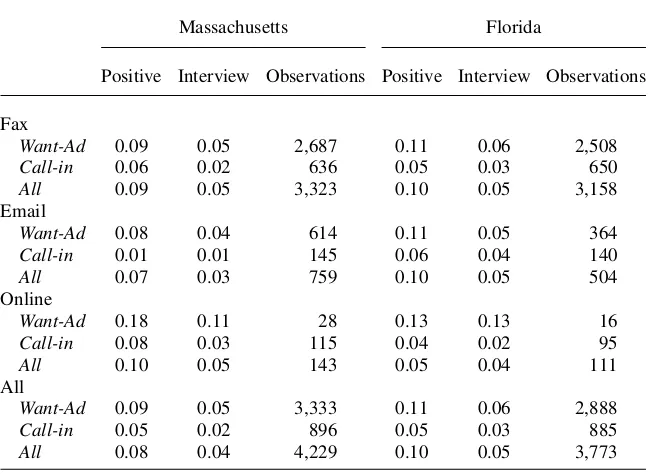
Response rates differ somewhat by method of application as shown in Appendix Table A2a. Want-ads are more likely to get interview responses than Call-ins, faxes slightly more likely than emails. There are some occupational differences in response rates between Massachusetts and Florida. For example, profes-sional/technical non healthcare positions, which are mostly preschool teaching positions, were 1.5 times as likely to hire younger workers in Massachusetts, but there was a much smaller number of positions advertised in Florida, so the sample size could not be compared. There was no difference in age for interview-ing healthcare workers, mostly Licensed Nurse Practitioners and Certified Nurse Assistants, in Massachusetts, but Florida healthcare agencies were twice as likely to hire younger workers (results not shown). The composition of jobs available differs as well, as can be seen under ‘‘firm characteristics’’ in Appendix Tables A1a and A1b. A quarter of the jobs available in both metropolitan areas were cler-ical work, but the Boston area was much more likely to hire sales workers, at 24.5 percent of openings compared to 19.5 percent in the St. Petersburg-Tampa area. Entry-level professional, education and managerial jobs were also more likely to be advertised in Massachusetts whereas craftsman, operative, service and la-borer jobs were more likely to be advertised in Florida. The order in which the resumes were sent did not matter.
Table A2b
Marginal Effect of EOE on Response Rate for Massachusetts
All Occupations Nonhealth Occupations
Variables Positive Interview Positive Interview
EOE/AA 0.025 0.016 20.001 20.002
(0.022) (0.016) (0.021) (0.014)
Older 20.015 20.018 20.015 20.017
(0.010) (0.007)* (0.009) (0.007)*
EOE/AA*older 0.000 0.012 20.009 0.004
(0.025) (0.020) (0.025) (0.021)
Observations 4,229 4,229 3,635 3,635
*significant at 5 percent
Notes: EOE refers to equal opportunity employment, and AA refers to affirmative action mentioned in the ad. Standard errors in parentheses. Results are from a marginal probit and standard errors are clustered on firm.
Table A2a
Response Percentage by Method of Delivery
Massachusetts Florida
Positive Interview Observations Positive Interview Observations
Fax
Want-Ad 0.09 0.05 2,687 0.11 0.06 2,508
Call-in 0.06 0.02 636 0.05 0.03 650
All 0.09 0.05 3,323 0.10 0.05 3,158
Want-Ad 0.08 0.04 614 0.11 0.05 364
Call-in 0.01 0.01 145 0.06 0.04 140
All 0.07 0.03 759 0.10 0.05 504
Online
Want-Ad 0.18 0.11 28 0.13 0.13 16
Call-in 0.08 0.03 115 0.04 0.02 95
All 0.10 0.05 143 0.05 0.04 111
All
Want-Ad 0.09 0.05 3,333 0.11 0.06 2,888
Call-in 0.05 0.02 896 0.05 0.03 885
All 0.08 0.04 4,229 0.10 0.05 3,773
References
Aigner, Dennis J., and Glen G. Cain. 1977. ‘‘Statistical Theories of Discrimination in Labor Markets.’’Industrial and Labor Relations Review30(2):175–87.
Arrow, Kenneth J. 1972. ‘‘Some Mathematical Models of Race Discrimination in the Labor Market.’’ InRacial Discrimination in Economic Life,ed. Anthony H. Pascal, 187–204. Lexington, Mass.: D.C. Heath.
Baltes, Paul B., Hayne W. Reese, and John R. Nesselroade. 1988.Introduction to Research Methods: Life-span Developmental Psychology.Hillsdale, N.J.: Lawrence Erlbaum Associates.
Becker, Gary S. 1971.The Economics of Discrimination.Chicago: University of Chicago Press.
Bendick, Marc, Lauren E. Brown, and Kennington Wall. 1999. ‘‘No Foot in the Door: An Experimental Study of Employment Discrimination Against Older Workers.’’Journal of Aging & Social Policy10(4):5–23.
Bendick, Marc Jr., Charles W. Jackson, and J. Horacio Romero. 1996. ‘‘Employment Discrimination Against Older Workers: An Experimental Study of Hiring Practices.’’ Journal of Aging & Social Policy8(4):25–46.
Bendick, Marc, Jr., Charles W. Jackson, and Victor A. Reinoso. 1994. ‘‘Measuring Employment Discrimination through Controlled Experiments.’’Review of Black Political Economy23(1):25–48.
Bernheim, B. Douglas. 1997. ‘‘The Adequacy of Personal Retirement Saving: Issues and Options.’’ InFacing the Age Wave, ed. David Wise. Stanford: Hoover Institute Press. Bertrand, Marianne, and Sendhil Mullainathan. 2004. ‘‘Are Emily and Greg More
Employable Than Lakisha and Jamal?’’American Economic Review94(4):991–1013. Burtless, Gary, and Joseph F. Quinn. 2001. ‘‘Retirement Trends and Policies to Encourage
Work Among Older Americans.’’ InEnsuring Health and Income Security for an Aging Workforce, ed. P. Budetti, R. Burkhauser, J. Gregory and A. Hunt, 375-415. Kalamazoo: The W. E. Upjohn Institute for Employment Research.
———. 2002. ‘‘Is Working Longer the Answer for an Aging Workforce?’’Boston College Center for Retirement Research Issue Brief11:1–12.
Diamond, Peter A., and Jerry. A. Hausman. 1984. ‘‘The Retirement and Unemployment Behavior of Older Men.’’ InStudies in Social Economics,ed. H. J. Aaron. Washington, D.C.: Brookings Institution.
Diamond, Peter and Peter. R. Orszag. 2002. ‘‘An Assessment of the Proposals of the President’s Commission to Strengthen Social Security.’’Contributions to Economic Analysis and Policy1(1).
Favreault, Melissa M., and Frank J. Sammartino. 2002.The Impact of Social Security Reform on Low-Income and Older Women.Washington, D.C.: Public Policy Institute.
Fix, Michael, George C. Galster, and Raymond J. Struyk. 1993. ‘‘An Overview of Auditing for Discrimination.’’ InClear and convincing evidence: Measurement of Discrimination in America., ed. Michael. Fix and Raymond. J. Struyk. Washington, D.C.: Urban Institute Press; distributed by University Press of America Lanham Md.
Hirsch, Barry T., David A. Macpherson, and Melissa A. Hardy. 2000. ‘‘Occupational Age Structure and Access for Older Workers.’’Industrial and Labor Relations Review 53(3):401–18.
Holden, Karen C., and Kathleen D. Zick. 1998. ‘‘The Roles of Social Insurance, Private Pensions, and Earnings in Explaining the Economic Vulnerability of Widowed Women in the United States.’’International Studies on Social Security.F. f. I. S. o. S. Security, Ashgate. 4. Holzer, H. J. 1996.What Employers Want: Job Prospects for Less-Educated Workers.New
York, Russell Sage Foundation.