T H E J O U R N A L O F H U M A N R E S O U R C E S • 46 • 2
The Effect of Random Income Shocks on
Marriage and Divorce
Scott Hankins
Mark Hoekstra
A B S T R A C T
Economists have long been interested in the extent to which economic re-sources affect decisions to marry and divorce. However, this issue has been difficult to address empirically due to a lack of exogenous income shocks. We overcome this problem by exploiting the randomness of the Florida Lottery and comparing recipients of large prizes to those of small prizes. Results indicate that while positive income shocks of $25,000 to $50,000 do not cause statistically significant or economically meaningful changes in divorce rates, single women are less likely to marry as a result of the additional income.
I. Introduction
Economists and other social scientists have devoted significant effort toward determining the relationship between economic resources and marital deci-sions. Interest began with work by Becker (1981) on how income affects an indi-vidual’s incentives to marry or divorce. More recently, researchers and policymakers have tried to determine whether income supports or tax credits for low-income households cause individuals to divorce or fail to marry, which many policymakers
Mark Hoekstra is an assistant professor of economics at the University of Pittsburgh, 4714 Posvar Hall, 230 S. Bouquet St., Pittsburgh, PA 15260. Scott Hankins is an assistant professor in the College of Pub-lic Health at the University of Kentucky, 121 Washington Ave., Suite 101, Lexington, KY 40536–0003. The authors would like to thank the Florida Lottery for providing them with the data on lottery winners. They also would like to thank Scott Carrell, Betsey Stevenson, Randy Walsh, two anonymous referees, and seminar participants at Vanderbilt University, the 2007 Meeting of the Southern Economic Associa-tion, and the 2008 Meeting of the Society of Labor Economists for helpful comments and suggestions. The usual disclaimers apply. The data used in this article can be obtained beginning six months after publication through three years hence from Scott Hankins in the College of Public Health at the Univer-sity of Kentucky at scott.hankins@uky.edu.
[Submitted November 2009; accepted June 2010]
would regard as an unintended consequence (Bitler, Gelbach, Hoynes, and Zavodny 2004; Cain and Wissoker 1990; Groeneveld, Tuma, and Hanan 1980; Hu 2003).
There are several reasons why positive income shocks could affect marital deci-sions. For married couples, more generous cash transfers may have a stabilization effect and relax financial constraints and arguments that lead to divorce. Indeed, the income shocks received by individuals in this study—$25,000 to $50,000—are suf-ficiently large to pay off the majority of the unsecured debt ($49,000) owed by the those on the brink of bankruptcy (Hankins, Hoekstra, and Skiba 2010).
On the other hand, increased resources may enable unhappy couples to incur the costs associated with divorce.1Schramm (2006) estimates that legal fees incurred
during divorce average $7,000 while the additional housing cost averages just over $4,000 per year.2 The short-term costs associated with divorce may be especially
important to the extent couples are liquidity-constrained or behave as such due to risk-aversion. Evidence consistent with widespread liquidity constraints is reported by Laibson, Repetto, and Tobacman (2001), who report that at least 63 percent of U.S. households pay interest on credit card debt every month. In addition, other studies have shown how individuals do not smooth consumption as predicted by the permanent income hypothesis (Shapiro 2005; Stephens 2003). Finally, even the seemingly long-term costs of divorce such as the increased cost of supporting two households are more temporary than one might expect; Kreider (2006) reports that 50 percent of individuals who divorce remarry within five years, and some who do not likely cohabit.
The theoretical effect of positive income shocks on marriage rates is also ambig-uous. While simple economic models of marriage predict that an increase in re-sources will make single individuals more attractive as marriage partners, it also makes single life more attractive (Burstein 2007; Moffitt 1992). In addition, more resources may facilitate marriage due to sociocultural ideals for weddings or married life that require greater assets (Edin 2000).
However, empirically determining whether economic resources affect marriage and divorce has been difficult due to a lack of exogenous pure income shocks. To overcome that identification problem, we exploit random variation in the magnitude of cash prizes won in the Florida Lottery.3The crucial identifying assumption is that
conditional on winning more than $600 (the threshold at which the names of the winners are recorded) for the first time, the amount won is random. Tests support this identifying assumption: winners of $25,000 to $50,000 come from similar
neigh-1. This theory has been popularized in the press. In an article entitled “Buy Low, Divorce High” published in theNew York Timeson August 12, 2007, one divorcee and beneficiary of the appreciation in the housing market is quoted as stating “Money is freedom. . . . We made enough money to be able to get divorced and support two households.”
2. Both the legal and housing cost estimates are for married couples with children; we were unable to document any other estimates of the average legal and housing costs associated with divorce. The estimate from Schramm (2006) on housing costs comes from Census reports on average housing costs reported for unmarried individuals. Consequently, it may understate the additional cost in the first year since moving to less expensive housing takes time and since the estimate ignores the actual moving costs.
borhoods as those who win less than $1,000, and perhaps more importantly, winners of large sums were no more or less likely to marry or divorcebeforewinning the lottery than were (future) winners of small sums.
Results indicate that large income shocks significantly reduce the likelihood that single women marry. Specifically, we find that single women are six percentage points less likely to marry in the three years following the positive income shock, which represents a 40 percent decline. This suggests that additional income may remove some incentive for single women to marry, at least over the short-term.
In contrast, large cash transfers do not affect the marriage rates of men or induce couples to divorce. We find that the divorce rate of married recipients of $25,000 to $50,000 in the three years following the income shock is between one-half and one percentage point lower than that of recipients of $1,000, which is small both in absolute terms and relative to the baseline three-year divorce rate of 8.5 percent. Estimates also allow us to rule out large absolute positive net effects of income shocks on divorce rates: even the upper bound of the 95 percent confidence interval implies that fewer than one in 70 married couples will divorce due to the positive income shock of $25,000 to $50,000.
II. Previous Literature
In assessing the role of economic factors in marital decisions, this study joins a significant existing literature. Perhaps the most closely related research is that which examines the impact of men’s or women’s earnings on divorce (for example, Hoffman and Duncan 1995; Weiss and Willis 1997).4However, by design
these estimates pick up the effect of income as well as reduced returns to speciali-zation. Furthermore, as Johnson and Skinner (1986) point out, it is hard to determine whether, for example, women work more hours in response to a higher expected probability of divorce, or whether women are more likely to divorce because they earn higher incomes. Similarly, it is difficult to believe that men in typical data sets who later receive positive income shocks did so randomly rather than because of personal qualities such as loyalty or interpersonal skills. This is problematic given that these characteristics could themselves yield stronger marriages, but are not ob-served by the econometrician. Finally, while perhaps the most promising variation in income came from the randomization of income guarantees in the Negative In-come Tax experiments, methodological problems and the complexity of the exper-iments have made it difficult to determine what aspect of the experexper-iments, if any, affected marital decision-making (for example, Groenveld et al. 1980; Cain and Wissoker 1990).
There is also a literature that examines the impact of income-changing life events on marital decisions. Bitler et al. (2004) and Hu (2003) found that reducing welfare benefits increases the likelihood of divorce, though given the nature of the policy it is impossible to distinguish the effect of the negative income shock from that of the
increased work requirement. In addition, while Charles and Stephens (2004) report that job displacement results in higher divorce rates, they argue that it is the infor-mation conveyed by the job loss that causes the divorce rather than the loss of income. This highlights the difficulty in determining the effect of incomeper seon marital stability in the absence of truly exogenous shocks to income.
III. Data and Identification Strategy
To identify the effect of income shocks on marriage and divorce, we exploit the variation in income that is caused by the size of lottery prizes in Florida. Specifically, we obtained data on winners from two games: Florida Lotto and Fantasy 5. Florida Lotto allows players to choose six numbers or have the computer select a number for them, while Fantasy 5 is similar except that there are only five numbers. Both games are parimutuel games in which the amount won is determined by how many numbers the winner matched, the total amount spent on that drawing, and how many players won. For example, while very few Florida Lotto players matched six of six numbers and won the average prize of $6 million, players who matched five of six numbers won an average of $4,200, though the prizes from some drawings were much larger.
Similarly, in Fantasy 5, players who matched five of five numbers prior to 2001 won an average of $20,000, though again the actual amount varied widely depending on how many players won relative to how many played. After 2001, players who matched five of five numbers won an average of $120,000, while players who matched four of five numberswhen no one matched five numberswon an average of $900. Finally, while it is possible for individuals to play up to ten times on each card, an analysis of Fantasy 5 winners revealed that no winners had played the same five numbers multiple times on the same card. As a result, although some people are more likely to enter our data than others (that is, those who play more frequently or who play multiple times on a card), conditional on winning $600 the amount won is unaffected by the number of plays paid for on a given card. Rather, the identifi-cation strategy that we employ largely relies on the assumption that conditional on matching five of six numbers (Florida Lotto) or five of five numbers (Fantasy 5) for the first time, one’s underlying propensity to marry or divorce is uncorrelated with how many winners there were relative to the number of players. As discussed later, an important advantage of this research design is that it is testable.
The data for the analysis of divorce include every lottery winner in Miami-Dade and Palm Beach counties from 1988 through 2004, during which there were 73,714 individuals who won up to $50,000, while the data for the marriage analysis include only Miami-Dade County winners.5These winners represent everyone who won at
least $600 by playing either Florida Lotto or Fantasy 5,6the minimum amount for
which records were kept. For each lottery winner, we observe the individual’s name
5. The data set for the analysis of marriage is smaller because we could not access electronic marriage records for Palm Beach County.
and home zip code, the amount won (adjusted for inflation), the date of the drawing, and the lottery game played. Finally, we note that while we do not observe the marital status of lottery players at the time of winning, this will not be a problem so long as the magnitude of the cash prize is determined randomly. That is, there should be no more unmarried recipients of large cash prizes than there are of small cash prizes.7 However, as discussed later, the fact that not all lottery winners are
married or single does change the interpretation of the marriage and divorce rates observed as well as the estimated impacts of winning $25,000 to $50,000.
Data on marriage and divorce come from public records in Miami-Dade and Palm Beach counties in Florida, which is an equitable distribution state with respect to the division of marital assets.8These data were linked to the lottery winner data on
the basis of first and last name and county of residence. However, before doing so, efforts were made to reduce the number of false positive matches made due to common names. Toward that end, we excluded all names that appeared more than once in the 2007 county phone records. In addition, if lottery records indicated that an individual with a unique name from a given county won more than once, we then use only the first time that individual won.9Importantly, this also means that
our identifying assumption is that conditional on winning more than $600 for the first time, the amount won is random. We emphasize this because although whether an individual ever wins a large prize clearly depends on frequency of play, the magnitude of thefirstprize won does not.
As shown in Tables A1 and A2 in the appendix, eliminating individuals with common names leaves 40,198 lottery winners for the divorce analysis and 26,629 winners for the marriage analysis. As shown in Table A1, restricting the sample in this way does not change the overall distribution of large and small winners, con-sistent with what one would expect from excluding common names. Moreover, we later test that this sample restriction does not undermine internal validity by showing the similarity in both the neighborhood characteristics and pre-winning marriage and divorce rates of large and small winners.
The remaining individuals reflect a frequency-of-play-weighted population of lot-tery players in South Florida who have relatively uncommon names, the latter of which likely means our sample underweights Hispanics in South Florida. Still, com-paring the neighborhood characteristics of our sample to the United States indicates that our sample is more Hispanic (42 versus 15.4 percent) and somewhat more Black (19 versus 13 percent) than the United States overall.10The neighborhood family
income of our sample is somewhat lower than that of Miami-Dade and Palm Beach counties ($40,400 versus $44,800), which in turn is lower than all of the United
7. To the extent that income shocks affect marriage or divorce decisions in the short term, this may not be true in the longer term. For example, if positive cash shocks induce married couples to divorce, we may well expect higher marriage rates (per lottery player) for that group in the longer term as individuals remarry. However, since we only examine divorce rates up to three years afterward and find no effect, we are less concerned that our marriage estimates would be biased.
8. This means that in the absence of other considerations (for example, children), a prize received by one spouse should be split equally. Consistent with this law, we find little differences in the effects based on whether the recipient was male or female.
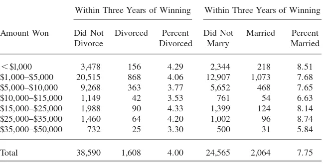
Table 1
Lottery Winners Linked to Marriage and Divorce Records after Winning
Within Three Years of Winning Within Three Years of Winning
Amount Won Did Not
⬍$l,000 3,478 156 4.29 2,344 218 8.51 $1,000–$5,000 20,515 868 4.06 12,907 1,073 7.68 $5,000–$10,000 9,268 363 3.77 5,652 468 7.65 $10,000–$15,000 1,149 42 3.53 761 54 6.63 $15,000–$25,000 1,988 90 4.33 1,399 124 8.14 $25,000–$35,000 1,460 64 4.20 1,002 96 8.74 $35,000–$50,000 732 25 3.30 500 31 5.84
Total 38,590 1,608 4.00 24,565 2,064 7.75
States ($50,000).11 We note, however, that since we do observe individual-level
income, we cannot rule out the possibility that the incomes of individuals in our sample are systematically above or below the average for their neighborhood.
Other evidence on the composition of lottery players comes from two sources. Clotfelter, Cook, Edell, and Moore (1999) analyze data from a nationally represen-tative sample of 2,400 adults and report that frequent lottery players are more likely to have lower incomes and less education than less frequent players. Kearney (2005) reports that while frequency of play is approximately equal across the income dis-tribution, college-educated individuals play approximately 40 percent less than high school graduates. In light of these studies and our own data, our judgment is that individuals in our sample are less well educated and likely have lower incomes than the average American. Thus, our findings are most likely to lead to externally valid predictions of the effect of pure income shocks on populations that are less well educated and somewhat poorer than the U.S. average.
The lottery winners in our sample were linked to divorce and marriage records filed in their respective county in the three years prior to and the three years after winning.12This was performed via an automated search of each winner’s first and
last name on the Miami-Dade County and Palm Beach County Clerk of the Court websites.
The results are shown in Table 1. Of the 40,198 winners, 1,608 (4.00 percent) were linked to a divorce case within three years after winning the lottery. For the marriage analysis, 7.75 percent of recipients were linked to a marriage license in the three years after winning.
While it is possible that some type I13and type II errors were made in linking
the lottery winners to divorce and marriage filings, neither type of error should invalidate the research design due to the randomness of amount won. That is, we should be no more or less likely to match winners of large jackpots to divorce or marriage records than we are to match winners of small jackpots, except for the causal effect of the income shock on marital decisions. Consequently, any difference in the marriage or divorce rates of small winners and large winners is properly interpreted as the causal effect of receiving a large cash prize.
One way to check our matching algorithm is to compare the divorce rates implied by our data to those from the Census. To do so, it is important to note that not all of the lottery winners are married. While we know of no measure capturing the proportion of lottery players or winners who are married, Clotfelter et al. (1999) report that lottery participation rates are approximately equal across divorced, mar-ried, and unmarried individuals.14A back-of-the-envelope calculation based on that
result and the demographic characteristics of residents of Miami-Dade and Palm Beach counties suggest that approximately 54 percent of the individuals in our data were married at the time they won the lottery.15Consequently, the annual divorce
rate as a proportion of married individuals who received less than $1,000 is (1.43/ 0.54) 2.65 percent per year. By comparison, 2.35 percent of married Floridians divorced in 2000 according to Census statistics.
An important advantage of our research design is that we can test the identifying assumption that the amount won is uncorrelated with the underlying propensity to marry or divorce, conditional on winning at least $600 for the first time. First, we show that the amount won is not explained by the winners’ neighborhood charac-teristics. Second, we show that marriage and divorce rates prior to winning the lottery are unaffected by the amount (later) won. Third, we show that the estimates are unaffected by the inclusion of zip code fixed effects. Fourth, we show that the estimates are robust to the inclusion of controls capturing the total payout from the current and previous drawings as well as the maximum payout from the previous drawing.
Finally, while our data set offers the distinct advantage of allowing us to identify the causal effect of income shocks on marital decisions, it is important to note the potential limitations of our approach. First, we cannot test whether the marital
re-13. The degree of Type I error likely depends on the prevalence of misspelled names and nicknames in the data sets. In a check of 200 random names from divorces filed in the county and 200 names of unique lottery winners, we found seven potential nicknames in the lottery data and 17 potential nicknames in the divorce data. These names include names such as Jill, Charlie, Danny, Willy, Betty, Fred, and Steve. While these names would only be a problem if the individual used one name (for example, Jill) when filing for divorce and another (for example, Jillian) when claiming lottery winnings, a conservative estimate is that we should match 183/200 * 193/200⳱88.3 percent of individuals who divorce or marry. We found no obvious misspellings among the 400 names, which is not unexpected given the official nature of both data sets.
14. Specifically, they found that the participation rates among married, single, and divorced individuals were 49.7 percent, 52.8 percent, and 56.7 percent, respectively.
sponse of lottery players is representative of some other population of interest. Sec-ond, it is possible that individuals may respond differently to the large cash transfers observed in our data than they would to smaller cash transfers over a longer period of time. Lastly, we cannot address whether income shocks greater than $50,000 would affect marital decisions, though we note that the size of prizes examined here is nearly one year’s income for the average family ($44,800) and twice the per-capita income of single individuals ($22,000) from Miami-Dade and Palm Beach counties.16
IV. Methodology
Given the straightforward nature of this research design, we begin by examining whether the average marriage and divorce rates are different for large winners (those who win $25,000– $50,000) than for small winners (those who win between $600 and $1,000).17,18We focus primarily on marriage and divorce rates
in the three years after the individual or couple receives the income shock to max-imize the size of the sample, though we note that conclusions are unchanged when we examine divorce and marriage rates in the five years after winning.
Our primary test of whether income shocks cause individuals to marry or divorce is to estimate the following equation using ordinary least squares regression, though similar marginal effect estimates result from using a probit:19
Outcome⳱Ⳮ($1k–$10k Winner)Ⳮ($10k–$25k Winner)
(1) i 0 1 i 2 i
Ⳮ3($25k–$50k Winner)iⳭ4(Fantasy 5)i
Ⳮ5(Previous Drawing Controls)ⳭUyearⳭzip codeⳭεi
Where Outcomei is an indicator variable equal to 1 if lottery player i divorced (married) within three years after winning the lottery, and($25k-$50k Winner)is an indicator variable equal to one if the individual won between $25,000 and $50,000,
16. Source: http://factfinder.census.gov/home/saff/main.html?_lang⳱en and authors’ calculations. 17. We only examine winners of amounts up to $50,000 because there were only several hundred unique winners of more than $50,000, many of whom won between several hundred thousand and several million dollars. This means we are focusing on income shocks likely to be viewed as temporary than permanent. However, results from including all winners of more than $25,000 are qualitatively similar. For example, results with the full sample indicate that while there is still no effect of income shocks on divorce, receiving more than $25,000 reduces marriage rates for women by 2.4 percentage points compared to 3.5 percentage points as reported in Table 2, both of which are statistically significant at the 5 percent level.
18. While we would ideally be able to examine the effect of winning even larger amounts than $25,000– $50,000, we note that this amount is large relative to the average family income in Miami-Dade and Palm Beach counties of $44,800. Consequently, it seems reasonable that if higher income causes a net “inde-pendence” effect due to relaxed liquidity constraints or the ability to afford two households for a period of time, we would be able to observe that effect in our sample.
where the excluded group is those who won between $600 and $1,000. The variable
(Fantasy 5)is an indicator equal to one if the individual won by playing Fantasy 5 (where Florida Lotto is the excluded game). This allows for a level shift that ac-counts for any time-invariant difference in the underlying propensity to marry or divorce between Fantasy 5 and Lotto players.20Uis a vector of year fixed effects,
whileis a vector of zip code fixed effects. The variable (Previous Drawing Con-trols) is a vector of controls for the total payout from the previous drawing and the maximum prize won in the previous drawing, which control for any potential selec-tion into playing based on past pot or prize size.
The primary coefficient of interest is 3, the sign of which indicates whether
receiving large positive income shocks induces individuals to be more or less likely to marry or divorce.
V. Results
A. Tests of the Identification Strategy
To demonstrate that the size of the income shock received is uncorrelated with other determinants of marriage and divorce, we offer two tests. First, in results available upon request, we regress the cash prize on 13 neighborhood demographic charac-teristics measuring income, gender, marital status, and educational attainment (as well as interactions) and find that only one coefficient is statistically significant at the 5 percent level.21More importantly, all of the variables collectively explain only
0.1 percent of the variation in lottery winnings for individuals in Miami-Dade and Palm Beach counties.
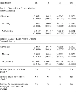
Second, we match lottery winners to marriage and divorce records filed in the years beforethe individual won the lottery. In the absence of correlation between amount won and underlying propensity to marry or divorce, we would expect no difference between the marriage and divorce rates of individuals who would later
win a large cash prize compared to those of individuals who wouldlaterwin a small cash prize. The estimated impacts of winning $25,000 to $50,000 relative to winning less than $1,000 are reported in Table A3 in the web appendix, and include estimates for the full sample as well as separate estimates for men and women. Of the 24 estimates reported, none are statistically significant at the 5 percent level, and only three are significant at the 10 percent level, which is approximately what one would expect by chance.22
20. We also estimated the model using only Fantasy 5, which has both large and small winners. Estimates of the effect of large income shocks on women’s marriage rates range from statistically significantⳮ2.6 toⳮ4.4 percentage points, compared to approximatelyⳮ3.5 percentage points reported in Table 3. 21. The significant variable was the proportion of women from the county, the coefficient of which implies that a five-percentage-point increase in the proportion of women is associated with a prize that is $325 larger. We note that this is small relative to the amounts examined in this paper.
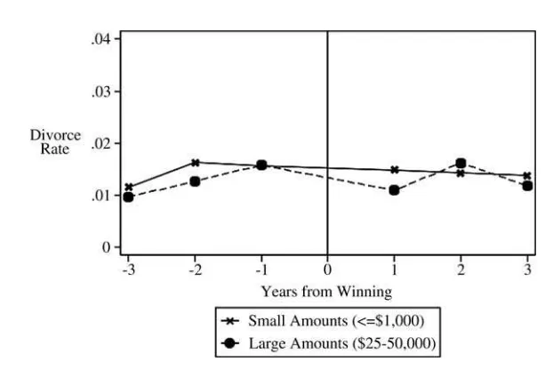
Figure 1
Flows into Divorce before and after Receiving Small and Large Cash Prizes
B. The Effect of Positive Income Shocks on Divorce
We now turn to the effect of income shocks on divorce. We begin by examining whether flows into divorce for small winners (those who won less than $1,000) are different from large winners (those who won between $25,000 and $50,000) after winning. Results are shown in Figure 1, which shows that there is little difference between the divorce rates of these two groups before or after the income shocks.
To formally test for differences in the divorce rates of the two groups in the three years after winning, we estimate Equation 1 from above. Results are shown in Table 2, in which Specification 1 indicates that the raw difference between winning $25,000 to $50,000 and winning less than $1,000 isⳮ0.39 percentage points, which is relative to a baseline divorce rate of 4.3 percent. Estimates of the effect of winning $1,000 to $10,000 and $10,000 to $25,000 are similarly small and statistically in-significant. Including controls for game, year, neighborhood, and current and pre-vious drawing payouts barely changes the estimate, as shown in Specifications 2 through 4. None of the estimates are statistically significant.
Because not all lottery players were married at the time of the income shock, the estimates must be reweighted in order to interpret the estimates as divorce rates relative to the married population. According to data from a nationally representative survey reported by Clotfelter et al. (1999) and Miami-Dade and Palm Beach county demographics, we estimate that 54 percent of lottery winners were married at the time they won. Consequently, the 4.3 percent baseline divorce rate in the lottery winner population over the three years after winning corresponds to a (4.3/0.54) 7.96 percent actual divorce rate among married individuals. Similarly, theⳮ0.39
Table 2
The Effect of Receiving Up to $50,000 on Marriage and Divorce (relative to receiving less than $1,000)
Specification (1) (2) (3) (4)
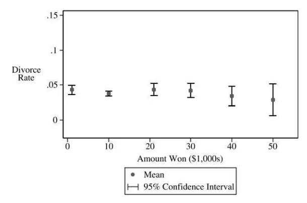
Panel 1: The Effect of Random Income Shocks on Divorce Rates within Three Years
$1,000–$10,000 ⳮ0.0032 0.0024 0.0021 0.0010 (0.0035) (0.0040) (0.0032) (0.0033)
$10,000–$25,000 ⳮ0.0025 ⳮ0.0029 ⳮ0.0027 ⳮ0.0037 (0.0048) (0.0051) (0.0043) (0.0044)
$25,000–$50,000 ⳮ0.0039 ⳮ0.0038 ⳮ0.0032 ⳮ0.0039 (0.0053) (0.0058) (0.0056) (0.0057)
Observations 40,198 40,198 40,198 38,383
Panel 2: The Effect of Random Income Shocks on Marriage Rates within Three Years
$1,000–$10,000 ⳮ0.0084 ⳮ0.0060 ⳮ0.0060 ⳮ0.0072 (0.0058) (0.0064) (0.0065) (0.0065)
$10,000–$25,000 ⳮ0.0090 ⳮ0.0093 ⳮ0.0089 ⳮ0.0099 (0.0078) (0.0083) (0.0079) (0.0085)
$25,000–$50,000 ⳮ0.0071 ⳮ0.0113 ⳮ0.0107 ⳮ0.0126 (0.0086) (0.0095) (0.0095) (0.0097)
Observations 26,629 26,629 26,629 25,539
Includes game and year fixed effects?
No Yes Yes Yes
Includes neighborhood fixed effects?
No No Yes Yes
Controls for maximum prize and total payout from previous drawing
No No No Yes
Notes: Robust standard errors are in parentheses. Estimates are relative to receiving less than $1,000 and compare to three-year divorce and marriage rates of 4.3 percent and 8.5 percent, respectively.
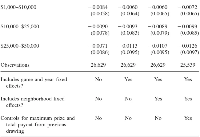
Figure 2
Observed Divorce Rates in the 3 Years after Winning the Lottery
drop in the divorce rate due to winning $25,000–$50,000. Importantly, while the estimates are not statistically different from zero, they are reasonably precise. The upper bound of the 95 percent confidence interval suggests that no more than one in 70 married couples will be induced to divorce as a result of receiving a large income shock.23This implies that to the extent life events or policy changes affect
divorce, it is unlikely due to a pure positive income shock.
To ensure that the results are not driven by the admittedly arbitrary cutoffs made in defining large and small income shocks, divorce rates for the full range of income shocks are shown in Figure 2. Consistent with the estimates in Table 2, there appears to be no relationship between the magnitude of the income shock and the likelihood of subsequently filing for divorce.
In results available upon request, we also find no difference between winners coming from minority- or majority-Hispanic zip codes, or above or below median income zip codes. We also tested whether the effect of income shocks on divorce was different by gender, which we inferred on the basis of first names using
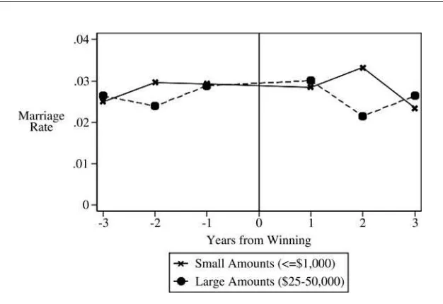
Figure 3
Flows into Marriage before and after Receiving Small and Large Cash Prizes
ical distributions of Florida schoolchildren generously provided by David Figlio.24
Results (available upon request) indicate that neither men nor women respond to income shocks on the divorce margin. The similarity of the (non)responses is con-sistent with the Coase Theorem, which predicts that changing the initial allocation of resources will only affect the settlements received by each partner, rather than the final outcome. Finally, we note that using probit to estimate the model rather than OLS yielded similar estimates.25
C. The Effect of Positive Income Shocks on Marriage
We now turn to the question of whether large positive income shocks affect an individual’s likelihood of getting married. Flows into marriage are shown in Figure 3, which indicates that consistent with the identifying assumption, there is little
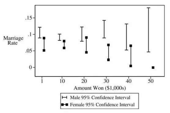
Figure 4
Observed Marriage Rates for Men and Women in the 3 Years after Winning the Lottery
difference in the marriage rates prior to the income shock. After the $25,000 to $50,000 income shock, Figure 3 also shows no definitive evidence of effects on marriage rates in the 3 years afterward. Results from more formal tests of the effect of winning $25,000 to $50,000 on marriage rates within 3 years are shown in Table 2. The marriage rates of winners of $25,000 to $50,000 are 0.7 percentage points lower than those who received less than $1,000. Adding controls increases the mag-nitude of the estimate to 1.3 percentage points. All estimates are relative to baseline marriage rates among lottery players of 8.5 percent.
To further investigate this result, we examine whether women respond differently than men.26To do so, we used empirical distributions on the gender of first names
of Florida schoolchildren provided by David Figlio to categorize 21,585 of the 26,629 individuals in the marriage data set as either male or female. The results are shown graphically in Figure 4,27while the regression estimates are shown in Table
3.28Both indicate that while positive income shocks do not affect men’s marriage
rates, women who receive $25,000 to $50,000 are significantly less likely to marry than women who receive less than $1,000. Point estimates in Specifications 1
26. We also investigate differences by income and race as proxied by the demographics of each winner’s zip code and found no differences.
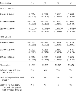
Table 3
The Effect of Receiving $25,000 to $50,000 on Three-Year Marriage Rates for Men and Women
Specification (1) (2) (3) (4)
Panel 1: Women
$1,000–$10,000 ⳮ0.0024 ⳮ0.0011 0.0010 ⳮ0.0005 (0.0100) (0.0105) (0.0104) (0.0106)
$10,000–$25,000 ⳮ0.0079 ⳮ0.0092 ⳮ0.0070 ⳮ0.0084 (0.0130) (0.0135) (0.0136) (0.0140)
$25,000–$50,000 ⳮ0.0293** ⳮ0.0341** ⳮ0.0317** ⳮ0.0342** (0.0130) (0.0137) (0.0138) (0.0140)
Panel 2: Men
$1,000–$10,000 ⳮ0.0121 ⳮ0.0112 ⳮ0.0118 ⳮ0.0126 (0.0089) (0.0095) (0.0095) (0.0096)
$10,000–$25,000 ⳮ0.0123 ⳮ0.0135 ⳮ0.0139 ⳮ0.0141 (0.0119) (0.0124) (0.0124) (0.0128)
$25,000–$50,000 0.0026 ⳮ0.0020 ⳮ0.0007 ⳮ0.0024 (0.0138) (0.0145) (0.0146) (0.0147)
Observations 21,585 21,585 21,585 20,678
Includes game and year fixed effects?
No Yes Yes Yes
Includes neighborhood fixed effects?
No No Yes Yes
Controls for maximum prize and total payout from previous drawing
No No No Yes
Notes: Robust standard errors are in parentheses. Estimates are relative to winning less than $1,000 and compare to three-year marriage rates of 7.0 percent for women and 10.6 percent for men.
through 4 of Table 3 indicate that women who receive the positive income shock are between 2.9 and 3.4 percentage points less likely to marry in the next three years than their counterparts who received less than $1,000.29 These effects are large,
representing 41 to 48 percent reductions relative to the baseline marriage rate among all female lottery players of 7 percent.
Additionally, we note that the difference between winning $25,000 to $50,000 is statistically distinguishable from the effect of winning $1,000 to $10,000 at the 1 percent level in all four specifications of Table 3. Similarly, the difference between winning $25,000 to $50,000 and winning $10,000 to $25,000 is statistically signifi-cant at the 5 percent level for Specifications 2 and 4, and at the 10 percent level for Specifications 1 and 3. This suggests it takes a relatively large income shock to induce single women not to marry.
D. Migration Out of the County of Residence
The identification strategy utilized in this paper will break down if large income shocks cause individuals to move to another county before marrying or divorc-ing.30,31We expect this to be unlikely for several reasons. First, residents of
Miami-Dade and Palm Beach counties appear to have strong roots: the Census reports that over 80 percent of residents in these counties lived in the same county five years earlier, a number which would likely be higher if not for substantial migration into the area over this time period. Second, both Miami-Dade and Palm Beach counties are very large and offer a diverse set of areas in which one could relocate without leaving the county. Geographically, Miami-Dade and Palm Beach counties cover 1,946 and 1,974 square miles, respectively, making each of them over six times the size of New York City and over one-third as large as the state of Connecticut. Both are also large in terms of population; Miami-Dade County was home to 2.3 million people in 2000 while 1.1 million people resided in Palm Beach County. Furthermore, there is substantial within-county variation in neighborhoods in both counties. For example, the median family income in the poorest zip code in Miami-Dade County was $18,000 while the median family income in the wealthiest zip code was $200,000. Collectively, these factors minimize the likelihood that a wealth shock will cause individuals to move out of the county.
29. Graphs showing flows into marriage over time for men and women separately are available in the web appendix. As shown there, the result for women appears to be driven largely by fewer marriages in the second and, to a lesser extent, third year after winning the lottery. While this pattern is not statistically precise, it is suggestive that while additional income may not cause women to cancel weddings that are already planned, it may induce women to either exit or lengthen the duration of relationships less close to marriage.
30. The potential for bias is smaller here than it might otherwise be due to how the sample was constructed. Specifically, because all individuals are assumed to not divorce (marry) unless matched to a divorce (mar-riage) record, the results are unaffected if large income shocks cause differential attrition only among individuals who will not later divorce (marry).
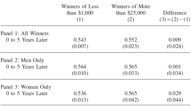
Table 4
The Proportion of Lottery Winners Who Are Linked to County Phone Records One to Five Years Later
Winners of Less than $1,000
Winners of More
than $25,000 Difference
(1) (2) (3)⳱(2)ⳮ(1)
Panel 1: All Winners
0 to 5 Years Later 0.543 0.552 0.009
(0.007) (0.023) (0.024)
Panel 2: Men Only
0 to 5 Years Later 0.564 0.565 0.001
(0.010) (0.033) (0.034)
Panel 3: Women Only
0 to 5 Years Later 0.536 0.565 0.029
(0.013) (0.042) (0.044)
Notes: Robust standard errors are in parentheses.
None of the differences are statistically different at conventional levels.
We can offer one test of whether differential migration out of the county is likely to be a problem for our analysis. Specifically, we link individuals who won the lottery between March of 2003 and March of 2007 to phone records accessed in March of 2008.32Results are reported in Table 4, which shows that the difference
in the proportion of small and big winners showing up in the county phone records zero to five years later is small and statistically insignificant. Moreover, back-of-the-envelope calculations indicate that even if we use the lower bound of the 95 percent confidence interval from attrition figures in Table 4, fully 75 percent of attriters from the county would have had to marry in other counties in order to explain the ob-served drop in marriage rates for women, a marriage rate that is 10 times that of the baseline group.33 Consequently, while this is an imperfect test due to the fact
that some households no longer have landlines, some individuals who do are not listed in the phone book, and winning the lottery could potentially enable some
32. Note that these individuals were not used in the main analysis. We are unable to use this test on the main sample of lottery winners because we do not have access to historical phone records.
families to afford a landline, it does provide comfort that differential migration from the county is unlikely to explain the results.34
VI. Discussion and Conclusions
While economists have long been interested in the relationship be-tween economic resources and marital decisions, determining the extent to which economic resources affect marriage and divorce has been difficult due to a lack of exogenous income shocks. To overcome that problem, we exploit income shocks that occur as a result of winning the lottery and compare the marriage and divorce rates of individuals who won between $25,000 and $50,000 to those who won just over $600. We find no evidence that pure income shocks cause statistically signifi-cant or economically meaningful changes in divorce rates. Moreover, even the upper bound of the 95 percent confidence interval implies that fewer than one in 70 married couples will be induced to divorce as a result of receiving an income shock that is approximately twice as large as per-capita income. However, we do find that positive income shocks reduce the likelihood that single women will marry in the following three years by 40 percent.
The combination of a large impact on women’s marriage rates and the lack of an effect on divorce rates presents an interesting puzzle. Why, after receiving a large income shock, would women avoid getting married but not exit existing marriages? Indeed, the Coase Theorem suggests that if the income shock causes total gains from being single to exceed total gains from being married, couples should not be married. This apparent contradiction can be resolved in two ways. The first relates to the role of transaction costs in marital decision-making. Although it may be optimal, after receiving the income shock, for married women to have delayed or avoided mar-riage, significant transaction costs are associated with divorce. In contrast, few, if any, transaction costs are associated with not getting married in the first place.
Alternatively, it may be that upon receiving the income shock, total welfare for a couple isnothigher unmarried than married, even though the utility of the woman may be higher if she remains single. That is, women may remain single even if that lowers the welfare of others, so long as those other parties (for example, men, children) cannot credibly promise to transfer gains from the marriage to the woman. Indeed, the social welfare implications of our finding depend crucially on why women are marrying at lower rates. On the one hand, large positive income shocks may reduce the risk-sharing benefits of marriage, or make single life more attractive in other ways. In this case, while the additional income would presumably lead to higher utility for the women, it is difficult to know how it would affect the welfare of others, such as prospective partners or children. Alternatively, it is possible that the additional wealth may enable women to postpone marriage in search of a better
match.35In that case, the income shocks may be welfare-enhancing for prospective
mates and children, as well as the single women themselves.
In examining the impact of exogenous shocks on marriage decisions, our paper fits into a much larger literature that examines the sensitivity of marriage and divorce to economic forces. Results here are broadly consistent with existing research. For example, Charles and Stephens (2004) report that while spousal job loss appears to cause divorce, spousal disability that yields a similar loss in household income does not. Charles and Stephens (2004) interpret this finding as casting doubt on a purely pecuniary motivation for divorce following a negative income shock, an interpre-tation consistent with the lack of evidence reported in this study. Similarly, while the lack of a finding on divorce in this paper contrasts with studies of welfare reform in which lower income supports are associated with lower divorce rates (Bitler et al. 2004; Hu 2003), evidence presented here suggests that the reduced divorce rates were caused by the rule changes accompanying welfare reform, rather than the change in income per se.
Our finding that random positive income shocks reduce women’s marriage rates is also broadly consistent with evidence that marriage decisions are affected by exogenous factors, including the gender of the first-born child (Dahl and Moretti 2008), minimum age requirements (Blank, Charles, and Sallee 2009), and blood test requirements (Buckles, Guldi, and Price 2009). However, our finding contrasts with the findings of other credible research designs that exploit income variation from welfare reform and report either no or weak effects on marriage (Bitler et al. 2004; Hu 2003), or exploit variation from antipoverty experiments and find higher income is correlated with higher marriage rates for single women (Gassman-Pines and Yosh-ikawa 2006). Similarly, our findings stands in contrast to Burstein’s (2007) charac-terization that studies using microdata usually find positive or no relationships be-tween women’s income and marriage (for example, McLaughlin and Lichter 1997; Smock and Manning 1997).
Our finding does not necessarily contradict these studies, however. By design, antipoverty programs and welfare reforms simultaneously changed other determi-nants of marriage, while earned income observed in other studies is likely correlated with other factors that make women attractive marriage partners. Thus, our inter-pretation is that while additional income reduces marriage rates for single women ceteris paribus, this effect may be offset by factors such as increased work require-ments that make the women more attractive mates and/or introduce them to higher-quality single men.
Collectively, our results yield two important conclusions for policy. First, it ap-pears that changing only the income of married couples will be unlikely to have an impact on the divorce margin. This indicates that to the extent policymakers wish to impact divorce rates, they ought to concern themselves primarily with the non-pecuniary determinants of marital instability. In addition, our results indicate policies that provide additional income will tend to reduce the short-term marriage rates of
single women, unless the policy is accompanied by other restrictions such as in-creased work requirements.
Table A1
Constructing the Sample of Unique Lottery Winners in Miami-Dade and Palm Beach Counties Used for Divorce Analysis
All Winners
First Time Winners
Unique in Phonebook
Amount Won Number Percent Number Percent Number Percent
⬍$l,000 7,713 10.46 5,307 9.11 3,634 9.04
$1,000–$5,000 39,151 53.11 30,794 52.89 21,383 53.19
$5,000–$10,000 16,447 22.31 13,910 23.89 9,631 23.96
$10,000–$15,000 2,130 2.89 1,810 3.11 1,191 2.96
$15,000–$25,000 3,888 5.27 3,027 5.20 2,078 5.17
$25,000–$35,000 2,938 3.99 2,263 3.89 1,524 3.79
$35,000–$50,000 1,447 1.96 1,115 1.91 757 1.88
Total 73,714 100.00 58,226 100.00 40,198 100.00
Table A2
Constructing the Sample of Unique Lottery Winners in Miami-Dade County Used for Marriage Analysis
All Winners
First Time Winners
Unique in Phonebook
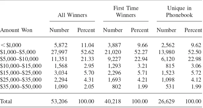
Amount Won Number Percent Number Percent Number Percent
⬍$l,000 5,872 11.04 3,887 9.66 2,562 9.62
$1,000–$5,000 27,997 52.62 21,020 52.27 13,980 52.50
$5,000–$10,000 11,351 21.33 9,227 22.94 6,120 22.98
$10,000–$15,000 1,568 2.95 1,293 3.21 815 3.06
$15,000–$25,000 3,034 5.70 2,296 5.71 1,523 5.72
$25,000–$35,000 2,294 4.31 1,693 4.21 1,098 4.12
$35,000–$50,000 1,090 2.05 802 1.99 531 1.99
Table A3
Falsification Test: The Impact of (Later) Receiving $25,000 to $50,000 on Marriage and Divorce Rates Prior to Winning
Specification (1) (2) (3) (4)
Panel 1: Divorce Rates Prior to Winning Sample/Subgroup
All winners ⳮ0.0051 ⳮ0.0053 ⳮ0.0049 ⳮ0.0050 (0.0052) (0.0057) (0.0053) (0.0055)
Men only 0.0012 0.0009 0.0016 0.0015 (0.0082) (0.0086) (0.0085) (0.0086)
Women only ⳮ0.0153* ⳮ0.0160* ⳮ0.0148* ⳮ0.0141 (0.0086) (0.0089) (0.0089) (0.0090)
Panel 2: Marriage Rates Prior to Winning Sample/Subgroup
All winners ⳮ0.0053 ⳮ0.0110 ⳮ0.0105 ⳮ0.0096 (0.0086) (0.0096) (0.0078) (0.0080)
Men only ⳮ0.0019 ⳮ0.0041 ⳮ0.0051 ⳮ0.0056 (0.0137) (0.0145) (0.0146) (0.0147)
Women only ⳮ0.0051 ⳮ0.0077 ⳮ0.0049 ⳮ0.0055 (0.0146) (0.0153) (0.0153) (0.0155)
Includes game and year fixed effects?
No Yes Yes Yes
Includes neighborhood fixed effects?
No No Yes Yes
Controls for maximum prize and total payout from previous drawing
No No No Yes
Notes: Divorce estimates for the full sample includes 40,198 observations; estimates for men and women come from a separate regression on a gender-identified sample of 33,240 observations. Marriage estimates for the full sample come from 26,629 observations; estimates for men and women come from a separate regression on a gender-identified sample of 21,585 observations. Robust standard errors are in parentheses. Estimates are relative to receiving less than $1,000 and compare to overall three-year divorce and marriage rates of 4.3 percent and 8.5 percent, respectively.
Figure A1
Flows into Marriage for Men before and after Winning the Lottery
Figure A2
References
Becker Gary S. 1981. “A Treatise on the Family.” Cambridge, Mass.: Harvard University Press.
Bitler, Marianne P., Jonah B. Gelbach, Hillary W. Hoynes, and Madeline Zavodny. 2004. “The Impact of Welfare Reform on Marriage and Divorce.”Demography41(2):213–36. Blank, Rebecca M., Kerwin Kofi Charles, and James M. Sallee. 2009. “A Cautionary Tale about the Use of Administrative Data: Evidence from Age of Marriage Laws.”American Economic Journal: Applied Economics1(2):128–49.
Buckles, Kasey S., Melanie E. Guldi, and Joseph Price. 2009. “Changing the Price of Marriage: Evidence from Blood Test Requirements.” NBER Working Paper No. 15161. Burstein, Nancy R. 2007. “Economic Influences on Marriage and Divorce.”Journal of
Policy Analysis and Management26(2):387–429.
Cain, Glen G., and Douglas A. Wissoker. 1990a. “A Reanalysis of Marital Stability in the Seattle-Denver Income-Maintenance Experiment.”American Journal of Sociology 95(5):1235–69.
Charles, Kerwin, and Melvin Stephens, Jr. 2004. “Job Displacement, Disability, and Divorce.”Journal of Labor Economics22(2):489–522.
Clotfelter, Charles, Phillip Cook, Julie Edell, and Marian Moore. 1999. “State Lotteries at the Turn of the Century: Report to the National Gambling Impact Study Commission.” Dahl, Gordon, and Enrico Moretti. 2008. “The Demand for Sons.”Review of Economic
Studies75(4):1085–120.
Edin, Kathryn. 2000. “Few Good Men: Why Poor Mothers Don’t Marry or Remarry.”The American Prospect,January: 26–31.
Gassman-Pines, A., and H. Yoshikawa. 2006. “Five-year Effects of an Anti-Poverty Program on Marriage Among Never-Married Mothers.”Journal of Policy Analysis and Management25(1):11–30.
Groeneveld, Lyle P., Nancy Brandon Tuma, and Michael T. Hannan. 1980. “The Effects of Negative Income Tax Programs on Marital Dissolution.”Journal of Human Resources 15(4):654–74.
Hankins, Scott, Mark Hoekstra, and Paige Marta Skiba. 2010. “The Ticket to Easy Street? The Financial Consequences of Winning the Lottery.”Review of Economics and Statistics.Forthcoming.
Hausman, Jerry, Jason Abrevaya, and F. M. Scott-Morton. 1998. “Misclassification of the Dependent Variable in a Discrete-Response Setting.”Journal of Econometrics, 87(2):239– 69.
Hausman, Jerry. 2001. “Mismeasured Variables in Econometric Analysis: Problems from the Right and Problems from the Left.”Journal of Economic Perspectives15(4):57–67. Hoffman, Saul D., and Greg J. Duncan. 1995. “The Effect of Incomes, Wages, and AFDC
Benefits on Marital Disruption.”Journal of Human Resources30(1):19–41. Hu, Wei-Yin. 2003. “Marriage and Economic Incentives: Evidence from a Welfare
Experiment.”Journal of Human Resources38(4):942–63.
Imbens, Guido W., Donald B. Rubin, and Bruce I. Sacerdote. 2001. “Estimating the Effect of Unearned Income on Labor Earnings, Savings, and Consumption: Evidence from a Survey of Lottery Players.”American Economic Review91(4):778–94.
Johnson, William R., and Jonathan Skinner. 1986. “Labor Supply and Marital Separation.” American Economic Review76(3):455–69.
Kearney, Melissa. 2005. “State Lotteries and Consumer Behavior.”Journal of Public Economics89(11–12):2269–99.
Laibson, David, Andrea Repetto, and Jeremy Tobacman. 2001. “A Debt Puzzle.” Working Paper.
Lindahl, Mikael. 2005. “Estimating the Effect of Income on Health and Mortality Using Lottery Prizes as an Exogenous Source of Variation in Income.”Journal of Human Resources40(1):144–68.
McLaughlin, Diane K., and Daniel T. Lichter. 1997. “Poverty and the Marital Behavior of Young Women.”Journal of Marriage and the Family59(3):582–94.
Moffitt, Robert. 1992. “Incentive Effects of the U.S. Welfare System: A Review.”Journal of Economic Literature30(1):1–61.
Schramm, David G. 2006. “Individual and Social Costs of Divorce in Utah.”Journal of Family and Economic Issues27(1):133–51.
Shapiro, Jesse M. 2005. “Is There a Daily Discount Rate? Evidence from the Food Stamp Nutrition Cycle.”Journal of Public Economics89(2–3):303–25.
Smock, Pamela J., and Wendy D. Manning. 1997. “Cohabiting Partners’ Economic Circumstances and Marriage.”Demography34(3):331–41.
Stephens, Melvin Jr. 2003 “‘3rd of the Month’: Do Social Security Recipients Smooth Consumption between Checks?”American Economic Review93(1):406–22.