BUILDING EDGE DETECTION USING SMALL-FOOTPRINT AIRBORNE
FULL-WAVEFORM LIDAR DATA
Jean-Christophe Michelin, Cl´ement Mallet, Nicolas David
IGN, MATIS, 73 avenue de Paris, 94160 Saint-Mand´e, France; Universit´e Paris-Est [email protected]
Commission III - WG III/2
KEY WORDS:Building, edge, detection, lidar, waveform, line, segmentation, diagnostic.
ABSTRACT:
The full-waveform lidar technology allows a complete access to the information related to the emitted and backscattered laser signals. Although most of the common applications of full-waveform lidar are currently dedicated to the study of forested areas, some recent studies have shown that airborne full-waveform data is relevant for urban area analysis. We extend the field to pattern recognition with a focus on retrieval. Our proposed approach combines two steps. In a first time, building edges are coarsely extracted. Then, a physical model based on the lidar equation is used to retrieve a more accurate position of the estimated edge than the size of the lidar footprint. Another consequence is the estimation of more accurate planimetric positions of the extracted echoes.
1 INTRODUCTION 1.1 Context and objectives
Information related to the emitted and backscattered laser sig-nals can be completely accessed with the full-waveform (FW) li-dar technology. Such signals gather the contribution of one or several objects that have been hit by the laser beam. An off-line post-processing step extracts maxima of the recorded sig-nals. These maxima are called ”echoes“ and will be turned into 3D points thanks to a georeferencing process. Each of them cor-responds to one or several objects closer than the sensor spa-tial resolution along the axis of the laser beam. A majority of the applications of full-waveform lidar deals with forested areas, but some recent works based on small-footprint data (diameter d < 1m) have demonstrated the relevance of lidar waveforms in urban areas, mainly for land-cover classification (Mallet et al., 2011), and vegetation detection (H¨ofle et al., 2012). The litera-ture has barely investigated the field of pattern recognition (Jutzi and Stilla, 2005b). Building edges, and more generally 3D lines, are patterns of high interest for many applications such as strip registration, building detection, change detection or database up-dating (Lee et al., 2007).
For that purpose, small-footprint lidar waveforms may be rele-vant. Typical footprint size and digitization rate are around 0.5 m and 1 GHz : each echo within the waveform is likely to cor-respond to a specific target. Information from several objects will not be mixed since the distance between the object is large enough. This is all the more interesting when detecting build-ing edges as, in case of high altimetric shift between the tar-gets, echoes will not overlap, and particular contributions may be specifically analysed.
Two issues are tackled in this paper. Firstly, we aim to detect building edges using both georeferenced 1D signals and extracted 3D points. Only linear structures are considered. Secondly, based on the assumption that building roofs are locally homogeneous in terms of geometry and radiometry, we use the knowledge of the coarse position of the edges to estimate the correct position of the 3D point within the lidar footprint, and, finally, re-estimate more precisely the 3D edge segments. In addition to the stan-dard ”waveform processing step“ which mainly add information in the altimetric component of the 3D points, our work is thus also dedicated to the planimetric improvement of the points
ex-tracted from the waveforms. This is particularly important when the lidar beam is not very focused.
1.2 Existing works
FW-based building edge detection has only be carried out in (Jutzi and Stilla, 2005a). However, plethora of papers exist when deal-ing with standard multiple-pulse lidar data. Two major kinds of approaches are possible: image and 3D-based approaches. Raster methods are mainly based on the analysis of Digital Sur-face Models (DSM) or normalized DSM (Rutzinger et al., 2009). Morphological filters, rank filters, robust hierarchical interpola-tion or gradient computainterpola-tion can be used to detect building edges. Vegetation areas are then commonly filtered by subtracting the last-echo DSM to the first-echo DSM. Classification can also be carried out by calculating the local curvature or variance of the normal vectors for each area of interest (Arefi, 2009). Further-more, theintensityoramplitudevalue may also provide discrimi-nant images for building edge detection. However, such informa-tion requires a calibrainforma-tion step (H¨ofle and Pfeifer, 2007), and has not yet been optimally used. Visible or Infra-red geospatial im-ages are therefore often preferred as complementary information (Rottensteiner et al., 2005; Matikainen et al., 2007).
The second possible approach is based on the geometrical study of the 3D point cloud. Linear features or significant vertical dis-continuities can be directly detected in the point cloud (Sampath and Shan, 2007). Such analysis can be preceded and facilitated by a building focusing step, traditionally 3D point classification as in (Zhang et al., 2006; Poullis and You, 2011). Mesh-based methods such Zhou and Neumann (2010) may allow to compute accurate edges while loosing the semantic information.
posi-tion improvement has only been tackled with real data for terres-trial datasets (Neilsen, 2011). In the proposed method, the lidar point cloud is corrected from the surface response, and particu-larly the 3D position is refined with the backscattered waveform. Unfortunately, there are major differences between aerial and ter-restrial lidar issues. This method assumes all surface to be homo-geneous within the lidar footprint, which may be inaccurate with airborne large scale data.
The paper is organised as follows. The proposed strategy will be first presented as well as the available dataset. Then, each step of the workflow will be described and commented. Finally, results will be presented, and conclusions will be drawn.
2 OVERALL STRATEGY 2.1 Methodology
The proposed methodology is based on the assumption that build-ings can be approximated by polygons,i.e., fragmented in seg-ments. Given a set of lidar measurements, our method is decom-posed into three steps:
• Step 1: Segmentation of boundary regions. Firstly, the location of building areas is coarsely retrieved, in order to decompose the problem and offer parallelization opportuni-ties. Main vegetated areas are removed and not examined in the following steps. Secondly, for each focus area, lidar waveforms are segmented in ”boundary region“ or not. The process is not limited to waveforms with multiple echoes.
• Step 2: Initial boundary extraction and diagnostic. A coarse determination of the 3D locations of the segments is first performed. 3D point clouds are first extracted from the waveforms.Then, 3D boundary segments are estimated with the standard RANSAC algorithm, adapted to deal with re-maining vegetated areas and with focus areas composed of several buildings. Finally, segments are qualified, and veg-etation points are filtered. Only the most reliable segments are fed into the adjustment process.
• Step 3 : Boundary adjustment.Based on a physical model, the positions of the 3D segments and support 3D points are improved, up to twice more accurately than the lidar foot-print.
2.2 Data
Full-waveform data has been acquired over the city of Amiens, France, in February 2008, under leaf-off conditions (OPTECH 3100-EA sensor). The point density is 2 points/m2
. We will fo-cus our study on the city center, which corresponds to 5 million backscattered waveforms covering 0.7 km2. For each lidar pulse, both emitted (pulse width = 4.8 ns) and backscattered waveforms (1 GHz digitization rate), GPS time, position and attitude of the sensor are available. Therefore, waveforms can be georeferenced, as well as 3D subsequent points (see Section 4.1).
The French national 2D topographic database is available in order to qualify the results. Thebuildinglayer has a planimetric accu-racy of around 1 m. A 0.5 m orthoimage is also used to visually assess the extraction process.
Due to the scan pattern, the 3D genuine spatial sampling of the data is not regular, which does not facilitate the local analysis, required in Section 3. Knowledge of sensor direction and posi-tion for each waveform allows to adopt asensor topologystrategy for neighbourhood computation (David et al., 2008). A georef-erenced image is created where each pixel represents the conical region of the landscape illuminated by the laser beam. One line represents one scan line, whereas one column corresponds to one angle of incidence. The major advantage of this topology is its execution time for retrieving adjacent waveforms.
2.3 Acquisition of building edges
Depending on the angle of incidence of the laser beam and the position of the sensor, edges of a building will not be all similarly acquired. Two cases can be distinguished:
• ”Single echo“ (SE): Edges corresponding to walls illumi-nated by the laser beam will create waveforms with a single echo (ground, facade or roof).
• ”Multiple echo“ (ME): The backscattered waveform is com-posed of two echoes : one on the roof, and one on the ground.
Our strategy mainly relies on the detection of ”multiple echo“ waveforms, but Step 1 is designed to retrieve all the roof wave-forms close to the gutter heights. We consider that the other lidar strips may take measures on the building from the reverse point of view, thus offering the adequate complementary information for the full contour description.
3 SEGMENTATION OF BOUNDARY REGIONS 3.1 Focus on boundary areas
The method is based of the computation of vertical discontinu-ities in 3D waveform data. For each waveform, if the vertical discontinuity is superior to a theoretical minimal building gutter height,hmin(set to 2 m to favour a high detection rate), it may lie on an edge. Computing such discontinuity as only the difference of elevation between the first and the last echoes of one waveform is not adequate, since it may discard many waveforms and pro-vide noisy results. Therefore, a 4-connexity neighborhoodV in the sensor topology is used to detect the two illumination cases.
∀w∈ W, w∈ B ⇐⇒ (Zfirstw −argmin
w∈V
Zlastw > hmin), (1)
WhereWandBare the sets of waveforms and of coarse bound-ary waveforms respectively. Zfirst(resp. Zlast) is the elevation of the first (resp. last) object hit by a given laser pulse. Such val-ues can be retrieved by detecting local maxima within the signal (e.g., Gaussian smoothing + first derivative computation). Once
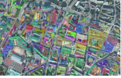
Figure 1: Results on the focusing step : one color per area.
Bis filled, a binary regular occupancy grid is generated with a resolution of 1 m. Since only a coarse segmentation is expected, this value is sufficient. The sparse grid is densified by applying a morphological closing (3×3 structuring element). Segments that may correspond to building areas are retrieved by connectivity constraint. This fast procedure allows to decompose the problem into local sub-issues.
3.2 Waveform segmentation
The goal of this part is to select waveforms from thepthfocus area (w ∈ Fp) which really lying a building edge by favouring a high detection rate. Selecting waveforms with two echoes will result in segmenting both building edges, chimneys, and vegeta-tion. The segment extraction may be highly corrupted by such false detections.
Two assumptions are made for this segmentation : the height (hi)
and the gutter line elevation (Ei) are approximately constant by
piece for theith building edge. So, for each wall, waveforms have a first echo elevation ofEi and a difference of elevation
between their first echoes and one of the echoes of their neigh-bouring waveforms ofhi. Thus, one of the major difficulties is to
computeEiandhi.
An area can contain several buildings, and in case of sloped ter-rains, may have walls with different heights. Thus, an iterative procedure should be set up, starting with the most prominent wall until finding the lowest one. In one focus area, waveforms with two echoes and largest differences of elevation between the first and the last echoes are likely to be located on building edges. Building height can then be computed among the most important differences of elevation. Since trees can be taller than buildings, the largest differences of elevation may sometimes be discarded. A rank filter is applied on the candidate waveforms: the70th per-centile (P70) is selected, and provides thehi value. Thus, for
each waveformw∈Γi(Γiis the set of waveforms which lying
theith
building edge), we have:
hi= P70
w∈Fp
({Zfirstw −Zlastw , Zfirstw 6=Zlastw}). (2)
Such value allows to select all multiple-echo waveforms that ex-hibit similar differences. A bufferχaroundhiis introduced to
gather all relevant waveforms. χis set to 0.5 m, which corre-sponds to half of the maximum variation of the wall height for a building. Moreover, the median (Md) altitude of the first echo of these waveforms is a good approximation of the elevation of the tallest gutter line (Ei).
Ei= Md w∈Fp
({Zfirstw ,|Zfirstw −Zlastw|=hi±χ}). (3)
Wall height and gutter line altitude of the tallest building in the focus area are then known. Waveforms lying on this building can now be selected. A waveformwis labelled as ”building edge“ lying onΓiif:
• Its first echo altitude is in the bufferγaround the gutter line elevationEi. γis set to 0.2 m, which is the addition of the
spatial resolution of waveforms (0.15 m), and an altimetric tolerance on the gutter line elevation (0.05 m);
• The difference of elevation between its first (or single) echo and one echo of the neighbouring waveforms (in the sensor topology, 4-connexity) is close to the wall heighthi(±χ).
∀w∈ W, w∈Γi⇐⇒
Zfirstw −argmin
w∈V
Zlastw =hi±χ
Zfirstw =Ei±γ
(4)
In practice, the procedure starts with the highest building. The corresponding waveforms are then removed, and the process iter-ates until no significant differences of elevations are found in one area.
4 INITIAL BOUNDARY EXTRACTION AND SEGMENT DIAGNOSTIC
4.1 3D point extraction
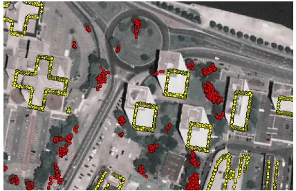
Once waveforms lying on building edges have been segmented, 3D segments can be computed. Two strategies are conceivable: processing the spatio-temporal data volume of the georeferenced waveforms as proposed in (Jutzi and Stilla, 2005b) or the 3D points extracted from the waveforms. In order to deal with large scale issues, the second possibility is selected. For that purpose, the Gaussian decomposition is performed on the waveform (Mal-let and Bretar, 2009), and only the first detected echo is preserved. Figure 2 shows the location of the extracted 3D points for an area of interest. One can notice that, building edges are well described but also that many points remain on trees. Since the following steps will deal with this problem, the segmentation step is con-sidered as satisfactory: a high true positive rate is achieved for ”building edge“ points. These ”building edge“ points are evalu-ated with the available ground truth. Around 50% of the extracted 3D points are located on building edges (Figure 2).
Figure 2: First echoes extracted from waveforms labelled as ”building edge“ in Section 3.2. Yellow (resp. red) points are located on building (resp. vegetation) areas, with respect to the ground truth.
4.2 Segment extraction
In order to fit segments on the 3D points, a robust algorithm is re-quired. These 3D points are positioned in the center of the 0.8 m lidar footprint diameter. Furthermore, for various configurations and objects (balconies, antennas etc.), multiple echoes are out-liers and may appear. The iterative RANdom SAmple Consensus (RANSAC) algorithm is appropriate to achieve this step (Fischler and Bolles, 1981). However, it has to been adapted to cope with two main issues: points located in vegetation, and separated but aligned buildings within a single focus area. For the latter case, a single segment would be extracted for two distinct buildings. Consequently, two constraints are introduced. 3D points have to fulfil both criteria to yet be considered asinliers. (cf. Figure 3, red segments).
• Orientation consistency of lines. For a given building edge, the roof is always in the same sidei.e., the vertical discon-tinuity has always the same orientation (Poullis and You, 2011). The orientation of the building edge is thus con-strained to be in the same direction along the segment. A tolerance of±45◦
is sufficient to remove false detections in vegetation. (false positive rate:59%→34%).
4.3 Boundary diagnostic
The final adjustment procedure requires a correct initialization. Furthermore, some remaining segments are still lying on vege-tated areas, and should be removed. Consequently, the boundary diagnostic is decomposed into two steps. Firstly, segments in vegetated areas are removed, and then filtered segments are di-agnosed (geometrical accuracy and reliability). The segments in vegetation areas are filtered by using two criteria:
• Planimetric scattering: Vegetated areas are known to gen-erate backscattered lidar signals with a larger width than the width of the emitted pulse (here 4.8 ns). Indeed, several ob-jects closer than the sensor range resolution will contribute to the same echo. Such echo will be wider because of the spatial extent of these targets. This is particularly true for the first echo which corresponds to the tree canopy with many material. Conversely, if the waveform hits a build-ing edge, a sbuild-ingle object will contribute to the first echo but the proportion of roof within the footprint is not suffi-cient to notice a big influence on the echo width (even if the roof is inclined). Thus, roof echoes are narrower. Con-sequently, segments where RANSAC inliers were extracted from waveform which have an average width superior to a threshold of5.5ns. Such value has been retrieved using a study of waveform widths in vegetation areas.
• Volumetric scattering: This criterion is point density-based. Vegetation generates more 3D points, that are in addition spatially scattered. A segment is labelled as ”volumetric“ whether :
N3q−Nq
Nq >0.4. (5) WhereN3qandNqare the numbers of 3D points located in a buffer respectively of 3q and q meters around the segment. This criterion is similar to (H¨ofle et al., 2012). For building areas, point density does not vary much while considering increasing areas of interest:N3q≃Nq. In this paper q=1 m so 3q is lesser than street width. The 40% increase reflects the ability of lidar beams to penetrate vegetated areas, and thus generating multiple scatterings. The buffer size has to be empirically adapted to the lidar footprint and the increas-ing rate needs to be adjusted to the point cloud density.
TRUE FALSE
TRUE 88 12
FALSE 7 93
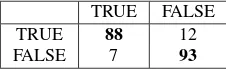
Table 1: Confusion matrix for segments corresponding to build-ing edges.
A segment is considered as ”planar“ if it fulfils these two crite-rion. Non-planar segments are removed. As illustrated wit the Table 1 and on Figure 3, the global filtering step permits to ef-ficiently remove vegetated segments. The ratio of segments in vegetation areas decreases from 34 % to 7%. Few isolated resid-ual false detections are still noticeable, but we consider that an optional regularization step that turns segments to polygonal ar-eas, posterior to our workflow, is likely to remove these errors.
The final quality of the extracted segments can be estimated with two criterion :
• Geometrical accuracy: The Root Mean Square (RMS) value is used. An segment is ”accurate“ when: RMS< 0.5d, wheredis the lidar footprint.
Figure 3: Vegetation filtering. Red segments are discarded using orientation criterion (RANSAC procedure), blue segments with planar criterion. Yellow segments are can be diagnosed.
• Reliability: A segment with a point density higher than 0.5 inlier/m is considered as ”reliable“.
The segment adjustment step is only processingaccurateand re-liablesegments.
5 BOUNDARY ADJUSTMENT 5.1 Principle
This step is inspired from the theoretical inversion on simulated data of Jutzi and Stilla (2005a). 3D extracted points have the same order of accuracy than the lidar footprint radius. The Gaus-sian decomposition permits to retrieve a correct vertical accuracy but their horizontal position need to be adjusted. For that purpose, the lidar equation (Wagner, 2010) is used and inverted to exactly find their position. A Lambertian assumption allows a clear sim-plification of this equation but is only valid for echoes lying on building roofs :
Pr= Z
t Z
τ∈ξ
K′ R4 cos (α)
ρm
CCalPe(t)d(t)d(τ), (6)
withCcal is a calibration constant,R is the range between the sensor and the target,αis the angle between the local normal of the roof and the direction of incidence of the laser beam,ξis the footprint area,PeandPrare the emitted and received power.
K′gathers other constant values. One can notes that area of the target can’t be approximated by a disk for waveforms which lying the building edge, as illustrated on Figure 5 .
Roof are locally planar and radiometrically homogeneous inside the lidar footprint, but this is not the case for ground and vegeta-tion echoes. Only first echoes are considered to adjust a segment. Our proposal method consists to iteratively :
• Use the knowledge of segment orientation to adjust its points (inliers).
• Estimate a new segment (and therefore a new orientation).
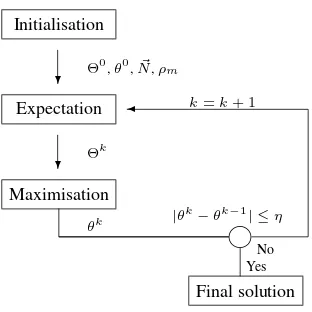
The proposed approach is a numerical Expectation-Maximisation algorithm, as illustrated in Figure 4.
5.2 Initialisation
For thejthaccurate and reliable segment (Section 4.3), the initial coarse orientation (θj0) and position (r
0
j) are already estimated in
Initialisation
❄
Expectation
❄
Maximisation Θ0
,θ0 ,N~,ρm
k=k+ 1
Θk
θk
❥
Yes
Final solution No ✛
|θk−θk−1
| ≤η
Figure 4: Iterative segment adjustment algorithm.
of pointsΘ0
jis composed of the 3D points extracted from the first
echo of waveforms lying the building edge. The local reflectance can be interpolated (up to a calibration factor) from the one echo waveforms of the neighbourhood:
∀w∈ WSE, ρm CCal =
R4
swpw
4ξ cos2
α, (7)
withswandpware, respectively, the amplitude and the width of
the echo.WSEis the set of waveforms with a single echo.
Kj′ can be estimated with one echo waveforms, lying building
roofs using:
Kj′ =
PrR
4
cos (α)ξ Pe CρmCal
. (8)
5.3 Expectation
The goal of this step is to adjust the horizontal position of points extracted from multiple-echo waveforms and located on roof edges. In a first time, the ellipsis resulting from the intersection between the laser beam and the roof plane is computed. This requires the knowledge ofN, the beam divergenceβ, the position and orien-tation of the sensor, and the standard deviation of the beamσR.
σR, in case of spatial Gaussian beam, is the distance between the
center of the line of sight and the roof, where the amplitude is divided bye2
(σR = R(2 ln 2)−1/2). The ellipsis is then
spa-tially sampled (A(τ) = 1cm2). An angular decomposition is performed in order to have a regular mesh in the orthogonal di-rection of propagation. A Kronecker testδ(τ), based on orienta-tion, is run for each cellτin order to know whether it belongs to the roof.
Roof R
~ N α
hj
δ(τ) = 1
δ(τ) = 0
Figure 5: Illustration of the iterative segment adjustment algo-rithm.
In a second time, the laser beam is temporally sampled (1 GHz). For a fixed timet, the intersection between each discretized ray
and the roof is computed. Then, the associated transmitted inci-dent power for each cell can be calculated:
Pt(t, τ) =Pe(t)c(R)A(τ) exp
−d2
2σ2
R
δ(τ),
wheredis the orthogonal distance between the laser beam axis and the intersection between the discretized ray and the roof, c(R)is the amplitude diminution factor due to the distanceR between the sensor and the roof. For each discretized ray integra-tion, the associated backscattered powerPrth can be calculated
by using the simplified lidar equation (Mallet and Bretar, 2009):
Prth=
R tK
′′
cos (α)R2ρm
CCalPt(t)d(t),
whereK′′is a constant which depends on the wavelength and the aperture of the laser. By an integration over time, the backscat-tered power of each laser beam is known.
With the fixed orientation,θk−1
j , different positions of the
build-ing edge are simulated for the given ellipsis position. Calcu-lated backscattered powersPrth are compared to the measured
backscattered power Pr. The position of the good simulated
building edge is obtained when the sign of (Prth−Pr) change. The adjusted point is positioned in the orthogonal position to the laser beam axis on the good simulated position of the building edge.
5.4 Maximisation
Adjusted segment can be computed on the set of adjusted points with a least-square algorithm (Θj). Then, the new orientationθjk
and position arerkj derived. Such value can be used to iterate on
the 3D point positions. The algorithm stops when the change of the orientation is negligible (η= 5o).
As illustrated on Figure 6, the adjusted segment has a better ac-curacy (in average the RMS decrease by 0.15 m).
Figure 6: Adjustment results. Extracted points before adjustment (red), after adjustment (green). Segment RMS decreases from 0.37 to 0.27 m.
6 RESULTS
vertical distance between each side of these edges is not impor-tant enough.
Segment adjustment results are less exhaustive (about 5%). The major parts of segments cannot be adjusted because the one ma-terial planar roof is a too restrictive assumption. However, when the procedure is possible, the extraction is improved: the RMS increases of 0.15 m, which is satisfactory with respect to the foot-print radius (0.4 m).
Figure 7 provides an overview of the full process applied to the whole dataset. One can notice that once results from different strips are merged, building are correctly outlined.
Figure 7: Extracted feature before vegetation filtering : one colour per strip.
7 CONCLUSION
Building edge detection using airborne full-waveform lidar is a problem which have never been addressed with real data before. The approach described in this paper proposes a solution provid-ing reliable boundaries segments with very low false positive rate. We have tried to benefit from the particular specification of the acquisition process with 0.8 m footprint size, delivering a large number of waveforms with multiple and well separated echoes. The algorithm is decomposed into several independent parts that can be easily tuned to fit to the specification of other surveys. The main concern of the paper was to provide fast methods to be able to efficiently process large amount of data.
The first limitation of the proposed approach is that only seg-ments are considered. However, other primitives (such as circles, curves) may be inserted for specific landscapes. One just has to add a model selection step within the RANSAC procedure. Fur-thermore, the adjustment step is limited because of the too strict roof modelling. Future work focusing therefore in improving the roof reflection model, by providing a more complete mathemat-ical formulation. This would increase the rate of adjusted prim-itives, and being quantitatively assessed with simulated datasets. Finally, it would be interest to add a final step that would turn the set of adjusted primitives into polygons to obtain geometric forms similar to cadastral data.
References
Arefi, H., 2009. From lidar point clouds to 3D building models. PhD thesis, Universit¨at der Bundeswehr M¨unchen, Institut f¨ur Angewandte Informatik, Germany.
David, N., Mallet, C. and Bretar, F., 2008. Library concept and design for lidar data processing. International Archives of the Photogrammetry, Remote Sensing and Spatial Information Sciences, 38 (Part 4-C1), (on CD-ROM).
Fischler, M. and Bolles, R., 1981. Random sample consensus: A paradigm for model fitting with applications to image analy-sis and automated cartography. Communications of the ACM 24(6), pp. 381–395.
H¨ofle, B. and Pfeifer, N., 2007. Correction of laser scanning in-tensity data: Data and model-driven approaches. ISPRS Jour-nal of Photogrammetry and Remote Sensing 62(6), pp. 415– 433.
H¨ofle, B., Hollaus, M. and Hagenauer, J., 2012. Urban vegetation detection using radiometrically calibrated small-footprint full-waveform airborne lidar data. ISPRS Journal of Photogram-metry and Remote Sensing 67, pp. 134–147.
Jutzi, B. and Stilla, U., 2005a. Sub-pixel edge localization based on laser waveform analysis. The International Archives of the Photogrammetry, Remote Sensing and Spatial Information Sciences 36 (Part XX), pp. 109–114.
Jutzi, B. and Stilla, U., 2005b. Waveform processing of laser pulses for reconstruction of surfaces in urban areas. The Inter-national Archives of the Photogrammetry, Remote Sensing and Spatial Information Sciences 31 (Part 8/W27), (on CD-ROM).
Lee, J., Yu, Y., Kim, Y. and Habib, A., 2007. Adjustment of discrepancies between lidar data strips using linear features. IEEE Geoscience and Remote Sensing Letters 4(3), pp. 475– 479.
Mallet, C. and Bretar, F., 2009. Full-waveform topographic lidar : State-of-art. ISPRS Journal of Photogrammetry and Remote Sensing 64(1), pp. 1–16.
Mallet, C., Bretar, F., Roux, M., Soergel, U. and Heipke, C., 2011. Relevance assessment of full-waveform lidar data for urban area classification. ISPRS Journal of Photogrammetry and Remote Sensing 66(6), pp. S71–S84.
Matikainen, L., Kaartinen, H. and Hyypp¨a, J., 2007. Classifica-tion tree-based buidling detecClassifica-tion from laser scanner and aerial image data. The International Archives of the Photogramme-try, Remote Sensing and Spatial Information Sciences, 36 (Part 3/W52), (on CD-ROM).
Neilsen, K., 2011. Signal processing on digitalized ladar wave-forms for enhanced resolution on surface edges. Master’s the-sis, Utah State University, USA.
Poullis, C. and You, S., 2011. 3d reconstruction of urban areas. In: Proc. of IEEE 3DIMPVT, Hangzhou, China.
Rottensteiner, F., Summer, G., Trinder, J., Clode, S. and Ku-bik, K., 2005. Evaluation of a method for fusing lidar data and mulitspectral images for building detection. International Archives of the Photogrammetry, Remote Sensing and Spatial Information Sciences 36 (Part 3/W24), pp. 15–20.
Rutzinger, M., Rottensteiner, F. and Pfeifer, N., 2009. A com-parison of evaluation techniques for building extraction from airborne laser scanning. IEEE Journal of Selected Topics in Applied Earth Observations and Remote Sensing 2(1), pp. 11– 20.
Sampath, A. and Shan, J., 2007. Building boundary tracing and regularization from airborne lidar point clouds. PE&RS 73(7), pp. 805–812.
Wagner, W., 2010. Radiometric calibration of small footprint full-waveform airbone laser scanner measurements: Basic physical concepts. ISPRS Journal of Photogrammetry and Re-mote Sensing 65(6), pp. 505–513.
Zhang, K., Yan, J. and Chen, S.-C., 2006. Automatic construction of building footprints from airborne lidar data. IEEE TGRS 44(6), pp. 2523–2533.