Proceedings of Slope 2015, September 27-30th 2015
THE INFLUENCE OF DYNAMIC ACCELERATION OF SINUSOIDAL LOADS TO
THE LANDSLIDE SURFACE OF CANTILEVER RETAINING WALLS
Anissa M.Hidayati 1, Sri Prabandiyani RW 2 and I Wayan Redana 3
ABSTRACT: The dynamic acceleration is one of dynamic parameters will be taken into consideration in the analysis of the safety of retaining wall construction due to dynamic loads beside other parameters such as: (1) the dynamic frequency, (2) the density of soils and (3) the amplitude of vibration. This research aims to study the role of dynamic acceleration to the landslide surface of retaining walls of cantilecer type due to dynamic load. This study was done by a small scale model test of cantilever retaining wall type of 18 centimeters in height, 9 centimeters in width and loaded by using shaking table to simulate dynamic loads. The dynamic load was given with the variation of the frequency and amplitude of vibration to obtain the acceleration of dynamic response. The dynamic acceleration response was measured by using accelerometer. Dry sand with three densities variations were used in this experiment. The movements of the sand grains were recorded during experiment to be able to show the change of the sliding surface of the retaining wall. The results showed that there was the difference in the dynamic acceleration response generated due to differences in the dynamic frequency and amplitude of vibration.There was also a relation ship between the value of dynamic acceleration response to the shape of the landslide surface.
Keywords: dynamic acceleration response, landslide surface, soils density, cantilever type
1 Student, Udayana University, [email protected], INDONESIA 2 Professor, Diponegoro University, [email protected], INDONESIA 3 Professor, Udayana University, [email protected], INDONESIA
INTRODUCTION
Landslides occur on a regular basis throughout the world as part of the ongoing evolution of landscapes. Many landslides occur in natural slopes, but slides also occur in man-made slopes from time to time. At any point in time, then, slopes exist in states ranging from very stable to marginally stable. When earthquake occur, the effects of earthquake-induced ground shaking is often sufficient to cause failure of slopes that were marginally to moderately stable before the earthquake. The resulting damage can range from insignificant to catastrophic depending on the geometric and material characteristics of the slope. Construction of retaining wall construction is one way to anticipate the slopes damage due to earthquake load.
In the last two decades had developed innovative system which was used to anticipate the damage of slopes caused by the earthquake. In general, ground anchoring system for seismic design purposes can be divided into three main categories: gravity walls, cantilever walls and braced walls. Each type of wall
posses different assumption in evaluating lateral soil pressure.
Retaining walls can fail in many difference ways. Cantilever walls fail by sliding, overturning, or gross instability also fail in bending. The magnitude and distribution of dynamic wall pressures were influenced by the mode of wall movement, e.g., translation , rotation about the base, or rotation about the top (Sherif, A. M., and Fang, Y - S. 1984).
walls (Sherif and Fang 1984). The experimental results showed that the distribution of dynamic active earth pressure as a function of acceleration. Dynamic active ground pressure distribution obtained from the value of soil pressure of observe by using transducer, hence pressure did not calculating by using the real movement of soil particle of the experiment. Dynamic active pressure increased with the increased in acceleration. Ishibashi and Fang (1987) completed the rigid retaining wall stability issues using a combination of analytical methods based on displacement and experimental methods. The experiments carried out used a shaking table with model of gravity wall. The experiments were done on dry soils and non-cohesive, while the walls were allowed to experience a variety of movements such as translation, rotation of the bottom wall, the rotation at the top of the wall, and combinations thereof. When the rotation at the base of the wall, the pressure distribution is not linear. In the area near the base of the wall, there is a high residual stress due to displacement of the wall, hence the capture point of active pressure is lower than a third of the wall height. When the rotation at the top of the wall, the pressure distribution is not linear. There are areas that had a high stress near the top of the wall as a result of the tapered land, and the area had a low voltage at the base of the wall due to a shift in the wall. Consequently, capture point total active dynamic pressure was higher than a third of the wall height. Dynamic lateral earth pressure distribution obtained from observations on the value of soil pressure transducer.
LITERATURE REVIEW
Construction of the building both inside or on the surface of the ground, not only accepted static load but also dynamic load. Dynamic load acting on the land or building structures could be derived from natural or man-made. If the dynamic loads worked on the ground, it would caused the movement of soil grain, consequently the structure which was supported by the soil would experienced instability.
Dynamic Response of retaining wall ranging from even the simplest to quite complex. Movement and pressure of the wall depends on the response of the soil which underlying of walls, the response of the back-fill, the response of inertia and flexibility of the wall itself, and the nature of the input motion (Kramer, Steven L. 1996).
The problem of retaining soil is one of the oldest in geotechnical engineering; some of the earliest and most fundamental principles of soil mechanics were developed to allow rational design of retaining walls.
Many different approaches to soil retention have been developed and used successfully.
Seismic design of retaining walls is generally based on seismic pressure or allowable displacement. In the former approach, static or pseudo-dynamic analysis are used to estimate seismically induced wall pressure, and the wall is designed to resist those pressure without failing or causing failure of the surrounding soil. The latter approach involves designing the wall such that its seismically induced permanent displacement does not exceed a predetermined allowable displacement.
Modeling experiments in the laboratory can be done with the aim to study the movement of sand and retaining wall caused by vibration (dynamic load) using cantilevered retaining wall models that are supported by dry sand with provided dynamic load (sinusoidal) with variations of the vibration acceleration and the density of the sand.
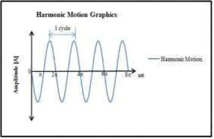
The objects that perform accelerated uniformly motion, has fixed acceleration, this means that the object is always working with pattern that remains both direction and magnitude. If it’s force is always changing, the acceleration is olso changing. Repetitive motion in the same time interval called a periodic motion. This periodic motion occurs on a regular basis and motive force is proportional to the amplitude. Easy to understand that the smaller the amplitude is also smaller the driving force. The largest amplitude is called amplitude of vibration (A). Periodic motion can be expressed in sine or cosine function, therefore periodic motion is called harmonic motion. The periodic motion that moves back and forth through the same trajectory so-called vibration or oscillation and is also known as a simple harmonic motion. The time needed to take the path back and forth is called the period, while the number of vibrations per unit time is called frequency. The relationship between the period (T) and frequency (f) according to this statement is expressed as the equation 1.
1 [sec] f
T (1)
The frequency (f) or the amount of vibration in each unit time is expressed in equation 2.
1 [cps] T
f (2)
While the mathematical function from objects called harmonic motion/vibration (Prakash, S., 1981)
xAsin(t) (3)
where x is the displacement of a trajectory in function
of time (t); A is the amplitude (equal to the maximum
displacement); ω is the angular frequency of the trajectory [radians/sec]; t is the time [seconds]. The
harmonic motion repeated every 2π radians with fixed angular velocity and maximum displacement is value of A, referred to as amplitude (Figure 1.).
Figure 1. Representation fo harmonic motion.
A cycle of motion is completed when the movement reached one full rotation as described in equation 4.
2 f [radians/sec] (4)
with f is frequency of vibration.
From equation 4., values of obtained f as defined in equation 5.
cps f
2
(5)
To determine the velocity of simple harmonic motion, differentiate equation 3. with respect to time (t) in order to obtain equation 6 (Prakash, S., and Puri, V. K., 1988).
(Asin t) Acos( t) dt
d
dt dx
x (6)
where
x
is the velocity of simple harmonic motion equation. Then, to obtain the acceleration of simple harmonic motion by differentiating equation 6. with respect to time (t) thus produce equation 7.a x t A t A dt
d
dt x d
x ( cos( )) 2sin( )2
(7)
where
x
is the acceleration of simple harmonic motion equation, also denoted as a. The displacement path, velocity and acceleration of motion was described in Figure 2.By taking into account the movement of grain movement graphic results, it can be calculated the area of landslide behind the retaining wall construction due to the sinusoidal dynamic load (see Figure 3.).
Figure 2. Representation of displacement, velocity and acceleration
Figure 3. The area bounded by curve y1 = f(x), y2 =
f(x), x = 0 dan x = x1
The area bounded by 2 (two) curves y1 and y2 which
as function of x and x = 0 and x = x1, it can be
calculated:
The area below of curve y1, x = 0 and x = x1 is
expressed as equation 8.
A
y
dx
x
10 1
1 (8)
The area below of curve y2, x = 0 and x = x1 is
defined in equation 9.
A
y
dx
x
20 2
1 (9)
A
A
A
y
dx
y
dx
See the segment of y x dx. Then the centroid segment against X-axis and Y-axis is C (
x;
y
). The of coordinates centroid C can be obtained by using equation 11 and equation 12.The Laboratory Soil Mechanics of Civil Engineering Faculty, Udayana University, Bali, Indonesia. The model of retaining wall was made of concrete placed on dry sand. Model test was performed using dry sand material with a grain size through No. 4 of sieve and retained No.100 sieve of loose sand density (DR = 30 %), medium sand density (DR = 55 %) and dense sand density (DR = 70 %). The model of retaining wall was designed as a cantilever type of 18 centimeters in height (H), 9 centimeters in width (B). The model retaining wall was loaded by sinusoidal speed and amplitude variations. Dynamic response was recorded using recording devices vibration acceleration (accelerometer). During experiment the movement of sand grains recorded.
The model tests was made in the glass box of 2 meters in length, 0.4 meter in width and 1 meter in height. Thick of glass box was 10 millimeters. The glass box was placed on a vibrating table (shaking table) supported by four wheels. Shaking table was driven by an electric motor through two pulleys that drive the crank shaft that was connected to the connecting rod that was prepared as shown in Figure 4. Shaking table moved back and forward horizontally with a given variant of speed (inverter).
Figure 4 The equipment of retaining walls model test on sinusoidal dynamic load (not scaled) (Hidayati et
al. 2015)
DATA COLLECTION AND DISCUSSION
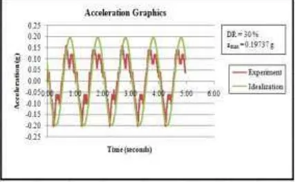
A model experiment was carried out as many as 6 units with details of 2 experiments with low density DR 30%, 3 experiments were the medium density DR = 55% and an experiment with high density Dr = 70%. The shaking table vibrated with speed variation. In the experiment of 30% in density (DR = 30 %) with variations of the amplitude and frequency obtained dynamic acceleration response graphics as shown in Figure 5, Figure 6 and Figure 7.
The Results of recorded of the shaking table movement was obtained in the form of the dynamic acceleration response graphics. The graph further idealized by using equation 1. through equation 7., also to obtain the value of the maximum dynamic acceleration response that occured. The first experiments carried out of 0.005 meter in the amplitude of vibration and one cicle per second in the frequency of vibration.
Figure 5. Dynamic acceleration response graph of cantilever model of A= 0,005m, DR = 30 %
conducted by using the same density that DR = 30% and the results are shown in Figure 6.
Figure 6. Dynamic acceleration response graph of cantilever model of A= 0,0081m, DR = 30 %
Figure 6. shows that of 0.0081 meter in amplitude and 0.83 cicle per second in frequency obtained of 0.22029 g in the maximum dynamic acceleration. It shows that the increase in the amplitude of vibration with decrease in the frequency of vibration can lead to a decrease in the maximum dynamic acceleration vibration. Then next experiments carried out additional of 15 percents in frequency with 0.005 meter in amplitude and the results are presented in Figure 7.
Figure 7. Acceleration response graph of cantilever model of A= 0,005m, DR = 30 %
Figure 7. shows that if the results of the experiment in figure 5. compared to experimental results of 0.005 meter in amplitude and 1.15 cicles per second in frequency as in figure 7. with 0.26105 g in maximum dynamic acceleration indicates that the increase of 15 percent in frequency with the same amplitude resulted an increase of maximum dynamic acceleration about 32.32 percent. This indicates that the maximum dynamic acceleration is only influenced by the frequency of vibration. The role of the vibration frequency and amplitude of vibration to the dynamic acceleration response presented in Figure 8
Figure 8. The graph of the dynamic acceleration response with amplitude, frequency variations to
density of DR = 30 %
Figure 8. shows that by increasing the amplitude of vibration by 62 percent accompanied by lowering the vibration frequency of about 17 percent then the maximum dynamic acceleration increased 11.61 percent. Dynamic acceleration increased 18.5 percent if the vibration amplitude decreased 38.3 percent but the vibration frequency increased 38.5 percent. If the vibration frequency is increased to 15 percent by the amplitude remains the maximum dynamic acceleration increased 32.26 percent.
Experiment with medium density DR = 55%, with the amplitude and frequency variations obtained the dynamic acceleration response graph as shown in Figure 9, figure 10 and Figure 11.
Figure 9. Acceleration response graph of cantilever model of A= 0,005m, DR = 55 %
Figure 10. Acceleration response graph of cantilever model of A= 0,0055 m, DR = 55 %
Figure 10 shows that the maximum dynamic acceleration reached 0.35742 g with increased the amplitude of vibration becomes 0.0055 meter and the vibration frequency to 1.3 cicles per second.
In the next experiment with increasing the amplitude becomes 0.0104 meters but the frequency was reduced to 0.95 cicle per second obtained the maximum dynamic acceleration by 0.37767 g as shown in Figure 11.
Figure 11. Acceleration response graph of cantilever model of A= 0,0106 m, DR = 55 %
The influence of vibration amplitude and frequency of vibration to the maximum dynamic acceleration with a density of DR = 55% can be seen in Figure 12.
Figure 12. The graph of the dynamic acceleration response with amplitude, frequency variations to
density of DR = 55 %
Figure 12. shows that by increasing the amplitude of vibration by 10 percent accompanied by increasing the vibration frequency about 13 percent then the maximum dynamic acceleration increased 36.54 percent. Dynamic acceleration increased about 6 percent if the vibration amplitude increased but the vibration frequency decreased respectively about 27 percent. If the vibration frequency is increased to 112 percent but the amplitude decreased to about 17 percent then the maximum dynamic acceleration increased about 45 percent.
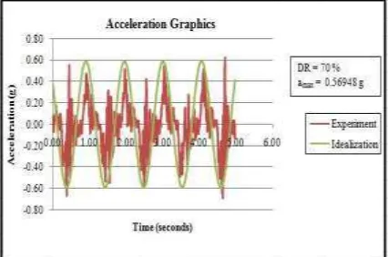
The last experiment with high density DR = 70 % had done of 0.0165 in the vibration amplitude and 0.95 cicle per second in the vibration frequency as shown in Figure 13.
Figure 13. Acceleration response graph of cantilever model of A= 0,0165 m, DR = 70 %
Figure 13. shows that with gave of 0.0165 meter in amplitude of vibration and 0.95 cicle per second in frequency of vibration to DR = 70 % in high density obtained 0.56948 g in maximum dynamic acceleration. The maximum dynamic acceleration values obtained from all of experiments with density, amplitude and frequency variations is shown in tables 1.
Table 1. Dynamic acceleration response of the tests
No of test
DR [%]
A [m] f [cps] amax [g]
1 30 0.005 1 0.19737 2 30 0.0081 0.83 0.22029 3 30 0.005 1.15 0.26105 4 55 0.005 1.15 0.26104 5 55 0.0055 1.3 0.35642 6 55 0.0106 0.95 0.37767 7 70 0.0165 0.95 0.56948
landslides areas used equations 11. The shape of landslide and the centroid coordinates of landslide to experiment of DR = 30 % in density is presented in the Figure 14, DR = 55 % in density in the Figure 15 and DR = 70 % in density in Figure 16.
Figure 14. The graph of shape and centroid of slide surface, DR = 30 %
Figure 14. shows that increasing the maximum the dynamic acceleration of 18.5% gives a result of the greater bandwidth landslide five-times. Centroid coordinates trends tend toward the horizontal. Furthermore, the shape of coordinates of landslides areas and the centroid of landslide areas to experiment with DR = 55% in density is presented in Figure 15.
Figure 15. The graph of shape and centroid of slide surface, DR = 55 %
Figure 15 shows that increasing the maximum the dynamic acceleration provides greater the bandwidth due to landslide but smaller than the density of DR = 30%. Centroid coordinates trends tend vertical direction. Next, the form of landslides areas and coordinates of landslides areas to experiment with a density DR = 70% is presented in Figure 16.
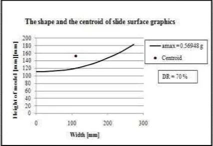
Figure 16. The graph of shape and centroid of slide surface, DR = 70 %
Figure 16 shows that by provides maximum dynamic acceleration of 0.56948 g, the bandwidth of landslide that occurs very small compared to other experiments with the maximum dynamic acceleration which is smaller.
The equation of landslides, the areas of landslides, the height of landslides areas, the width of landslides areas and the centroid of landslides areas are presented in Table 2.
Table 2. Area of landslides of the tests
No of test
DR [%]
Slide function Area [cm2]
Height [h] of
slide (x H)
Width [b] of slide (x H)
Centroid of slide [mm];
(xc, yc)
1 30 y = 181.9569 0 - - -
2 30 y =6E-07x3+0.001x2–0.057x +141.5 32.50 0.1407 0.9674 68.71; 155.38
3 30 y =0.168x +97.95 202.19 0.4091 2.3118 156.24; 153.08 4 55 y =0.002x2-0.135x +106.4 109.04 0.3878 1.2477 85.16; 144.29
5 55 y = 0.002x2-0.115x +48.31 249.45 0.7317 1.5069 106.52; 121.03
6 55 y =6E-10x4-3E-07x3+0.196x+0.156 564.01 1.0056 2.3656 187.3; 105.4
CONCLUSION
Based on the data which obtained during this experiment, the following conclusions can be drawn about the influence of dynamic acceleration of sinusoidal loads to the landslide surface of cantilever retaining walls:
1. Dynamic Acceleration is a function of vibration frequency and amplitude of vibration. So the value of dynamic acceleration is directly proportional to the frequency of vibration and amplitude of vibration
2. Increasing the percentage of vibration frequency with fixed vibration amplitude resulting in increasing of the percentage of the maximum dynamic acceleration in double of the vibration frequency percentage
3. Addition of the percentage of the amplitude of vibration with remained in vibration frequency resulting in increasing of the maximum dynamic acceleration which equal to the percentage of increasing the amplitude of vibration
4. The size of landslides area that occurred during experiment showing direct proportion to the maximum dynamic acceleration which is given at a certain density
5. The form of landslides area that occurred showing direct proportion to the dynamic acceleration which is given at a certain density
6. Centroid coordinates followed the pattern of landslides area
7. By increasing of 18.5% in the maximum the dynamic acceleration with density of sands DR = 30 %.gives a result of the greater area of landslide five-times and centroid coordinates trends tend to more flat
8. By increasing to DR = 55 % and by increasing the maximum of the dynamic acceleration provides greater of the size of landslide, however the size of landslide is smaller compere to the density of DR = 30 % as expected. The centroid coordinates trends tend incline toward vertical.
REFERENCES
Hidayati, A. M., Prabandiyani, S. RW., and Redana, I.W. Laboratory Tests on Failure of Retaining Walls Caused by Sinusoidal Load. Applied Mechanics and Materials Vol 776 (2015) pp 41-46, © (2015) Trans Tech Publications, Switzerland, doi:10.4028/www.scientific.net /AMM.776.41.
Ishibashi, I. and Fang, Y – S ., 1987. Dynamic Earth Pressures with Different Wall Movement Modes. Soils And Foundations, Vol. 27, N0. 4, 11-22, Dec. 1987, Japanese Society Of Soil Mechanics And Foundation Engineering.
Kramer, Steven L. 1996. Geotechnicl Earthquake Engineering. Upper Saddle River, New Jersey 07458: Prentice Hall, Inc.
Mononobe, N., and Matsuo, H., 1929. On Determination of Earth Pressure during Earthquake. Proccedings World Engineering Conference, Tokyo, Japan, Vol. 9.
Okabe, S., 1924. General Theory of Earth Pressure and seismic Stability of Retaining Wall and Dam. Journal of Japanese Soc. of Civil Engineering, Vol. 10, No. 6.
Prakash, S., 1981. Soil Dynamics. McGraw-Hill, Inc. Prakash, S., and Puri, V. K., 1988. Foundations for
Machines : Analysis and Design. John Wiley & Sons, Inc.