CHAPTER 4
Analysis of cross-classifications using Crosstabs
The crosstabulation table is the basic technique for examining the relationship between two categorical (nominalor ordinal) variables, possibly controlling for additional layering variables.
The Crosstabs procedure offers tests of independence and measures of association and agreement for nominal and ordinal data. You can also obtain estimates of the relative risk of an event given the presence or absence of a particular characteristic, and you can test for significant differences in column proportions in the crosstabulation table.
4.1. Using Crosstabs to study nominal-by-nominal relationships
In order to determine customer satisfaction rates, a retail company conducted surveys of 582 customers at 4 store locations. From the survey results, you found that the quality of customer service was the most important factor to a customer's overall satisfaction. Given this information, you want to test whether each of the store locations provides a similar and adequate level of customer service.
The results of the survey are stored in satisf.sav. See the topic Sample Files for more information. Use the Crosstabs procedure to test the hypothesis that the levels of service satisfaction are constant across stores.
4.1.1. Running the analysis
Figure 36 Crosstabs dialog box
2. Select Store as the row variable.
3. Select Service satisfaction as the column variable. 4. Click Statistics.
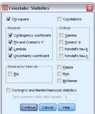
Figure 37 Statistics dialog box
5. Select Chi-square, Contingency Coefficient, Phi and Cramer's V, Lambda, and Uncertainty coefficient.
6. Click Continue.
4.1.2. Crosstabulation table
Figure 38 Crosstabulation for Store by Service satisfaction
The crosstabulation shows the frequency of each response at each store location. If each store location provides a similar level of service, the pattern of responses should be similar across stores.
At each store, the majority of responses occur in the middle. Store 2 appears to have fewer satisfied customers.
Store 3 appears to have fewer dissatisfied customers.
From the crosstabulation alone, it's impossible to tell whether these differences are real or due to chance variation. Check the chi-square test to be sure.
4.1.3. Chi-square tests
Figure 39 Chi-square tests for Store by Service satisfaction
The chi-square test measures the discrepancy between the observed cell counts and what you would expect if the rows and columns were unrelated. The two-sided asymptotic significance of the chi-square statistic is greater than 0.10, so it's safe to say that the differences are due to chance variation, which implies that each store offers the same level of customer service.
actual quality of service at a store, so you further cross-classify by whether they had contact with a service representative.
4.1.4. Adding contact with employee as a layer variable
1. Recall the Crosstabs dialog box.
2. Select Contact with employee as a layer variable. 3. Click OK in the Crosstabs dialog box.
4.1.4.1. Crosstabulation table
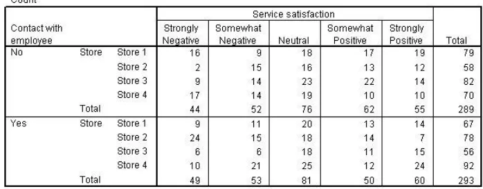
Figure 40 Crosstabulation for Store by Service satisfaction, controlling for Contact
The crosstabulation now splits the previous crosstabulation into two parts. Now that the customers who didn't have contact are sorted out, there appears to be a significant association between store 2 and low service satisfaction. Check the chi-square test to be sure.
4.1.4.2. Chi-square tests
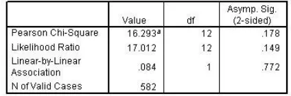
Figure 41 Chi-square tests for Store by Service satisfaction, controlling for Contact
The significance value of the test for customers who did not have contact is 0.052. This is suggestive, but not conclusive, evidence of a relationship between Store and Service satisfaction for these customers. While not directly related to the quality of service given by your employees, you might consider a separate analysis of these customers to determine if there is some other factor that accounts for this relationship.
The significance value of the test for customers who had contact with an employee is 0.012. Since this value is less than 0.05, you can conclude that the relationship observed in the crosstabulation is real and not due to chance.
While the chi-square test is useful for determining whether there is a relationship, it doesn't tell you the strength of the relationship. Symmetric measures attempt to quantify this.
4.1.4.3. Symmetric measures
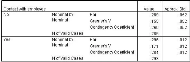
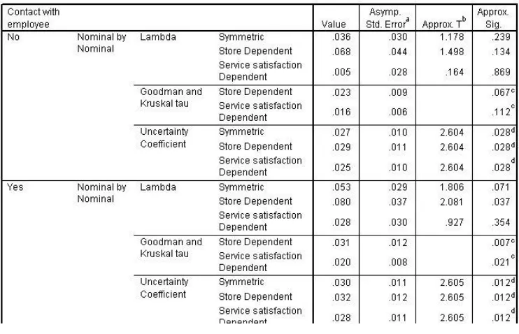
Figure 42 Symmetric measures for Store by Service satisfaction, controlling for Contact
Symmetric measures are reported separately for customers who did and did not have contact with a store representative. These measures are based on the chi-square statistic.
Phi is the ratio of the chi-square statistic to the weighted total
Cramer's V is a rescaling of phi so that its maximum possible value
is always 1. As the number of rows and columns increases, Cramer's V becomes more conservative with respect to phi.
The contingency coefficient takes values between 0 and SQRT[(k-1)/k], where k = the number of rows or columns, whichever is smaller. It becomes more conservative with respect to phi as the associations between the variables become stronger. The significance values of all three measures are 0.012, indicating a statistically significant relationship. However, the values of all three measures are under 0.3, so although the relationship is not due to chance, it is also not very strong.
While these measures give some sense of the strength of the association, they do not, in general, have an intuitive interpretation. To develop a clearer sense of this, look at the directional measures.
4.1.4.4. Directional measures
Directional measures quantify the reduction in the error of predicting the row variable value when you know the column variable value, or vice versa. Each measure simply has a different definition of "error."
Lambda defines error as the misclassification of cases, and cases
are classified according to the modal (most frequent) category. Tau defines error as the misclassification of a case, and cases are
classified into category j with probability equal to the observed frequency of category j.
The uncertainty coefficient defines error as the entropy, or P(category j) * ln(P(category j)) summed over the categories of the variable. The uncertainty coefficient is also known as Theil's U. For customers who had contact, the Goodman and Kruskal's tau value of 0.031 with Store dependent means that there is a 3.1% reduction in misclassification. The other measures report equally small values, indicating that the association between Store and Service satisfaction is almost solely due to the poor service at store 2.
4.1.5. Summary
Using Crosstabs' nominal-by-nominal measures, you initially found that each store offers a similar quality of customer service. However, once customers who did not have contact with a service representative were separated out, a relationship between Store and Service satisfaction emerged. Fortunately, that relationship is rather weak, indicating that while there is a measurable difference in the service quality between stores, it is likely due to the poor service of a single store rather than a more serious company-wide variation in store image.
4.2. Using Crosstabs to study ordinal-by-ordinal relationships
A retail company that conducted a customer satisfaction survey is interested in learning how shopping frequency is related to overall satisfaction levels. Since the categories of both of these variables are ordered, you can make use of measures that quantify the strength and determine the sign (positive or negative) of the association.
The results of the survey are collected in satisf.sav. See the topic Sample Files for more information. Use Crosstabs to obtain ordinal measures of the association between Shopping frequency and Overall satisfaction.
4.2.1. Running the analysis
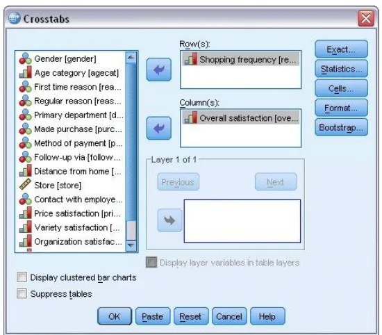
1. To run a Crosstabs analysis, from the menus choose: Analyze > Descriptive Statistics > Crosstabs...
Figure 44 Crosstabs dialog box
Figure 45 Statistics dialog box
6. Select Gamma, Somer's d, Kendall's tau-b, and Kendall's tau-c. 7. Click Continue.
8. Click OK in the Crosstabs dialog box.
4.2.2. Crosstabulation table
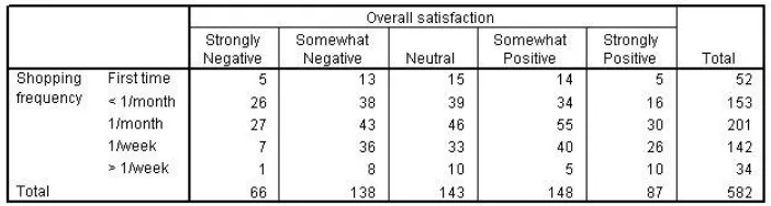
Figure 46 Crosstabulation for Shopping frequency by Overall satisfaction
The crosstabulation shows no clear pattern. If any exists, it may be that people who shop more often are more satisfied.
4.2.3. Symmetric and directional measures
Symmetric and directional measures of ordinal association are based on the idea of accounting for concordance versus discordance. Each pairwise comparison of cases is classified as one of the following.
column variable. Concordance implies a positive association between the row and column variables.
A pairwise comparison is considered discordant if the case with the larger value in the row variable has the smaller value in the column variable. Discordance implies a negative association between the row and column variables.
A pairwise comparison is considered tied on one variable if the two cases take the same value on the row variable, but different values on the column variable (or vice versa). Being tied on one variable implies a weakened association between the row and column variables.
A pairwise comparison is considered tied if the two cases take the same value on both the row and column variables. Being tied implies nothing about the association between the variables.
The measures differ in how they treat each type of comparison.
4.2.3.1. Symmetric and directional measures
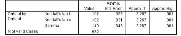
Figure 47 Symmetric measures for Shopping frequency by Overall satisfaction
Figure 48 Directional measures for Shopping frequency by Overall satisfaction
Gamma is P(concordant) - P(discordant), ignoring comparisons
Somer's d is a modification of gamma that accounts for
comparisons that are tied on one variable. Somer's d decreases with respect to gamma as the number of comparisons tied on one variable increases.
Tau-b also accounts for comparisons tied on one variable but does
not have a simple interpretation. It decreases with respect to gamma as the number of comparisons tied on one variable increases.
Tau-c also accounts for comparisons tied on one variable and does
not have a simple interpretation. Tau-cmay be preferable to tau-b when the numtau-bers of categories in the row and column variatau-bles are not equal.
The approximate significance value of each measure is equal to 0.001. Since this is less than 0.05, you can conclude there is a statistically significant relationship between Shopping frequency and Overall satisfaction. However, the value of each measure is less than 0.150, so while the relationship is different from 0, it is still rather weak.
4.2.4. Summary
Using Crosstabs' ordinal-by-ordinal measures, you have found a statistically significant, if not strong, positive association between Shopping frequency and Overall satisfaction. Given that there is a relationship, you may want to control for Shopping frequency in further analyses of customer satisfaction.
4.3. Using Crosstabs to measure the relative risk of an event
newspaper subscriptions, on the assumption that people who read newspapers are more likely to subscribe to magazines.
Use the Crosstabs procedure to test this theory by constructing a two-by-two table of Newspaper subscription byResponse and compute the relative risk that a person with a newspaper subscription will respond to the mailing. This information is collected in demo.sav. See the topic Sample Files for more information.
4.3.1. Running the analysis
1. To run a Crosstabs analysis, from the menus choose: Analyze > Descriptive Statistics > Crosstabs...
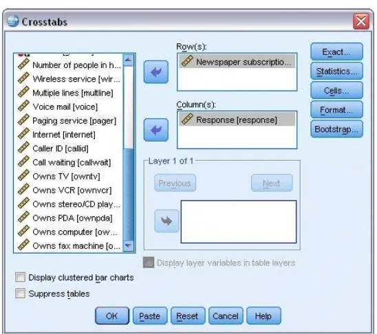
Figure 49 Crosstabs dialog box
2. Click Reset to restore the default settings.
3. Select Newspaper subscription as the row variable. 4. Select Response as the column variable.
Figure 50 Statistics dialog box
6. Select Risk. 7. Click Continue.
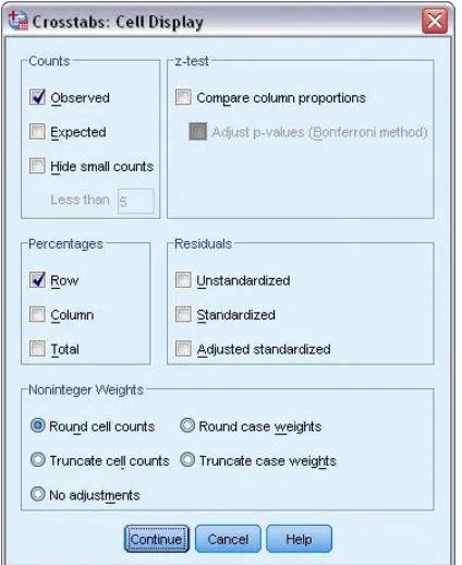
8. Click Cells in the Crosstabs dialog box. Figure 51 Cell Display dialog box
9. Select Row in the Percentages group. 10. Click Continue.
4.3.2. Crosstabulation
Figure 52 Crosstabulation for Newspaper subscription by Response
The crosstabulation shows that, overall, not very many people responded to the mailing. However, a greater proportion of newspaper subscribers responded.
4.3.3. Risk estimate
Figure 53 Risk estimate for Newspaper subscription by Response
subscriber responds to the mailing is 13.7%/86.3% = 0.158. Likewise, the estimate of the odds that a nonsubscriber responds is 8.2%/91.8% = 0.089. The estimate of the odds ratio is therefore 0.158/0.089 = 1.775. Note that the odds ratio is the ratio of the relative risk of responding, to the relative risk of not responding, or 1.668/0.940 = 1.775.
4.3.3.1. Odds ratio versus relative risk
Since it is a ratio of ratios, the odds ratio is very difficult to interpret. The relative risk is easier to interpret, so the odds ratio alone is not very helpful. However, there are certain commonly occurring situations in which the estimate of the relative risk is not very good and the odds ratio can be used to approximate the relative risk of the event of interest. The odds ratio should be used as an approximation to the relative risk of the event of interest when both of the following conditions are met:
The probability of the event of interest is small (<0.1). This condition guarantees that the odds ratio will make a good approximation to the relative risk. In this example, the event of interest is a response to the mailing.
The design of the study is case control. This condition signals that the usual estimate of the relative risk will likely not be good. A case-control study is retrospective, most often used when the event of interest is unlikely or when the design of a prospective experiment is impractical or unethical.
4.3.4. Adding income category as a layer variable
By targeting newspaper subscribers, you can increase the response rate to the mailings, but can you further target the mailings? Add Income category as a layer variable and test the homogeneity of the odds ratio to see if you obtain greater increases in the response rate.
4.3.4.1. Rerunning the analysis
Figure 54 Crosstabs dialog box
1. Recall the Crosstabs dialog box.
Figure 55 Statistics dialog box
4. Select Cochran's and Mantel-Haenszel statistics. 5. Click Continue.
6. Click OK in the Crosstabs dialog box.
4.3.4.2. Risk estimate
Figure 56 Risk estimate for Newspaper subscription by Response, controlling for Income category
indicates that you may be able to further target the mailings. To confirm that this relationship is not due to chance, see the tests of homogeneity of the odds ratio.
4.3.4.3. Tests of homogeneity of the odds ratio
Figure 57 Tests of homogeneity of the odds ratio for Newspaper subscription by Response, controlling for Income category
The Breslow-Day and Tarone's statistics test the homogeneity of the odds ratio across categories of the layer variable. The null hypothesis for these tests assumes that the odds ratio for Newspaper subscription by Response is equivalent for each value of Income category. The significance values are greater than 0.10, indicating that the odds ratio is in fact homogenous, which means that you should not use Income category to further target the mailings.
4.3.4.4. Tests of conditional independence
Figure 58 Tests of conditional independence for Newspaper subscription by Response, controlling for Income category
4.3.4.5. Mantel-Haenszel common odds ratio estimate
Figure 59 Mantel-Haenszel common odds ratio estimate for Newspaper subscription by Response, controlling for Income category response rate to direct mailings by targeting newspaper subscribers. Further, you found that the risk estimates were not constant across Income category, so you can increase your response rate even more by targeting lower-income newspaper subscribers.
4.4. Using Crosstabs to measure agreement
A company is interested in expanding its business, but has to choose from among 20 different sites to build. They have hired two consultants to separately evaluate these sites. In addition to an extended report, each consultant was asked to summarize each site as a good, fair, or poor prospect. You need to determine which sites the company should investigate further, and, if possible, determine which of the consultants the company should retain for further work.
4.4.1. Running the analysis
1. To run a Crosstabs analysis, from the menus choose: Analyze > Descriptive Statistics > Crosstabs...
Figure 60 Crosstabs dialog box
2. Click Reset to restore the default settings.
3. Select Rating from consultant 1 as the row variable. 4. Select Rating from consultant 2 as the column variable. 5. Click Statistics.
8. Click OK in the Crosstabs dialog box.
4.4.2. Kappa measure of agreement
Figure 62 Measure of agreement
The value of Kappa is statistically significantly different from 0, and its value of 0.429 suggests that the consultants' ratings are largely similar, with some exceptions.
4.4.3. Crosstabulation
Figure 63 Crosstabulation for Rating from consultant 1 by Rating from consultant
The crosstabulation reaffirms that the consultants largely agree. You can certainly remove the six sites they both considered Poor from consideration and perhaps ignore the five that were rated Poor by the second consultant andFair by the first. The four sites they rated as Good should be investigated and perhaps the two rated Good by the second consultant and Fair by the first. The two that both rated Fair may or may not be further examined, depending upon time and monetary constraints.
4.4.4. Summary
note that the valley in which the site is located is in the runoff path for snow thaw.
Further, the second consultant made more decisive ratings than the first, who rated rather conservatively. You decide to retain the second consultant for further work.
4.5. Comparing column proportions in Crosstabs
A human resources firm is analyzing the results of job satisfaction surveys and is interested in whether there is a relationship between the number of years an employee has been with their current employer and their level of job satisfaction.
Information from job satisfaction surveys for a set of employees is stored in demo.sav. See the topic Sample Filesfor more information. Use the Crosstabs procedure to examine the relationship, if any, between job satisfaction and years with current employer.
4.5.1. Running the analysis
1. To run a Crosstabs analysis, from the menus choose: Analyze > Descriptive Statistics > Crosstabs...
2. Select Years with current employer as the row variable. 3. Select Job satisfaction as the column variable.
4. Click Statistics.
Figure 65 Statistics dialog box
5. Select Chi-square. 6. Click Continue.
7. Click Cells in the Crosstabs dialog box. Figure 66 Cell Display dialog box
8. Deselect Observed.
p-The Compare column proportions option computes pairwise comparisons of column proportions and indicates which pairs of columns (for a given row) in the crosstabulation table are significantly different.
10. Click Continue.
11. Click OK in the Crosstabs dialog box.
4.5.2. Chi-square tests
Figure 67 Chi-square tests for Years with current employer by Job satisfaction
The chi-square test measures the discrepancy between the observed cell counts and what you would expect if the rows and columns were unrelated. The two-sided asymptotic significance of the chi-square statistic is 0, to the displayed precision. Since the significance value is clearly less than 0.05, you can conclude that there is a relationship between the number of years an employee has been with their current employer and their level of job satisfaction. To understand the nature of the relationship you need to examine the crosstabulation table, which includes the results of the column proportions tests.
4.5.3. Crosstabulation table with column proportions tests
Figure 68 Crosstabulation for Years with current employer by Job satisfaction
employer. For employees in the Less than 5 category, the percentages decrease with increased job satisfaction. To determine if the differences in those percentages, and thus the observed downward trend, are significant we'll examine the results of the column proportions tests.
satisfied categories are significantly different from each other as well as from the percentages in the other categories.
4.5.4. Summary