C H A P T E R
3
Groundwater Recharge
Neven Kresic
Alex Mikszewski
Woodard & Curran, Inc., Dedham, Massachusetts3.1 Introduction
Together with natural groundwater discharge and artificial extraction, groundwater recharge is the most important water budget component of a groundwater system. Un-derstanding and quantifying recharge processes are the prerequisites for any analysis of the resource sustainability. It also helps policymakers make better-informed decisions regarding land use and water management since protection of natural recharge areas is paramount to the sustainability of the groundwater resource. The first important step in recharge analysis is to consider the scale of the study area since the approach and methods of quantification are directly influenced by it. For example, it may be neces-sary to delineate and quantify local areas of focused recharge within several acres or tens of acres at a contaminated site where contaminants may be rapidly introduced into the subsurface. This scale of investigation would obviously not be feasible or needed for groundwater resources assessment in a large river basin (watershed). However, as illustrated further in this chapter, groundwater recharge is variable at all scales, in both space and time. It is, therefore, by default that any estimate of recharge involves aver-aging a number of quantitative parameters and their extrapolation-interpolation in time and space. This also means that there will always be a degree of uncertainty associated with quantitative estimates of recharge and that this uncertainty would also have to be analyzed and quantified. In other words, groundwater recharge is both a probabilistic and a deterministic process: if and when it rains (laws of probability), the infiltration of water into the subsurface and the eventual recharge of the water table will follow phys-ical (deterministic) laws. At the same time, both sets of laws (equations) use parameters that are either measured directly or estimated in some (preferably quantitative) way but would still have to be extrapolated-interpolated in space and time. For this reason, the quantification of groundwater recharge is one of the most difficult tasks in hydroge-ology. Unfortunately, this task is too often reduced to simply estimating a percentage of total annual precipitation that becomes groundwater recharge and then using that percentage as the “average recharge” rate for various calculations or groundwater mod-eling at all spatial and time scales. Following are some of the examples illustrating the
importance of not reducing the determination of recharge to a “simple,” nonconsequen-tial task.
r Recharge is often “calibrated” as part of groundwater modeling studies where
other model parameters and boundary conditions are considered to be more cer-tain (“better known”). In such cases, the model developer should clearly discuss uncertainties related to the “calibrated” recharge rates and the sensitivity of all key model parameters; a difference of 5 or 10 percent in aquifer recharge rate may not be all that sensitive compared to aquifer transmissivity (hydraulic con-ductivity) when matching field measurements of the hydraulic head; however, this difference is very significant in terms of aquifer water budget and analyses of aquifer sustainability.
r Recharge rate has implications on the shape and transport characteristics of
groundwater contaminant plumes. More or less direct recharge from land sur-face may result in a more or less diving plume, respectively. Different recharge rates also result in different overall concentrations—higher recharge results in lower concentrations (assuming that the incoming water is not contaminated).
r Rainwater that successfully infiltrates into the subsurface and percolates past the
root zone may take tens, or even hundreds, of years to traverse the vadose zone and reach the water table. The effects of recharge reduction are thus abstract, as groundwater users do not face immediate consequences. As a result, land use changes are often made without consideration of impacts to groundwater recharge.
r Natural and anthropogenic climate changes also alter groundwater recharge
patterns, the effects of which will be faced by future generations.
As discussed earlier in Chap. 2, water budget and groundwater recharge terms are often used interchangeably, sometimes causing confusion. In general, infiltration refers to any water movement from the land surface into the subsurface. This water is called potential recharge, indicating that only a portion of it may eventually reach water table (saturated zone). The term “actual recharge” is being increasingly used to avoid any possible confusion: it is the portion of infiltrated water that reaches the aquifer, and it is confirmed based on groundwater studies. The most obvious confirmation that actual groundwater recharge is taking place is rise in water table elevation (hydraulic head). However, the water table can also rise because of cessation of groundwater extraction (pumping), and this possibility should always be considered. Effective infiltration and deep percolation refer to water movement below the root zone and are often used to approximate actual recharge. Since evapotranspiration (ET) (loss of water to the atmo-sphere) refers to water at both the surface and subsurface, this should be clearly indicated.
3.2 Rainfall-Runoff-Recharge Relationship
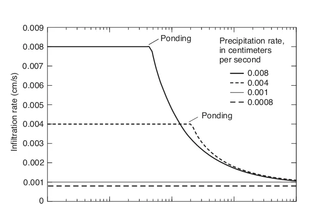
subtracting what is lost to overland flow (runoff) and evapotranspiration (ET). The key to the rainfall-runoff relationship is the soil type, the antecedent moisture condition, and the land cover. Soils that are well drained generally have high effective porosities and high hydraulic conductivities, whereas soils that are poorly drained have higher total porosities and lower hydraulic conductivities. These physical properties combine with initial moisture content to determine the infiltration capacity of surficial soils. Wet, poorly drained soils will readily produce runoff, while dry, well-drained soils will readily absorb rainfall. Land cover determines the fraction of precipitation available for infiltration. Impervious, paved surface prevent any water from entering the soil column, while open, well-vegetated fields are conducive to infiltration. Regardless of soil type, antecedent moisture, or land cover, the chain of events occurring during a storm event is the same. Available rainfall will infiltrate the subsurface until the rate of precipitation exceeds the infiltration capacity of the soil, at which point ponding and subsequent runoff will occur. Runoff either collects in discrete drainage channels or moves as overland sheet flow. It is important to understand that infiltration continues throughout the storm event, even as runoff is being produced. The infiltration rate after ponding begins to decrease and asymptotically approaches the saturated hydraulic conductivity of the soil media. Figure 3.1 illustrates typical infiltration patterns for four different rainfall events for the same soil with the saturated hydraulic conductivity of about 0.001 cm/s.
Simple calculations of runoff and water retention volumes in a watershed are possible using the U.S. Department of Agriculture Soil Conservation Service (SCS) runoff curve number (CN) method, updated in Technical Release 55 (TR-55) of the U.S. Department of Agriculture (USDA, 1986). TR-55 presents simplified procedures for estimating direct surface runoff and peak discharges in small watersheds. While it gives special emphasis to urban and urbanizing watersheds, the procedures apply to any small watershed in which certain limitations (assumptions) are met. Hydrologic studies to determine runoff
0.008
10 100 1000 10,000 100,000
Time since start of infiltration (s)
Inf
and peak discharge should ideally be based on long-term stationary streamflow records for the area. Such records are seldom available for small drainage areas. Even where they are available, accurate statistical analysis of them is often impossible because of the conversion of land to urban uses during the period of record. It, therefore, is necessary to estimate peak discharges with hydrologic models based on measurable watershed characteristics (USDA, 1986).
In TR-55, runoff is determined primarily by amount of precipitation and by infiltration characteristics related to soil type, soil moisture, antecedent rainfall, cover type, impervi-ous surfaces, and surface retention. Travel time is determined primarily by slope, length of flow path, depth of flow, and roughness of flow surfaces. Peak discharges are based on the relationship of these parameters and on the total drainage area of the watershed, the location of the development, the effect of any flood control works or other natural or manmade storage, and the time distribution of rainfall during a given storm event.
The model described in TR-55 begins with a rainfall amount uniformly imposed on the watershed over a specified time distribution. Mass rainfall is converted to mass runoff by using a runoff CN. Selection of the appropriate CN depends on soil type, plant cover, amount of impervious areas, interception, and surface storage. Runoff is then transformed into a hydrograph by using unit hydrograph theory and routing procedures that depend on runoff travel time through segments of the watershed (USDA, 1986). As pointed out by the authors, to save time, the procedures in TR-55 are simplified by assumptions about some parameters. These simplifications, however, limit the use of the procedures and can provide results that are less accurate than more detailed methods. The user should examine the sensitivity of the analysis being conducted to a variation of the peak discharge or hydrograph.
The SCS runoff equation is
Q= (P−Ia)
2
(P−Ia)+S (3.1)
whereQ=runoff (in) P=rainfall (in)
S=potential maximum retention after runoff begins (in) Ia=initial abstraction (in)
Initial abstraction is all losses before runoff begins. It includes water retained in surface depressions and water intercepted by vegetation, evaporation, and infiltration. Iais highly variable but generally is correlated with soil and cover parameters. Through
studies of many small agricultural watersheds,Iawas found to be approximated by the
following empirical equation:
Ia=0.2S (3.2)
By removingIaas an independent parameter, this approximation allows use of a
com-bination ofSand Pto produce a unique runoff amount. Substituting Eq. (3.2) into Eq. (3.1) gives
Q= (P−0.2S)
2
Direct runoff (
FIGURE3.2 Solution of runoff equation. Curves are for conditionIa= 0.2Sand Eq. (3.3). (From USDA, 1986.)
Water retentionS, which includes infiltration, interception by vegetation, ET, and storage in surface depressions, is calculated using the CN approach, taking into account antecedent soil moisture, soil permeability, and land cover. It is related to CN through the equation:
S=1000
CN −10 (3.4)
CNs for watershed range from 0 to 100, with 100 being perfectly impervious. The graph in Fig. 3.2 solves Eqs. (3.2) and (3.4) for a range of CNs and rainfall events. Table 3.1 is an example of CNs for several types of agricultural land cover that can be selected based on available information. TR-55 also includes tables for various other land covers. Soils are classified into four hydrologic soil groups (A, B, C, and D) according to their minimum infiltration rate, which is obtained for bare soil after prolonged wetting. Appendix A in TR-55 defines the four groups and provides a list of most of the soils in the United States and their group classification. The hydrologic characteristics of the four groups are as follows (Rawls et al., 1993):
r Group A soils have low runoff potential and high infiltration rates even when
thoroughly wetted. They consist mainly of deep, well to excessively drained sands or gravels. The USDA soil textures normally included in this group are sand, loamy sand, and sandy loam. These soils have infiltration rate greater than 0.76 cm/h.
r Group B soils have moderate infiltration rates when thoroughly wetted and
Curve Numbers for Hydrologic Soil Group
Hydrologic
Cover Type Condition A B C D
Pasture, grassland, or range-continuous Poor 68 79 86 89
forage for grazing1 Fair 49 69 79 84
Good 39 61 74 80
Meadow—continous grass, protected from grazing, generally moved for hay
30 58 71 78
Brush—brush-weed-grass mixture with Poor 48 67 77 83
brush the major element2 Fair 35 56 70 77
Good 303 48 65 73
Woods-grass combination (orchard or Poor 57 73 82 86
tree farm)4 Fair 43 65 76 82
Good 32 58 72 79
Woods5 Poor 45 66 77 83
Fair 36 60 73 79
Good 303 55 70 77
1Poor:<50% ground cover or heavily gazed with no mulch;fair: 50–75% ground cover and not heavily gazed;good:>75% ground cover and lightly or only occasionaly grazed.
2Poor: <50% ground cover;fair: 50–75% ground cover;good:>75% ground cover. 3Actual curve number is less than 30; use CN=30 for runoff computations. 4Computed for areas with 50% woods and 50% grass (pasture) cover.
5Poor: Forest litter, small trees, and brush are destroyed by heavy grazing or regular burning;fair: woods are grazed but not burned, and some forest litter covers the soil;good: woods are protected from grazing, and litter and brush adequately cover the soil.
From USDA, 1986.
TABLE3.1 Runoff Curve Numbers for Selected Agricultural Lands, for Average Runoff Condition andIa=0.2S.
well-drained soils having moderately fine to moderately coarse textures. The USDA soil textures normally included in this group are silt loam and loam. These soils have an infiltration rate between 0.38 and 0.76 cm/h.
r Group C soils have low infiltration rates when thoroughly wetted and consist
mainly of soils with a layer that impedes downward movement of water and soils with moderately fine to fine texture. The USDA soil texture normally included in this group is sandy clay loam. These soils have an infiltration rate between 0.13 and 0.38 cm/h.
r Group D soils have high runoff potential. They have very low infiltration rates
Watersheds with higher CNs generate more runoff and less infiltration. Examples in-clude watersheds with high proportion of paved, impervious surfaces. Dense forestland and grasslands have the lowest CNs and retain high proportions of rainfall. However, it is important to understand that most urban areas are only partially covered by impervi-ous surfaces; the soil remains an important factor in runoff estimates. Urbanization has a greater effect on runoff in watersheds with soils having high infiltration rates (sands and gravels) than in watersheds predominantly of silts and clays, which generally have low infiltration rates (USDA, 1986).
TR-55 includes tables and graphs for selection of all quantitative parameters needed to select CNs and calculate runoff for thousands of soil types and land covers in the United States. Representative land covers include bare land, pasture, western desert urban area, and woods to name a few. The soils in the area of interest may be identified from a soil survey report, which can be obtained from local SCS offices or soil and water conservation district offices.
While the SCS method enables calculation of runoff, it does not provide for exact estimation of infiltration, which is only one of the calculated overall water retention components. The calculated volume of water retained by the watershed includes terms for ET and interception by vegetation. Knowledge of the vegetative conditions of the watershed in question will help determine the distribution of rainfall retention. Vege-tative interception will be more significant for a forested area than for an open field. One must also remember that runoff-producing storm events allow infiltration rates to asymptotically approach the saturated hydraulic conductivity of surficial soils. Knowl-edge of the physical properties of watershed soils is, therefore, necessary for estimation of infiltration rates.
3.3 Evapotranspiration
ET is often the second largest component of the water budget, next to precipitation. Ap-proximately 65 percent of all precipitation falling on landmass returns to the atmosphere through ET, which can be defined as the rate of liquid water transformation to vapor from open water, bare soil, or vegetation with soil beneath (Shuttleworth, 1993). Tran-spiration is defined as the fraction of total ET that enters the atmosphere from the soil through the plants. The rate of ET, expressed in inches per day or millimeters per day, has traditionally been estimated using meteorological data from climate stations located at particular points within a region and parameters describing transpiration by certain types of vegetation (crop). There are two standard rates used as estimates of ET:potential evaporationandreference crop evaporation.
Potential evaporationE0is the quantity of water evaporated per unit area, per unit
time from an idealized, extensive free water surface under existing atmospheric condi-tions. This is a conceptual entity that measures the meteorological control on evaporation from an open water surface. E0 is commonly estimated from direct measurements of
evaporation with evaporation pans (Shuttleworth, 1993). Note thatE0is also called
po-tential evapotranspiration (PET), even though as defined it does not involve plant activity. Reference crop evapotranspiration Ec is the rate of evaporation from an idealized
grass crop with a fixed crop height of 0.12 m, an albedo of 0.23, and a surface resistance of 69 s·m−1(Shuttleworth, 1993). This crop is represented by an extensive surface of short
and not short of water. When estimating actual ET from a vegetated surface it is common practice to first estimateEcand then multiply this rate by an additional complex factor
called the crop coefficientKc.
There are many proposed and often rather complex empirical equations for estimating E0andEc, using various parameters such as air temperature, solar radiation, radiation
exchange for free water surface, hours of sunshine, wind speed, vapor pressure deficit (VPD), relative humidity, and aerodynamic roughness (for example, see Singh, 1993; Shuttleworth, 1993; Dingman, 1994). The main problem in applying empirical equations to a very complex physical process such as ET is that in most cases such equations produce very different results for the same set of input parameters. As pointed out by Brown (2000), even in cases of the most widely used group of equations referred to as “modified Penman equations,” the results may vary significantly (Penman proposed his equation in 1948, and it has been modified by various authors ever since).
The PET from an area can be estimated from the free water evaporation assuming that the supply of water to the plant is not limited. Actual evapotranspirationEactequals
the potential value,E0as limited by the available moisture (Thornthwaite, 1946). On a
natural watershed with many vegetal species, it is reasonable to assume that ET rates do vary with soil moisture since shallow-rooted species will cease to transpire before deeper-rooted species (Linsley and Franzini, 1979). A moisture-accounting procedure can be established by using the continuity equation:
P−R−G0−Eact=M (3.5)
where P=precipitation R=surface runoff G0=subsurface outflow
Eact=actual ET
M=the change in moisture storage Eactis estimated as
Eact=E0
Mact
Mmax
(3.6) whereMact=computed soil moisture stage on any date andMmax=assumed maximum
soil moisture content (Kohler, 1958, from Linsley and Franzini, 1979).
In addition to available soil moisture, plant type is another important component of actual ET, as certain species require more water than others. A Colorado State University study in eastern Colorado examined the water requirements of different crops in 12 agri-cultural areas (Broner and Schneekloth, 2007). On average, corn required 24.6 in/season, sorghum required 20.5 in/season, and winter wheat required 17.5 in/season. Allen et al. (1998) present detailed guidelines for computing crop water requirements together with representative values for various crops. Native vegetation to semiarid and arid en-vironments is more adept at surviving in low-moisture soils and generates much lower Eactvalues than introduced species.Eactincreases with increasing plant size and canopy
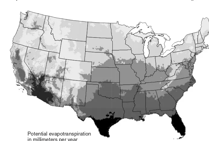
VPD, a measure of the “drying power” of the atmosphere. The VPD quantifies the gradi-ent in water vapor concgradi-entration between vegetation and the atmosphere and increases with increasing temperature and decreasing humidity (Brown, 2000). A less publicized factor influencing open soil evaporation is soil type. Open soil evaporation occurs in two phases: a rapid phase involving capillary conduction followed by a long-term, energy-intensive phase involving vapor diffusion. Initial evaporation rates from coarse-grained soils are therefore very high, as these soils have high conductivities. However, over time, fine-grained soils with high porosities yield greater evaporation quantities because of greater long-term water retention (Wythers et al., 1999). In other words, the conductive phase lasts much longer for fine-grained soils than coarse-grained soils. Yet for either soil type, extended dry periods will lead to desiccation of soils through vapor diffusion. Figure 3.3 shows regional PET patterns across the continental United States, demon-strating the significance of the above contributing factors. The highest PET values are found in areas of high temperatures and low humidity, such as the deserts of southeastern California, southwestern Arizona, and southern Texas (Healy et al., 2007). Mountainous regions exhibit low PET values because of colder temperatures and the prevalence of moist air. It is interesting that southern Florida has remarkably high PET rates rivaling those in desert environments. This may be attributable to the dense vegetative cover of the subtropical Florida landscape, or the more seasonal trends in annual precipitation (i.e., more defined rainy and dry seasons).
A very detailed study of ET rates by vegetation in the spring-fed riparian areas of Death Valley, United States, was performed by the U.S. Geological Survey (USGS). The study was initiated to better quantify the amount of groundwater being discharged annually from these sensitive areas and to establish a basis for estimating water rights
0–564 565–709
710–877 878–1,074
1,075–1,662 Potential evapotranspiration
in millimeters per year
and assessing future changes in groundwater discharge in the park (Laczniak et al., 2006). ET was estimated volumetrically as the product of ET-unit (general vegetation type) acreage and a representative ET rate. ET-unit acreage was determined from high-resolution multispectral imagery. A representative ET rate was computed from data collected in the Grapevine Springs area using the Bowen ratio solution to the energy budget or from rates given in other ET studies in the Death Valley area. The groundwater component of ET was computed by removing the local precipitation component from the ET rate.
Figure 3.4 shows instrumentation used to collect data for the ET computations at the Grapevine Springs site. The instruments included paired temperature and humidity probes, multiple soil heat-flux plates, multiple soil temperature and moisture probes, a net radiometer, and bulk rain gauge. In addition, a pressure sensor was set in a nearby
Net radiometer
A S O N D J F M A M J J A S O N D J F M A M J J A S O N D
2000 2001 Water Year 2002 2003
Day number referenced to January 1, 2000
300 400 500 600 700 800 900 1,000 1,100
Daily evapotranspiration (in.)
FIGURE3.5 Daily evapotranspiration and mean daily groundwater level at Grapevine Springs ET site, from September 28, 2000, to November 3, 2002 (day numbers 272 and 1038, respectively). (From Laczniak et al., 2006.)
shallow well to acquire information on the daily and annual water table fluctuation. Micrometeorologic data were collected at 20-min intervals and water levels were collected at hourly intervals (Laczniak et al., 2006).
The results of the study show that ET at the Grapevine Springs site generally begins increasing in late spring and peaks in the early through midsummer period (June and July). During this peak period, daily ET ranged from about 0.18 to 0.25 in (Fig. 3.5) and monthly ET ranged from about 5.7 to 6.2 in. ET totaled about 2.7 ft in water year 2001 and about 2.3 ft in water year 2002. The difference in precipitation between the two water years is nearly equivalent to the difference in annual ET. Annual trends in daily ET show an inverse relation with water levels—as ET begins increasing in April, water levels begin declining, and as ET begins decreasing in September, water levels begin rising. The slightly greater ET and higher water levels in water year 2001, compared with water year 2002, are assumed to be a response to greater precipitation.
The groundwater component of ET at the Grapevine Springs ET site ranged from 2.1 to 2.3 ft, with the mean annual groundwater ET from high-density vegetation being 2.2 ft (Laczniak et al., 2006).
3.4 Infiltration and Water Movement Through Vadose Zone
which water is transmitted downward through the soil. Thus, soil surface conditions alone cannot increase infiltration unless the transmission capacity of the soil profile is adequate. Under conditions where the surface entry rate (rainfall intensity) is slower than the transmission rate of the soil profile, the infiltration rate will be limited by the rainfall intensity (water supply). Until the top soil horizon is saturated (i.e., the soil moisture deficit is satisfied), the infiltration rate will be constant, as shown in Fig. 3.1. For higher rainfall intensities, all the rain will infiltrate into the soil initially until the soil surface becomes saturated (θ =θs,h≥0,z=0), that is, until the so-calledponding time (tp) is
reached. At that point, the infiltration is less than the rainfall intensity (approximately equal to the saturated hydraulic conductivity of the media) and surface runoff begins. These two conditions are expressed as follows (Rawls et al., 1993):
−K(h)∂h
∂z +1=R θ(0,t)≤θs t≤tp (3.7)
h=h0 θ(0,t)=θs t≥tp (3.8)
whereK(h)=hydraulic conductivity for given soil water potential (degree of saturation)
h =soil water potential
h0 =small positive ponding depth on the soil surface
θ =volumetric water content
θs =volumetric water content at saturation
z=depth from land surface
tp =time from the beginning of rainfall until ponding starts (ponding time)
R=rainfall intensity
The transmission rates can vary at different horizons in the unsaturated soil profile. After saturation of the uppermost horizon, the infiltration rate is limited to the lowest transmission rate encountered by the infiltrating water as it travels downward through the soil profile. As water infiltrates through successive soil horizons and fills in the pore space, the available storage capacity of the soil will decrease. The storage capacity available in any horizon is a function of the porosity, horizon thickness, and the amount of moisture already present. Total porosity and the size and arrangement of the pores have significant effect on the availability of storage. During the early stage of a storm, the infiltration process will be largely affected by the continuity, size, and volume of the larger-than-capillary (“noncapillary”) pores, because such pores provide relatively little resistance to the infiltrating water. If the infiltration rate is controlled by the transmission rate through a retardant layer of the soil profile, then the infiltration rate, as the storm progresses, will decrease as a function of the decreasing storage availability above the restrictive layer. The infiltration rate will then equal the transmission rate through this restrictive layer until another, more restrictive, layer is encountered by the water (King, 1992). The soil infiltration capacity decreases in time and eventually asymptotically reaches the value of overall saturated hydraulic conductivity Ks of the affected soil
column as illustrated in Fig. 3.1.
in relatively small quantities, may dramatically reduce infiltration rate as they become wet and swell. Runoff conditions on soils of low permeability develop much sooner and more often than on uniform, coarse sands and gravels, which have infiltration rates higher than most rainfall intensities.
The soil surface can become encrusted with, or sealed by, the accumulation of fines or other arrangements of particles that prevent or retard the entry of water into the soil. As rainfall starts, the fines accumulated on bare soil may coagulate and strengthen the crust, or enter soil pores and effectively seal them off. A soil may have excellent subsurface drainage characteristics but still have a low infiltration rate because of the retardant effect of surface crusting or sealing (King, 1992).
3.4.1
Soil Water Retention and Hydraulic Conductivity
Similar to groundwater flow in the saturated zone, the flow of water in the unsaturated zone is governed by two main parameters—the change in total potential (hydraulic head) along the flow path between the land surface and the water table and the hydraulic conductivity of the soil media. However, both parameters depend on the volumetric water content in the porous medium; they change in time and space as the soil becomes more or less saturated in response to water input and output such as infiltration and ET. Air that fills pores unoccupied by water in the vadose zone exerts an upward suction effect on water caused by capillary and adhesive forces. This suction pressure of the soil, also calledmatric potential, is lower than the atmospheric pressure. It is the main characteristic of the vadose zone governing water movement from the land surface to the water table. The water-retention characteristic of the soil describes the soil’s ability to store and release water and is defined as the relationship between the soil water content and the matric potential. The water-retention characteristic is also known as moisture characteristic curve, which when plotted on a graph shows water content at various depths below ground surface versus matric potential (Fig. 3.6). Again, the matric potential is always negative above the water table, since the suction pressure is lower than the atmospheric pressure. The matric potential is a function of both the water content and the sediment texture: it is stronger in less saturated and finer soils. As the soil saturation increases, the matric potential becomes “less negative.” At the water table, the matric potential is zero and equals the atmospheric pressure. Other terms that are synonymous with matric potential but may differ in sign or units are soil water suction, capillary potential, capillary pressure head, suction head, matric pressure head, tension, and pressure potential (Rawls et al., 1993).
As the moisture content increases, suction pressure decreases, causing a correspond-ing increase in hydraulic conductivity. As a result, soils with high antecedent moisture contents will support a greater long-term drainage rate than dry soils. At saturation (i.e., at and immediately above the water table in the capillary fringe), the hydraulic conduc-tivity of the soil media is equal to the saturated hydraulic conducconduc-tivity. Figure 3.7 shows unsaturated hydraulic conductivity as the function of matric potential for the same two soil types shown in Fig. 3.6.
3.4.2
Darcy’s Law
0.1 0.2 0.3 -200
-150
-100
-50
0
S
ucti
o
n
head
(c
m
)
0
Saturation
0.4 0.5 0.6 0.7 0.8 0.9 1
Fine sand
Coarse sand
FIGURE3.6 Two characteristic moisture curves for fine and coarse sand.
Fine sand
Coarse sand
Relative hydraulic conductivity (dimensionless) 0
-20 -40 -60 -80
Sucti
on
head
(c
m
)
-100 -120 -140 -160 -180 -200
0 0.1 0.2 0.3 0.4 0.5 0.6 0.7 0.8 0.9 1
Darcy-Buckingham equation) is
q= −K()∂H
∂z = −K(θ) ∂
∂z(+z) (3.9)
where q =flow per unit width
K()=unsaturated hydraulic conductivity given as function of matric potential θ =soil moisture content
H=total water potential z=elevation potential
=matric potential or pressure head
The matric and elevation potentials (heads) combine to form the total water potential (head). Pressure head is negative in the unsaturated zone (causing the “suction” effect), zero at the water table, and positive in the saturated zone. As in the saturated zone, water in the vadose zone moves from large to small water potentials (heads).
For deep vadose zones common to the American West, soil hydraulic properties can be used to simply calculate recharge flux using Darcy’s law. The underlying assumption of the “Darcian method” is that moisture content becomes constant at some depth, such that there is no variation in matric potential or pressure headhwith depthzand that all drainage is due to gravity alone (see Fig. 3.8). Under these conditions, the deep drainage rate is approximately equal to the measured unsaturated hydraulic conductivity (Nimmo et al., 2002). The equations describing this relationship are the following:
q= −K()
d dz +1
d
dz ≈0 (3.10)
q≈ −K()
Moisture content, dimensionless
0.20 0.25 0.30 0.35 0.40
6
8
Depth (m)
4 2 0
Winter Spring Summer Fall
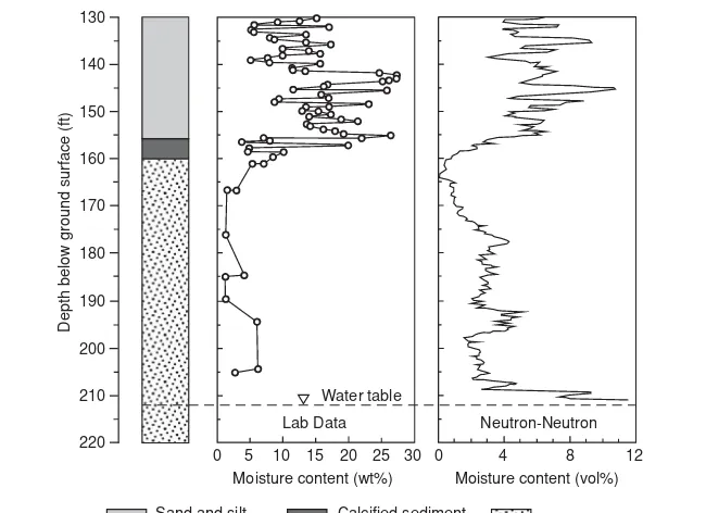
0 5 10 15 20 25 30 0 4 8 12 Moisture content (vol%) Moisture content (wt%)
220 210 200 190 180 170 160 150 140 130
Water table
Neutron-Neutron Lab Data
Depth below ground surface (ft)
Sandy gravel Calcified sediment
(caliche) Sand and silt
(mud)
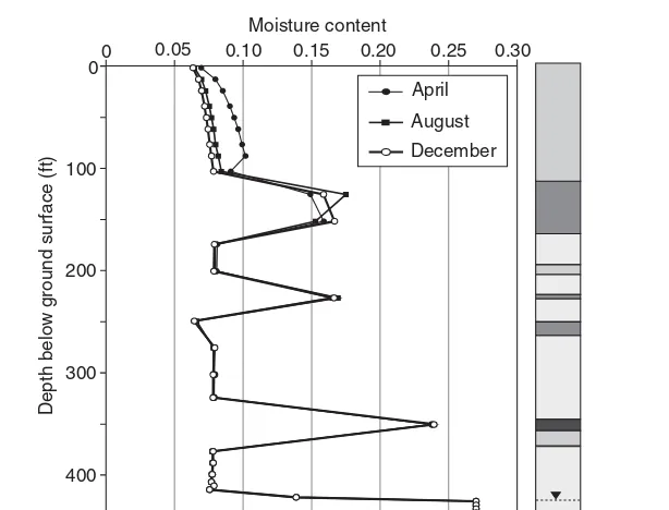
FIGURE3.9 Lithology and moisture distribution as a function of depth within a borehole in a deep vadose zone. (Modified from Serne et al., 2002.)
Alternatively, knowledge of matric potential (pressure head) at different depths enables direct calculation of recharge flux from the above equation. Velocity of the recharge front can be calculated by dividing the flux by soil moisture content.
Darcy’s law illustrates the complexity of unsaturated flow, as both hydraulic con-ductivity and pressure head are functions of the soil moisture content (θ). Another crucial factor influencing drainage rates is vadose zone lithology. Deep vadose zones often have a high degree of heterogeneity, created by distinct depositional periods. This limits the application of Eq. (3.10). For example, layers of fine-grained clays and silts are common to deep basins of the American West. As a result, moisture perco-lating through the vadose zone often encounters low permeability strata, including calcified sediment layers as shown in Fig. 3.9. Presence of low-permeable intervals in the vadose zone greatly delays downward migration and may cause significant lateral spreading. Therefore, the time lag for groundwater recharge may be on the order of hundreds of years or more for deep vadose zones with fine-grained sediments. Fur-thermore, moisture is lost to lateral spreading and storage. Detailed lithologic charac-terization of the vadose zone is essential in quantification of groundwater recharge as well as in planning and designing artificial recharge systems. Knowledge of site-specific geology is also helpful in qualitatively understanding the time scale of vadose zone processes.
3.4.3
Equations of Richards, Brooks and Corey, and van Genuchten
Water flow in variably saturated soils is traditionally described with the Richards equa-tion (Richards, 1931) as follows (van Genuchten et al., 1991):
C∂h ∂t =
∂ ∂z
K∂h ∂z −K
(3.11)
where h =soil water pressure head or matric potential (with dimensionL) t=time (T)
z=soil depth (L)
K =hydraulic conductivity (LT−1)
C =soil water capacity (L−1) approximated by the slopedθ/dhof the soil water
retention curveθ(h), in whichθis the volumetric water content (L3L−1).
Equation (3.11) may also be expressed in terms of the water content if the soil profile is homogeneous and unsaturated (h≤0):
∂θ ∂t =
∂ ∂z
D∂θ ∂z−K
(3.12)
whereD=soil diffusivity (L2T−1) defined as
D=Kdh
dθ (3.13)
The unsaturated soil hydraulic functions in the above equations are the soil water retention curve,θ(h), the hydraulic conductivity function,K(h) orK(θ), and the soil water diffusivity functionD(θ). Several functions have been proposed to empirically describe the soil water retention curve. One of the most widely used is the equation of Brooks and Corey (van Genuchten et al., 1991; ˇSimnek et al., 1999):
θ=
θr+(θs−θr)(αh)−λ (h<−1/α)
θs (h≥ −1/α)
(3.14)
where θ =volumetric water content θr=residual water content
θs =saturated water content
α=an empirical parameter (L−1) whose inverse (1/α) is often referred to as the
air entry value or bubbling pressure α=a negative value for unsaturated soils
λ=a pore-size distribution parameter affecting the slope of the retention function
Equation (3.14) may be written in a dimensionless form as follows:
Se=
(αh)−λ (h<−1/α)
1 (h≥ −1/α) (3.15)
whereSe=effective degree of saturation, also called the reduced water content (0<Se<
1):
Se=
θ−θr
θs−θr
(3.16)
The residual water contentθrin Eq. (3.16) specifies the maximum amount of water in
a soil that will not contribute to liquid flow because of blockage from the flow paths or strong adsorption onto the solid phase (Luckner et al., 1989, from van Genuchten et al., 1991). Formally,θrmay be defined as the water content at which bothdθ/dhandK reach
zero whenh becomes large. The residual water content is an extrapolated parameter and may not necessarily represent the smallest possible water content in a soil. This is especially true for arid regions where vapor phase transport may dry out soils to water contents well belowθr. The saturated water contentθsdenotes the maximum volumetric water content of a soil. The saturated water content should not be equated to the porosity of soils;θsof field soils is generally about 5 to 10 percent smaller than the porosity because of entrapped or dissolved air (van Genuchten et al., 1991).
The Brooks and Corey equation has been shown to produce relatively accurate results for many coarse-textured soils characterized by relatively uniform pore- or particle-size distributions. Results have generally been less accurate for many fine-textured and undisturbed field soils because of the absence of a well-defined air-entry value for these soils. A continuously differentiable (smooth) equation proposed by van Genuchten (1980) significantly improves the description of soil water retention:
Se=
1
[1+(αh)n]m (3.17)
whereα,n, andm are empirical constants affecting the shape of the retention curve (m=1−1/n). By varying the three constants, it is possible to fit almost any measured field curve. It is this flexibility that made the van Genuchten equation arguably the most widely used in various computer models of unsaturated flow and contaminant fate and transport. Combining Eqs. (3.16) and (3.17) gives the following form of the van Genuchten equation:
θ(h)=θr+ θs−θr
[1+(αh)n]1−n1 (3.18)
the following form (van Genuchten et al., 1991):
K(Se)=KsSe
f(Se)
f(l)
2
(3.19)
f(Se)=
Se
0
1
h(x)d x (3.20)
where Seis given by Eq. (3.16) Ks=hydraulic conductivity at saturation, andl=an
empirical pore-connectivity (tortuosity) parameter estimated by Mualem to be about 0.5 as an average for many soils.
Detailed solution of the Mualem’s model by incorporating Eq. (3.17) is given by van Genuchten et al. (1991). This solution, sometimes called van Genuchten-Mualem equation, has the following form:
K(Se)=KoSel
1−
1−Sn/(n−1)
e
1−1
n
2
(3.21)
whereKois the matching point at saturation, a parameter often similar, but not necessarily
equal, to the saturated hydraulic conductivity (Ks). Fitting the van Genuchten-Mualem
equation to soil data gives good results in most cases. It is important to note that the curve-fit parameters and those representing matching-point saturation and tortuosity tend to lose physical significance when fit to laboratory data. Hence, one must remember that these terms are best described as mathematical constants rather than physical properties of the soils in question.
Rosetta (Schaap, 1999) and RETC (van Genuchten et al., 1991) are two very useful public domain programs developed at the U.S. Salinity Laboratory for estimating unsatu-rated zone hydraulic parameters required by the Richards and van Genuchten equations. The programs provide models of varying complexity, starting with simple ones such as percentages of sand, silt, and clay in the soil and ending with rather complex options where laboratory data are used to fit unknown hydraulic coefficients.
3.5 Factors Influencing Groundwater Recharge
3.5.1
Climate
climatic types based on the average annual variations of precipitation, PET, and the consequent soil moisture deficit or surplus. Soil water balance models, which are very similar to the soil moisture model for classifying worldwide climate, have been devel-oped to estimate recharge. These models utilize more specific data, such as soil type and moisture-holding capacity, vegetation type and density, surface-runoff characteristics, and spatial and temporal variations in precipitation. Various soil water balance models used in estimating recharge in arid and semiarid regions of the world are discussed by Bedinger (1987), who includes an annotated bibliography of 29 references. The estimated recharge rates have wide scatter, which is attributed to differences in applied methods, real differences in rates of infiltration to various depths and net recharge, and varying characteristics of soil types, vegetation, precipitation, and climatic regime.
Based on a detailed study of a wide area in the mid-continental United States span-ning six states, Dugan and Peckenpaugh (1985) concluded that both the magnitude and the proportion of potential recharge from precipitation decline as the total precipitation declines (see Fig. 3.10), although other factors including climatic conditions, vegetation, and soil type also affect potential recharge. The limited scatter among the points in Fig. 3.10 indicates a close relationship between precipitation and recharge. Furthermore, the relationship becomes approximately linear where mean annual precipitation exceeds 30 in and recharge exceeds 3 in. Presumably, when the precipitation and recharge are less than these values, disproportionably more infiltrating water is spent on satisfying the moisture deficit in dry soils. The extremely low recharge in the western part of the study area, particularly Colorado and New Mexico, appears to be closely related to the high PET found in these regions. Seasonal distribution of precipitation also shows a strong relationship to recharge. Areas of high cool-season precipitation tend to receive higher amounts of recharge. Where PET is low and long winters prevail, particularly in the Nebraska and South Dakota parts of the study area, effectiveness of cool-season precipi-tation as a source of recharge increases. Overall, however, when cool-season precipiprecipi-tation is less than 5 in, recharge is minimal. Dugan and Peckenpaugh (1985) conclude that gen-eralized patterns of potential recharge are determined mainly by climatic conditions.
10 20 30 40 50
15 10
5 0
Recharge (in.)
Precipitation (in.)
MOUNTAIN BLOCK BASIN
Riparian Zone
Mountain Front Zone
Local Flow Paths
Regional Flow Paths
FIGURE3.11 Schematic of mountain block contribution to recharge of a groundwater system. (From Wilson and Guan, 2004; copyright American Geophysical Union.)
Smaller variations within local areas, however, are related to differences in land cover, soil types, and topography.
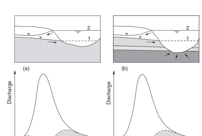
A large portion of groundwater recharge is derived from winter snowpack, which provides a slow, steady source of infiltration. Topographically, higher elevations typically receive more precipitation, including snow, than valleys or basins. Coupled with low PET, they produce ideal recharge conditions. This fact is especially important in areas such as the Basin and Range province of the United States where the so-called mountain block recharge (MBR) is critical component of a groundwater system water balance (Fig. 3.11; Wilson and Guan, 2004). High-elevation recharge produces the confined aquifer condi-tions that millions of people rely on for potable water. Snowmelt recharge in mountain ranges occurs in a cyclical pattern, described as follows (Flint and Flint, 2006):
r During daytime, snowmelt infiltrates thin surface soils and migrates down to
the soil-bedrock interface.
r The soil-bedrock interface becomes saturated, and once the infiltration rate
ex-ceeds the bulk permeability of the bedrock matrix, moisture enters the bedrock fracture system.
r At night, snow at the ground surface refreezes while stored moisture in surface
soils drains into the bedrock.
This wetting-drying cycle of snowmelt recharge minimizes surface water runoff and promotes infiltration. Rapid snowmelt produces surface runoff, which also significantly contributes to basin groundwater recharge along the mountain front.
n = 19 tubes
1982 1984 1986 1988 1990
snow cover
FIGURE3.12 Soil water content at two depths and snow cover in Hanford, WA. (Modified from Fayer et al., 1995.)
When temperatures rise above freezing, snowmelt occurs, resulting in infiltration. Rapid snowmelt may lead to ponding of water where slopes are insignificant, creating pro-longed infiltration periods (Fayer and Walters, 1995). Figure 3.12 also illustrates how years of limited snow cover produce much less recharge than years with extended du-rations of snow cover, a very important fact when considering the potential impact of climate change on snowpack and groundwater recharge.
snow cover
no plants
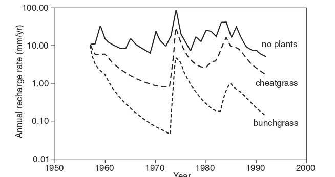
FIGURE3.14 Simulated recharge rates for Ephrata sandy loam and three different vegetation covers, Hanford Site, WA. (From Fayer and Walters, 1995.)
Variations of precipitation and air temperature are also very important for recharge. In some years it may never rain (or snow) enough to cause any recharge in semiarid climates with high PET. Even that portion of rainfall that infiltrates into the shallow subsurface may be evapotranspired back to the atmosphere before it percolates deeper than the critical depth of ET. Higher air temperatures cause more ET from the shallow subsurface and a higher soil moisture deficit (drier soil).
The impact of vegetative cover on recharge also depends on climatic variations. Dur-ing drier and warmer years, plants will uptake a higher percentage of the infiltrated water than during average years, and this will also vary for different plant species. What all this means is that the relationship between precipitation and actual groundwater recharge is not linear; simply adopting values of certain quantitative parameters measured during 1 or 2 years, as representative of the long-term groundwater recharge would be erroneous. Figure 3.14 illustrates some of the above points. Recharge rates for a 30-year period were simulated for different vegetation covers based on extensive site-specific, multiyear field analyses of various soil properties, vegetation root density, root water uptake, and infil-tration rates (Fayer and Walters, 1995). The starting point for all three simulations was the same soil water content in 1957. The model-simulated recharge rates show two orders of magnitude difference in recharge for soil with bunchgrass, compared to one order of magnitude difference for nonvegetated soil. At the same time, there is much less overall variation in recharge for the vegetated than for the nonvegetated soil.
The above short discussion on the role of climate variability shows that in any given case (e.g., vegetated or nonvegetated soil, type of vegetative cover, and type of soil), it is very important to account for the type and temporal variability of precipitation, as well as the variability of air temperature, if one were to base groundwater management decisions on any time-dependent basis.
3.5.2
Geology and Topography
FIGURE3.15 Subvertical layers of limestone near land surface and thin residuum enhance aquifer recharge. Zlatar karst massif in western Serbia.
bedding greatly increase infiltration (Fig. 3.15), while layers of unfractured bedrock slop-ing at the same angle as the land surface may almost completely eliminate it.
Mature karst areas, where rock porosity is greatly increased by dissolution, generally have the highest infiltration capacity of all geologic media. For example, actual aquifer recharge rates of over 80 percent of total precipitation, even for high-intensity rainfall events of more than 250 mm/day, have been routinely recorded in classic karst areas of Montenegro. These rates were determined by measuring flow of large temporary karst springs, which would become active within only a few hours after the start of rainfall. Several temporary springs in the area have recorded maximum discharge rate of over 300 m3/s and are among the largest such springs in the world (Fig. 3.16).
FIGURE3.16 Karst spring Sopot on the Adriatic coast of Montenegro discharging over 200 m3/s within 24 h of a summer storm. Before the storm, the spring was completely dry. (Photograph courtesy of Igor Jemcov.)
contribute to increased infiltration as discussed earlier; the same is true for northern slopes.
3.5.3
Land Cover and Land Use
Because of the time lag between surface water processes, including infiltration, and the actual groundwater recharge arriving at the water table, it is very important to take into consideration historic land use and land cover changes when estimating representative recharge rates. It is equally important to consider future land use changes when making predictions or when modeling groundwater availability.
formation of fine-sediment deposits along stream channels, which reduces hydraulic con-nectivity and exchange between surface water and groundwater in river flood plains. Clear-cutting of forests also alters the hydrologic cycle and results in increased erosion and sediment loading to surface streams. Conversion of low-lying forests into agricul-tural land may increase groundwater recharge, especially if it is followed by irrigation. However, it is important to remember that often this additional recharge is irrigation return, and the origin of water may be the underlying aquifer in question. In such case, irrigation return would be a small fraction of the groundwater originally pumped. In con-trast, cutting of forests in areas with steeper slopes will generally decrease groundwater recharge because of the increased runoff, except in cases of very permeable bedrock, such as karstified limestone at or near land surface.
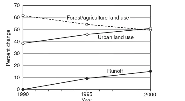
The evolution of land use in the United States follows a typical pattern outlined by Taylor and Acevedo (2006). During the eighteenth and nineteenth centuries, natural for-est or grassland habitat was extensively converted to agricultural use. The industrial revolution of the late nineteenth and early twentieth centuries spurred urban develop-ment and massive migration to city centers. Agricultural land was extensively reforested during this time period, either naturally or artificially. Following World War II, devel-opment patterns took on a more “modern” approach, as people moved out of cities into peripheral suburban communities. During this phase, which is still taking place, both agricultural and forested lands are converted to residential, commercial, and industrial areas, as jobs tend to rapidly follow Americans to the suburbs. Figure 3.17 shows land use changes in central and southern Maryland, an area experiencing dramatic sprawl due to expansion from Washington, DC, and Baltimore metropolitan areas.
Using the SCS CN method, one can approximate changes in runoff over time in the study area. Data from the Cub Run Watershed in Northern Virginia illustrate how land use changes impact runoff. A weighted approach to the SCS method was applied to derive one CN for the entire watershed. The basic procedure is multiplying the percent of the watershed comprising a certain land use by the CN corresponding to that land use and then calculating the summation of all such products. The study in the Cub Run Watershed begins in 1990, well after the transition from agricultural land to forest land.
Agriculture
Forest
Urban
1850 1900 1950 1972 1984 1992
Year
Runoff Urban land use Forest/agriculture land use
Per
cent
chang
e
Year 70
60
50
40
0 10 20 30
1990 1995 2000
FIGURE3.18 Runoff changes in Cub Run watershed, northern Virginia.
Between 1990 and 2000, land was rapidly converted to urban use, consisting of higher density residential and commercial developments (Dougherty et al., 2004). The effects of these changes result in an approximate 15 percent increase in runoff from the watershed, as shown in Fig. 3.18. The increase in runoff means less groundwater recharge in the watershed and more erosion of streambanks and impairment of water quality.
A similar analysis for watersheds in California reveals the same trend, namely, that rapid urbanization leads to exponential growth in runoff (Warrick and Orzech, 2006). Figure 3.19 shows the annual average discharge normalized by precipitation for four rivers in Southern California from 1920 to 2000. The construction of dams for flood control purposes on the Santa Ana and Los Angeles rivers only temporarily delayed dramatic increases in river discharge. A significant portion of this runoff was once groundwater recharge, placing further strain on over-allocated aquifers in the region. Figure 3.20 shows how the cumulative sediment discharge of the Santa Ana River also increased between 1970 and 2000 as a consequence of urbanization and the increase in runoff. This and many other similar studies show that city planners and water managers must promote infiltration in urban and suburban environments, both to reduce runoff and erosion and to sustain groundwater resources.
As previously discussed, urban development often causes decreases in infiltration rates and increases in surface runoff because of the increasing area of various imper-vious surfaces (rooftops, asphalt, and concrete). However, Table 3.2 illustrates that the infiltration rate varies significantly within an urban area based on actual land use. This is particularly important when evaluating fate and transport of contaminant plumes, including development of groundwater models for such diverse areas. For example, a contaminant plume may originate at an industrial facility, with high percentage of im-pervious surfaces resulting in hardly any actual infiltration, and then migrate toward a residential area where infiltration rates may be rather high because of the open space (yards) and irrigation (watering of lawns).
Santa Ana River Los Angeles River
1920 1940 1960 1980 2000
1920 1940 1960 1980 2000
Prado Dam
1920 1940 1960 1980 2000 1920 1940 1960 1980 2000
FIGURE3.19 The time history of the relationship between river discharge and precipitation for southern California rivers showing increases in discharge with respect to precipitation. All records have been normalized by the annual precipitation measured at Santa Ana, CA. Solid lines show 10-year means; shadings are 1 standard deviation about the means. (From Warrick and Orzech, 2006.)
changes in water-rock reactions in soils and aquifers caused by increased concentrations of dissolved oxidants, protons, and major ions. Agricultural activities have directly or indirectly affected the concentrations of a large number of inorganic chemicals in ground-water, such as NO−
3, N2, Cl, SO42−, H+, P, C, K, Mg, Ca, Sr, Ba, Ra, and As, as well as a
wide variety of pesticides and other organic compounds (B ¨ohlke, 2002).
3.6 Methods for Estimating Groundwater Recharge
Direct quantitative measurements of groundwater recharge flux, actually arriving at the water table and determined as volume per time (e.g., ft3/day or m3/day) are
0
FIGURE3.20 Cumulative sediment loads for the Santa Ana River and Santa Clara during 1965 to 2000. Dashed line represents a constant relationship in sediment loads; gray shade is the accumulated standard error of the cumulative loads. Inserts represent sediment load pattern for the Santa Ana River. (From Warrick and Orzech, 2006.)
rates and other hydrogeological factors” (Foster, 1988). Similarly, “Groundwater recharge estimation must be treated as an iterative process that allows progressive collection of aquifer-response data and resource evaluation. In addition, more than one technique needs to be used to verify results” (Sophocleous, 2004).
Indirect estimates of groundwater recharge have numerous limitations, particularly in arid environments. First and foremost, calculations are highly sensitive to changes in physical and empirical matric head-moisture curve fit parameters. This problem is
Area Precipitation Recharge
Land Use and Land Cover (mi2) (in/yr) (in/yr) Recharge %
Undeveloped and nonbuilt-up 641 44.2 24.1 54.5
Residential 13 43.3 12.7 29.3
Built-up 35 45.0 13.3 29.6
Urban 99 43.7 8.1 18.5
All categories 788 44.2 21.4 48.4
Modified from Lee and Risley (2002).
exacerbated at low moisture contents in arid environments, where order of magnitude changes in flux result from small variations in physical measurements. These difficulties are especially problematic for the Darcian and numerical modeling methods, which rely on limited point measurements of pressure head, unsaturated hydraulic conductivity, and moisture content. The water table fluctuation method experiences similar problems in semiarid settings due to the significant time lag between infiltration at the ground surface and a corresponding rise in the water table (Sophocleous, 2004).
Another major problem with indirect physical methods is their reliance on idealized, theoretical equations, which do not accurately depict flow mechanisms in the vadose zone. It has been known for decades that infiltration occurs in the form of an uneven front even in seemingly homogeneous soils. This can be explained by a number of differ-ent mechanisms that can form such preferdiffer-ential flow paths (“channeling”): wormholes, fractures, dendritic networks of enhanced moisture, and contact points of differing soil media (Nimmo, 2007). Water velocity through these “macropores” is often an order of magnitude greater than movement through the soil matrix. The macropores issue may further complicate measurement in semiarid and arid environments, where normally dry fractures may only become activated after threshold rainfall events. In humid envi-ronments, higher moisture contents persist in surface soils and there is less sensitivity with regard to pressure head and unsaturated hydraulic conductivity. The water table fluctuation method is also more useful, as immediate changes in water table elevation are visible after recharge events (Sophocleous, 2004). To summarize, indirect physical methods are better suited in humid climates where water managers can have a better handle on the water balance. Heterogeneity and hydraulic sensitivity dominate semiarid and arid environments, where the influence of preferential flow through macropores fur-ther compromises accuracy of recharge estimates. When measured physical parameters fall in the dry range, recharge flux calculations are often in error by at least an order of magnitude (Sophocleous, 2004). Recommendations on choosing appropriate techniques for quantifying groundwater recharge are given by Scanlon et al. (2002).
3.6.1
Lysimeters
The most common procedure for direct physical measurement of recharge flux (net in-filtration) involves the construction of lysimeters. Lysimeters are vessels filled with soil that are placed below land surface and collect the percolating water. The construction and design of lysimeters vary significantly depending on their purpose. Figures 3.21 and 3.22 show one of the most elaborate and expensive lysimeter facilities today, designed to directly measure various quantitative and qualitative parameters of water migrating through the vadose zone. Lysimeter stations may be equipped with a variety of auto-mated instruments including tensiometers, which measure matric potential at different depths and instruments that measure actual flux (flow rate) of infiltrating water at dif-ferent depths. Some stations may also include piezometers for recording water table fluctuations. Water quality parameters may also be measured and recorded automati-cally.
FIGURE3.21 Array of lysimeters operated by Helmholtz Center Munich—German Research Center for Environmental Health (GmbH). (Photograph courtesy of Dr. Sascha Reth.)
Lysimeters may have varying degrees of surface vegetation and may contain dis-turbed or undisdis-turbed soil. The clear advantage of lysimeters is that they enable direct measurement of the quantity of water descending past the root zone over a time period of interest. Net infiltration flux is easily calculated from these measurements, eliminating much uncertainty in surficial processes such as ET and runoff. Lysimeters also capture infiltration moving rapidly through preferential flow pathways like macropores and fractures. The main disadvantages of lysimeters are their expensive construction costs and difficult maintenance requirements. These costs generally limit the total depth of lysimeters to about 10 ft, which inhibits direct correlation of net infiltration with actual groundwater recharge, since low-permeability clay layers may lie below the bottom of the lysimeter (Sophocleous, 2004). Additionally, lysimeters constructed with disturbed soils may have higher moisture contents, possibly skewing measurement results and overestimating recharge.
A major difficulty when extrapolating lysimeter data to a wider aquifer recharge area is the inevitably high variability in soil and vegetative characteristics. A recent study by the USGS (Risser et al., 2005a) illustrates this problem. Data collected from seven lysime-ters installed on a 100 ft2plot show that the coefficient of variation between monthly
recharge rates at individual lysimeters is greater than 20 percent for 6 months, with the June, July, and August values of about 50, 100, and 60 percent, respectively. Coordinat-ing direct measurements with a water balance or water table fluctuation approximation on a larger scale may help resolve some of the scale problems associated with point measurements using lysimeters.
3.6.2
Soil Moisture Measurements
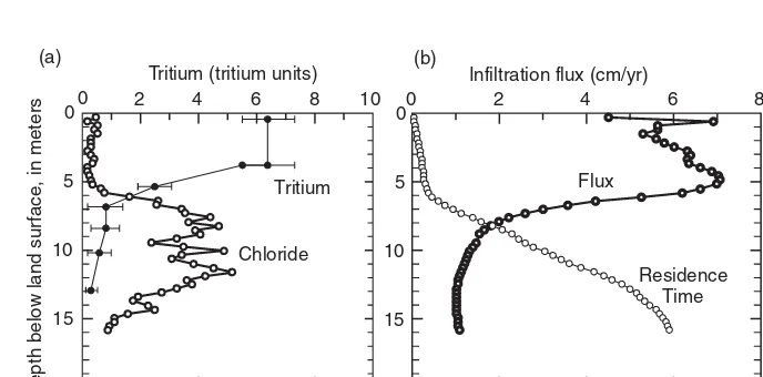
Small negative pressure heads (less than about 100 kPa) in the unsaturated zone can be measured with tensiometers, which couple the measuring fluid in a manometer, vac-uum gauge, or pressure transducer to water in the surrounding partially saturated soil through a porous membrane. The pressure status of water held under large negative pressures (greater than 100 kPa) may be measured using thermocouple psychrometers, which measure the relative humidity of the gas phase within the medium and with heat dissipation probes or HDPs (Lappala et al., 1987; McMahon et al., 2003). The measuring instrumentation may be permanently installed in wells screened at different depths to measure soil moisture profile in the vadose zone, or measurements may be performed on a temporary basis using direct push methods, such as cone penetrometers equipped with tension rings. In shallow applications, soil moisture probes can be installed in trenches. By simultaneously measuring the matric potential and the moisture content at same vertical locations during different hydrologic conditions (e.g., prior, during, and after periods of major recharge), it is possible to plot several moisture characteristic curves, which then enables accurate determination of the unsaturated hydraulic conductivity and calculations of flow rates and velocities in the unsaturated zone. This method also helps to distinguish between the relative proportions of net water loss to evaporation (upward water movement) and drainage (downward water movement) by establishing a plane of zero potential gradient, called “zero flux” plane (Fig. 3.23).
3.6.3
Water Table Fluctuations
Water
Soil moisture content Soil water potential
D
= Water lost to evaporation = Water lost to drainage
Determined from soil moisture
FIGURE3.23 Illustration of the measurement of evaporation using soil moisture depletion supplemented with the determination of an average “zero flux” plane to discriminate between (upward) evaporation and (downward) drainage. (From Shuttleworth, 1993; copyright McGraw-Hill.)
to the product of water table rise and specific yield (Fig. 3.24):
R=Syh (3.22)
where R=recharge (L)
Sy=specific yield (dimensionless)
h=water table rise (L).
Because of its simplicity and general availability of water-level measurements in most groundwater projects, the water table fluctuation method may be the most widely used method for estimating recharge rates in humid regions.The main uncertainty in applying this approach is the value of specific yield, which, in many cases, would have to be assumed.
An important factor to consider when applying water table fluctuation method is the frequency of water-level measurement. Delin and Falteisek (2007) point out that measurements made less frequently than about once per week may result in as much as a 48-percent underestimation of recharge based on an hourly measurement frequency.
Zaidi et al. (2007) used the double water table fluctuation method and an extensive network of observation wells to calculate water budget for a semiarid crystalline rock aquifer in India. The monsoonal character of rainfall in the area allows division of the hydrologic year into two distinct dry and wet seasons and application of the following water budget equation twice a year:
R+RF +Qin=E+PG+Qout+Syh (3.23)
where two parameters, natural recharge,R, and specific yield,Sy, are unknown. Water
table fluctuations,h, are measured, and other components of the water budget are independently estimated:RFis the irrigation return flow, Qinand Qoutare horizontal
inflows and outflows in the basin, respectively,Eis evaporation, andPGis groundwater extraction by pumping. The method is called the “double water table fluctuation” be-cause the equation is applied two times (for wet and dry season) so that both unknowns (recharge and specific yield) can be solved. This eliminates inaccuracies associated with estimating specific yield at large field scales.
3.6.4
Environmental Tracers
of magnitude shows that preferential flow in some cases may be a dominant recharge mechanism and illustrates the major need for more research in this area (Sophocleous, 2004).
Environmental tracers commonly used to estimate the age of young groundwater (less than 50 to 70 years old) are the chlorofluorocarbons (CFCs) and the ratio of tritium and helium-3 (3H/3He). Because of various uncertainties and assumptions that are
as-sociated with sampling, analysis, and interpretation of the environmental tracer data, groundwater ages estimated using CFC and3H-3He methods are regarded as apparent
ages and must be carefully reviewed to ensure that they are geochemically consistent and hydrologically realistic (Rowe et al., 1999). Isotopes typically used for the determina-tion of older groundwater ages are carbon-14, oxygen-18 and deuterium, and chlorine-36, with many other isotopes are increasingly studied for their applicability (Geyh, 2000).
Although reference is often made to dating of groundwater, the age actually applies to the date of introduction of the tracer substance and not the water. Unless one recognizes and accounts for all the physical and chemical processes that affect the concentrations of an environmental tracer in the aquifer, the tracer-based age is not necessarily equal to the transit time of the water (Plummer and Busenberg, 2007). The concentrations of all dissolved substances are affected, to some extent, by transport processes. For some tracers, the concentrations can also be affected by chemical processes, such as degradation and sorption during transit. For this reason, the term “age” is usually qualified with the word “model” or “apparent,” i.e., “model age” or “apparent age.” The emphasis on model or apparent ages is needed because simplifying assumptions regarding the transport processes are often made and chemical processes that may affect tracer concentrations are usually not accounted for (Plummer and Busenberg, 2007).
Detailed international field research on the applicability of isotopic and geochemical methods in the vadose (unsaturated) zone for groundwater recharge estimation was coordinated by the International Atomic Energy Agency (IAEA) during 1995 to 1999, with results obtained from 44 sites mainly in arid climates (IAEA, 2001). Information on the physiography, lithology, rainfall, vadose zone moisture content, and chemical and isotopic characteristics was collected at each profiling site and used to estimate contemporary recharge rates (see Table 3.3 for examples).
The best source for numerous studies on the application of various environmental iso-topes in surface water and groundwater studies are the proceedings of the international conferences organized by the IAEA as well as the related monographs published by the agency, many of which are available for free download at its Web site (www.iaea.org).
Chloride
Mass balance of a natural environmental tracer in the soil pore water may be used to measure infiltration where the sole source of the tracer is atmospheric precipitation and where runoff is known or negligible. The relationship for a steady-state mass balance is (Bedinger, 1987)
Rq=(P−Rs)
Cp
Cz
(3.24)
where Rq(infiltration) is a function ofP (precipitation), Rs (surface runoff),Cp(tracer