Published online 11 March 2008 in Wiley InterScience (www.interscience.wiley.com) DOI: 10.1002/hyp.6989
Reconciling theory with observations: elements of a
diagnostic approach to model evaluation
Hoshin V. Gupta,
1* Thorsten Wagener
2and Yuqiong Liu
1 1SAHRA, Department of Hydrology & Water Resources, The University of Arizona, Tucson AZ 85721 2Department of Civil and Environmental Engineering, Pennsylvania State University, University Park, PA 16802Abstract:
This paper discusses the need for a well-considered approach to reconciling environmental theory with observations that has clear and compelling diagnostic power. This need is well recognized by the scientific community in the context of the ‘Predictions in Ungaged Basins’ initiative and the National Science Foundation sponsored ‘Environmental Observatories’ initiative, among others. It is suggested that many current strategies for confronting environmental process models with observational data are inadequate in the face of the highly complex and high order models becoming central to modern environmental science, and steps are proposed towards the development of a robust and powerful ‘Theory of Evaluation’. This paper presents the concept of a diagnostic evaluation approach rooted in information theory and employing the notion of signature indices that measure theoretically relevant system process behaviours. The signature-based approach addresses the issue of degree of system complexity resolvable by a model. Further, it can be placed in the context of Bayesian inference to facilitate uncertainty analysis, and can be readily applied to the problem of process evaluation leading to improved predictions in ungaged basins. Copyright2008 John Wiley & Sons, Ltd.
KEY WORDS model identification; information; evaluation; diagnosis; signatures; uncertainty
Received 26 June 2007; Accepted 15 December 2007
INTRODUCTION
The trend in environmental modeling is towards ever more complex and physically realistic representations of the dynamic behaviour of the earth system, driven by the need for better management of increasingly scarce resources, and by the recent rapid pace of improved eco-geo-hydro-meteorological understanding. Strong tech-nological drivers are also at work, with increasingly more powerful computers, distributed flux and land sur-face data (including remote sensing), improved cyber-infrastructure (including the WWW), and sophisticated modeling toolboxes.
As we build more realistic and detailed models of environmental processes, we must also develop methods powerful enough to evaluate (test) and correct them (Spear and Hornberger, 1980; Guptaet al., 1998; Beven, 2001; Wageneret al., 2003b; Wagener and Gupta 2005, among others). In particular, such methods must be ‘diagnostic’, meaning they must help illuminate to what degree a realistic representation of the real world has (or has not) been achieved and (more importantly) how the model should be improved. Because more complex process representations lead (unavoidably) to greater interaction among model components, the limitations of ad hoc evaluation approaches will become increasingly
* Correspondence to: Hoshin V. Gupta, SAHRA, Department of Hydrol-ogy & Water Resources, The University of Arizona, Tucson AZ 85721. E-mail: [email protected]
apparent and the demand for more power in identification methods will grow (Wagener and Gupta, 2005).
There is, therefore, a strong need for sophisticated approaches to model evaluation, and this need is becom-ing well recognized in the scientific community. For example, the Predictions in Ungaged Basins (PUB) initia-tive seeks to reduce predicinitia-tive uncertainty through inter-active learning leading to new and/or improved hydro-logical models (Sivapalan et al., 2003a); Theme 3 of the PUB initiative is titled ‘Uncertainty Analysis and Model Diagnostics’ (Wagener et al., 2006). A broader community effort involves the move towards Environ-mental Observatories (EOs) in the USA and elsewhere. As stated during a recent National Science Foundation (NSF) sponsored meeting to discuss Grand Challenges of the Future for Environmental Modeling: ‘Models are complex assemblies of multiple, constituent hypotheses . . .that must be tested. . .against the new streams of field data. Working out novel ways of conducting these tests, will be a major scientific challenge associated with the Environmental Observatories’ (Beck, Presentation at NSF EO Workshop on Modeling, Tucson, AZ, April 2007). This is further expressed as Challenge # 7 in the white paper resulting from the workshop:
environmental knowledge —this given the expected massive expansion in the scope and volume of field observations generated by the Environmen-tal Observatories, coupled and integrated with the prospect of equally massive expansion in data pro-cessing and scientific visualization enabled by the future environmental cyber-infrastructure? (Beck et al., 2007).
In other words, how do we take large models and large volumes of data, juxtapose (compare and contrast) them, and make sense of this juxtaposition?
It is the thesis of this paper that a robust and powerful ‘Theory of Evaluation’ is needed, i.e. a well-considered approach to reconciling environmental theory with obser-vations, that has clear and compelling diagnostic power. The current strategies for confronting models with data are largely rooted either in ad-hoc manual-expert model evaluation or in statistical regression theory. It is sug-gested that these strategies, while capable in the case of relatively simple models, will prove wholly inadequate in the face of the highly complex models central to modern environmental science.
The aim of this paper is to propose some elements of a path towards a diagnostic approach to model evaluation. The following two sections present a conceptual descrip-tion of model development and the consequent basis for model evaluation. The diagnostic problem is discussed in the fourth section, followed by two sections address-ing the nature of information and the related concept of signature behaviours. The seventh section proposes a framework for a diagnostic approach to model evaluation based on signature index matching. The final two sections discuss how the signature-based approach can be framed within the context of Bayesian uncertainty analysis, and
how it applies to the problem of prediction in ungauged basins.
CONCEPTUAL DESCRIPTION OF THE MODEL BUILDING PROCESS
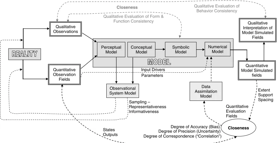
A model is a simplified representation of a system, whose two-fold purpose is to enable reasoning within an ide-alized framework, and to enable testable predictions of what might happen under new circumstances. Done prop-erly, the representation is based on explicit simplifying assumptions that allow acceptably accurate simulations of the real system. A compact overview of the model build-ing and evaluation process is presented in Figure 1. We begin by interacting with reality through observation and experiment (through our senses and measurement device extensions of our senses). From qualitative and quan-titative observations of the environmental system, we gain a progressive mental understanding of what seems important and how things work. This coalesces into a subjective ‘perceptual model’, unique to each person and conditioned on (influenced by) previous experience and education.
As we organize and formalize this perceptual (mental) understanding through contemplation and discussion, one or more ‘conceptual models’ emerge, represented usu-ally in the form of verbal and pictorial descriptions that enable us to specify, summarize and discuss our under-standing with other people. A complete conceptual model will include a clear specification of the following system elements; system boundaries, relevant inputs, state vari-ables and outputs, physical and/or behavioural laws to be obeyed (e.g. continuity of mass, momentum, etc.), facts to be properly incorporated (e.g. spatio-temporal distribu-tion of ‘static’ material properties such as soils), uncer-tainties to be considered, and the simplifying assumptions
Qualitative Observations
Quantitative Observation
Fields
Perceptual Model
Conceptual Model
Symbolic Model
Numerical Model
Quantitative Model Simulated
fields Qualitative Interpretation of Model Simulated
Fields
Observational System Model
Data Assimilation
Model
Closeness
Closeness
Qualitative Evaluation of Form & Function Consistency
Qualitative Evaluation of Behavior Consistency
Extent Support Spacing
Quantitative Evaluation Fields
Degree of Accuracy (Bias) Degree of Precision (Uncertainty) Degree of Correspondence (“Correlation”) States
Outputs
Sampling – Representativeness Informativeness
Input Drivers Parameters
to be made. The relationships among these elements need not be rigorously specified, but should be conceptually explained through drawings, maps, tables, papers, reports, oral presentations, etc. Therefore, the conceptual model summarizes our abstract state of knowledge (degree of belief) about the structure and workings of the system. Further, it defines the level at which communication actu-ally occurs between scientific colleagues or between sci-entists and policy/decision makers (Gupta et al., 2007; Liuet al., 2007). Alternative conceptual models represent competing hypotheses about the structure and functioning of the observed system, conditioned on the perceptually acquired qualitative and quantitative observations and on the prior facts/knowledge/ideas. Taken together, the per-ceptual and conper-ceptual models of the system along with the conditioning prior knowledge form the rudimentary levels of our ‘theory’ about the system.
The need to better understand the system and to bet-ter discriminate between competing hypotheses leads to the formulation of an ‘observational system model’ (not to be confused with the observation model of data assimilation) to guide effective and efficient acquisi-tion of further data. The observaacquisi-tion model should, of course, be derived from the theory and be designed to maximally reduce the uncertainty in our knowl-edge (conditioned unavoidably on the correctness of the theory). Further, it should also be designed to diag-nostically detect flaws in the theory (a more difficult challenge). Observational model design should accom-modate observations on boundary conditions, conven-tional and extreme modes of system behaviour, the issue of poorly observable system states, clarification of assumptions, and so on. Design issues will include (a) sufficiency of sampling, (b) representativeness of observations, (c) informativeness and quality of data, and (d) measurement extent, support and spacing (see discus-sion in Grayson and Bl¨oschl, 2000). Clearly, acquisition of knowledge via the observational system model is com-plementary to the formation of hypotheses via the theory. The proper design of an evaluation procedure becomes critically important, therefore, as the constituent hypothe-ses and sources of information become increasingly com-plex. In the ideal, a comprehensive evaluation procedure would help to evaluate the entire ‘theory’, instead of only a comparison of one or more model outputs against the corresponding observations, as is typically the case.
The next steps in model development include the for-mulation of ‘symbolic’ and ‘numerical’ models. A sym-bolic model formalizes the understanding represented by a conceptual model using a mathematical system of logic that can be manipulated to enable rigorous reasoning and to facilitate the formulation of testable predictions (the two purposes of a model mentioned earlier). It is com-mon to use the related systems of algebra and calculus for this purpose, although other logical systems are pos-sible. Finally, because mathematical intractability often precludes explicit derivations of the dynamic evolution of system trajectories, it is common to build a numeri-cal model approximation using a computer. We will not
debate the relative merits of the explicit and implicit solution approaches here. However, to acquire a proper understanding of complex environmental systems via the numerical modeling approach we must typically examine a very large number of representative simulation runs that span the extent of the behavioural model space. Again, this speaks to the need for proper design of a model evaluation procedure.
EVALUATION OF NUMERICAL MODELS
Hereafter, unless otherwise mentioned, we use the term ‘model’ to refer to a computer-based numerical model that provides dynamic simulations of system input-state-output (I-S-O) behaviour, and understand that its validity is conditioned on the correctness of the underlying per-ceptual, conceptual and symbolic models of the system. Our confidence in its use for reasoning and the formu-lation of testable predictions will depend on how ‘close’ the model is to reality. In operational forecasting (e.g. flood forecasting, numerical weather prediction) we are typically more concerned with the accuracy (unbiased-ness) and precision (minimality of uncertainty) of the model simulations than in the correctness of the model structural form. There, it is common to use data assim-ilation to merge model predictions with spatio-temporal flux and state observations, a process rooted in Bayesian mathematics and incorporating an appropriate model of the observation process (Liu and Gupta, 2007). The liter-ature includes applications of the Kalman Filter (Kalman, 1960), Ensemble Kalman Filter (Evensen, 1994), and various Bayesian approaches such as particle filtering (Gordonet al., 1993; Moradkhaniet al., 2005), Bayesian recursive estimation (Thiemann et al., 2001), and the data-based mechanistic (DBM) approach to stochastic modeling (Young, 2002, 2003; Romanowiczet al., 2006; Young and Garnier, 2006). These approaches depend on a relative assessment of the ‘correctness’ of the model simulation and its associated observation to make an interpolative (typically linear) correction to the modeled estimate of the system state; the problem is discussed in detail in Liu and Gupta (2007). Here we focus attention on the more important problem of model evaluation; i.e. how to link what we ‘see’ in the data to what is ‘right’ and ‘wrong’ with the model(s). This knowledge can then be used to reject underlying hypotheses, develop improved models and advance theory (Wagener, 2003).
mentioned earlier, sufficiency of sampling, representa-tiveness, informativeness and data quality must also be considered. Equally important, we must consider the degree of accuracy (bias), degree of precision (uncer-tainty) and degree of correspondence and/or commen-surability (‘sameness’ of the quantities in question) in the comparative evaluation of both fields. Measurable similarities will lend support towards the constituent model/hypothesis, while measurable differences will lend support against. The question is just how the comparison should be done and how the results are to be interpreted. The typical approach to quantitative evaluation is to construct a regression measure, most commonly some form of mean (weighted) squared error between the observed and model simulated fields, that describes in some average mathematical sense the ‘size’ of the dif-ferences between the two fields. In the more sophisti-cated Likelihood approach, a measure is constructed that describes instead how ‘likely’ it is that the observed fields ‘could have been’ generated (again in some average sense) by the constituent Model/Hypothesis. However, it is increasingly recognized that such measures of aver-age model/data similarity inherently lack the ‘power’ to provide a meaningful comparative evaluation (more on this later) (Gupta et al. 1998, 2005; Wagener and Gupta, 2005). Further, it has always been the case that less formal consistency checks (qualitative evaluations of consistency in model behaviour) have been central to any meaningful model evaluation; historically this has taken a wide variety of forms, ranging from visual eval-uations of spatio-temporal patterns (e.g. hydrographs), to scatter-plots comparing observed and simulated variables, to tests of behavioural compliance (e.g. the emergence of expected behaviour such as algae bloom) (Spear and Hornberger, 1980). More recently, it has become com-mon to also incorporate qualitative, but formal, measures of consistency between model behaviour and the observa-tions, through use of mathematical strategies such as gen-eralized likelihood approaches (Beven, 2006) and fuzzy set theory (Seibert and McDonnell, 2002).
An approach that combines quantitative and qual-itative approaches to evaluating the consistency of model behaviour is to test for parameter variation in time (Wagener, 2003). In their multi-objective approach, Gupta et al. (1998) showed that hydrological models could fail to represent different response modes of a sys-tem with a sys-temporally invariant parameter set; this indi-cates that some aspect of the underlying model hypothesis is invalid and should be improved. It has been sug-gested that the time variation of parameters can be used to provide guidance for potential model improvement, and various techniques have been proposed to formalize this style of analysis (Beck, 1985; Wageneret al., 2003a; Young and Garnier, 2006; Lin and Beck, 2007).
Finally it should not be forgotten that a strong, albeit subjective, test has always been the ‘qualitative evalu-ation of consistency in model form and function’. By ‘form’ we mean the structure of the model/system, and by ‘function’ we mean its behavioural capability (Wagener
et al., 2007). Critical support for a model (or theory) is generally stronger if there is a clear isomorphic relation-ship between the model and the system at the percep-tual/conceptual/symbolic levels; e.g. a partial differential equation based I-S-O representation of watershed dynam-ics is generally considered superior to a conceptual-tank based I-S-O representation, which in turn is considered superior to an artificial neural network I-O based rep-resentation. This is particularly true when the model is intended to support both scientific reasoning and testable predictions aimed at improving underlying understand-ing about the system. However, when testable prediction is of prime concern, as in operational forecasting, the order of preference is somewhat less clear (Wagener and McIntyre, 2005).
To summarize, there are three kinds of closeness that must be incorporated into a formal theory of evaluation:
a) quantitative evaluation of behaviour; b) qualitative evaluation of behaviour, and c) qualitative evaluation of form and function.
THE DIAGNOSTIC PROBLEM
As commonly employed, the evaluation framework described above is weak in a diagnostic sense. Since the main reason to confront models/hypotheses/theories with observational data is not so much to ‘validate’ what we believe to be true, (clearly difficult in any case, see Oreskes et al., 1994; Popper, 2000; and others), but to detect and ‘diagnose’ what remains wrong with our con-ceptions. Much time and energy however is still spent on attempts at model ‘validation’, in an arguably misguided attempt to defend the existing model, often without refer-ence to any alternative model, hypothesis or theory. The vast majority of model ‘validations’ are justified by show-ing graphical plots of similarity between observed and model simulated hydrographs, accompanied by statistics such as the ‘Nash efficiency’ or ‘correlation coefficient’. It seems poorly recognized that the Nash efficiency sum-marizes model performance relative to an extremely weak benchmark (the observed mean output) and has no basis in underlying hydrologic theory (Seibert, 2001; Schaefli and Gupta, 2007). Given that much of the variability in the observed streamflow hydrograph is the direct conse-quence of variability in the rainfall (or snowmelt), hydro-graph comparisons often reveal little about how much of the underlying I-S-O watershed transformation pro-cess has actually been captured by the model (yes, the observed and simulated hydrographs go up and down at the same time, but so what?).
increasingly complex models. This seems a lazy approach to science, particularly if we have not properly tested the limits of agreement (or lack thereof) between our models and the data. We expand on the notion of information in the next section. Here, we define the ‘diagnostic prob-lem’ as:
The Diagnostic Problem (Definition):.Given a com-putational model of a system, together with a sim-ulation of the systems behaviour which conflicts with the way the system is observed (or sup-posed) to behave, the diagnostic problem is to deter-mine those components of the model, which when assumed to be functioning properly, will explain the discrepancy between the computed and observed system behaviour (adapted from Reiter, 1987).
In other words, the purpose of evaluation must be ‘diagnostic’ in focus. Its goals must be: (a) to deter-mine what information is contained in the data and in the model, and (b) to determine whether, how, and to what degree the model/hypothesis is capable of being reconciled with the observations. At its strongest, a diag-nostic evaluation will point clearly towards the aspects of the model that need improvement, and give guidance towards the manner of improvement. As a corollary, it must also guide the acquisition of new observations capa-ble of evaluating (and possibly invalidating) the current best hypothesis about the system.
The problem of diagnosis is, of course, general to all spheres of decision-making, not just science, pre-cisely because all decision-making is dependent on some underlying model of a system. In mechanics, electrical engineering, the petroleum industry and numerous other fields, we use observations of abnormal system behaviour to diagnose faulty components (Trave-Massuyes and Milne, 1997; Friedrichet al., 1999; Peischl and Wotawa, 2003). In medicine, a doctor is trained to hypothesize possible medical conditions of the body from a variety of ‘symptoms’, obtained by both subjective questioning of the patient and by means of objective tests (Swartz, 2001). There are (at least) two kinds of diagnostic proce-dures, namely correlative and causal. A correlative diag-nostic is one established through direct observation of a strong (linear or non-linear) correlative relationship; e.g. abnormalities in the patterns of stock prices can be cor-related with indices of the psychological state of a pop-ulation (Saunders Jr, 1993). No strong theory explaining the relationship between the various co-related variables is necessary. A causal diagnostic, however, is one where the underlying theory can be used to actually predict the (observable) impact of system changes (or defects), and similarly to infer various possible causes of an observable system response (or deviation thereof); a trivial example is that if the model does not simulate processes associated with observed overland flow, the infiltration or saturation excess components of the model might be at fault.
The theory-based causal approach is clearly a stronger approach to diagnostic evaluation, although a correlative
approach can also lead to improved system understanding and point towards an ultimate causal basis for diagnosis. The bottom line is that, to be meaningful, procedures for evaluation and reconciliation of environmental models with observations must be rooted in and based on the underlying environmental theory.
THE ISSUE OF WHAT CONSTITUTES INFORMATION
We now discuss the foundations of a meaningful evalua-tion procedure. Leaving aside the chicken-and-egg ques-tion of which is primary, once a theory is established the scientific method proceeds in two directions, (a) to establish an experimental design for making observa-tions about the system of interest and thereby to collect data, and (b) to construct a numerical model capable of generating dynamical simulations of system behaviour. Conventional evaluation proceeds by directly confronting the model with the data, an approach that currently pro-vides little guidance to possible problems in the model hypothesis. The question is what might be a superior approach?
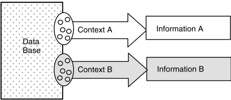
In considering this problem we quote John Gall who (reflecting on the fundamental nature of systems) sug-gests that ‘If a problem seems unsolvable . . . consider that you may have a meta-problem’, and ‘To be effective, an intervention must be introduced at the correct logical level’ (Gall, 1986). The meta-problem in this case is that, at least in the environmental sciences, ‘data’ is not the same as ‘information’. We collect data to learn something about the system, but the data consist mainly of sets of numbers. Our task is to make sense of those numbers— to detect the underlying order that enables us to make infer-ences about system structure and behaviour (form and function). So, ‘information’ is what we get when we view our data through the filter of some ‘context’ (Figure 2) provided by prior information and knowledge. A string of numbers can mean different things to different peo-ple, depending on the context each person applies— the person looking for trends in a time series has a differ-ent focus and interpretation than the person looking for periodicity— and because an infinite number of contex-tual filters can be brought to bear, the types of extractable information are similarly vast. However, our interest is the evaluation of environmental models; for this we have a very specific perspective to guide our focus, namely the underlying theoretical basis for our investigation.
In summary, information is obtained by viewing data in context (through perceptual and conceptual filtering), there may be (are usually) multiple plausible contexts, and the most relevant context is generally given by the underlying theory. Interesting questions that immediately follow include:
1) What kind of relevant information does the data contain?
Data Base
Context A
Information B Context B
Information A
Figure 2. Information is obtained by viewing and analyzing data in context
3) In what way does the extracted information support evaluation, diagnostic analysis, and eventual reconcil-iation between the theory and the observations?
Note that while extracting information by contextual filtering of the data we also perform the important func-tion of redundancy detecfunc-tion and removal. Since the data we collect are expected to reveal underlying structure (order), the dimensionRDataof the data set must be
signif-icantly larger than the dimensionRInfoof the information
it is expected to contain. So, if the dimensionRModel
rep-resents the degrees of freedom (unknowns) in the model, an optimal experimental data-gathering design will gener-ate informationRInfocapable of restricting those degrees
of freedom (i.e. RInfo¾RModel) and thereby either
sat-isfactorily constrain the residual model uncertainty, or deem the model unsatisfactory. (Remember that to unam-biguously solve a system of equations in Nunknowns, one requiresNindependent pieces of information.)
Therefore, we are also interested in relevant ‘minimal’ representations of the information contained in the data, because the amount of relevant information will enable us to know how much model complexity can actually be resolved using the data. The process of informa-tion extracinforma-tion therefore has similarities with the process of data compression; lossy compression is analogous to extracting only the most important information, while lossless compression is analogous to preserving all rel-evant information (Hankerson et al., 2003). Eventually, the numerical model we seek to construct is itself the ulti-mate attempt at lossy or lossless compression, because we expect the model to be capable of reproducing the cor-rect I-S-O behaviour under appropriate conditions. This should, we hope, help to remove lingering objections to our proposed definition of information, and to the infer-ence that ideallyRInfo¾RModel.
We propose, therefore, that a meaningful evaluation procedure must be founded in methods for extracting information from the data that are contextually relevant given the underlying theory. Just as the model is a concrete consolidation of the theory the information is a consolidation of the data, and the poorly defined problem of confronting the theory with data is abstracted to the better-defined problem of confronting the model with information. Therefore, we need to understand what kinds of information provide diagnostic power.
DIAGNOSTIC INFORMATION IN THE FORM OF SIGNATURE BEHAVIOURS
It seems important to recognize here that the ideas pre-sented above are, in part, a formal restatement of what had been common practice in environmental modeling before regression theory was applied to the problem of model identification (Guptaet al., 2005). Without access to powerful computing, model parameters would be sought that reproduced important aspects of the stream-flow hydrograph; e.g. the magnitude and timing of the peak, and the distribution of flow levels as summarized by the flow exceedance probability graph (flow duration curve) (Vogel and Fennessey, 1995). Evaluation might include a sensitivity analysis where the model response to perturbation of controlling factors would be expected to reflect similar behaviours observed in the data (Saltelli et al., 2004). Indeed, the regional sensitivity analysis approach (Spear and Hornberger, 1980) and its devel-opments (Beven and Binley, 1992) consider a model ‘behavioural’ only if it simulates certain quantitative or qualitative characteristics observed in the data. These ideas have been further codified in the argument that all model identification problems are inherently multi-criteria in nature (Guptaet al., 1998; Boyle et al., 2001; Wagener et al., 2001, 2003a, b; Vrugt et al., 2003), and that the challenge lies in (a) proper selection of measures of model performance, (b) determining the appropriate number of measures, (c) consideration of the stochastic uncertainties in the data, and (d) recognition of model error. However, although the multiple-criteria approach is now widely used, it does not (as currently applied) meet the need for diagnostic capability and power. A major goal of this paper is to explain why and thereby to suggest a suitable way forward.
From the examples mentioned, we see that the idea of characterizing ‘signature behaviours’ in the I-S-O data is not new; it is how humans naturally approach the problem of model evaluation. We detect and attend to ‘patterns’ in the data in a both conscious and unconscious search for order and meaning. The process is, of course, conditioned by oura priori knowledge — our expectations of what to look for, and our interpretations of what meanings to assign. Our environmental theory, properly applied, tells us what signature I-S-O patterns to expect (or look for) in the real world. Novel signature patterns observed in the data but not predicted to exist, or deviations in the form of observed signature patterns from those predicted, attract our attention because they suggest the existence of new information that must be properly assimilated to maintain a ‘good’ model. Attention to I-S-O signatures therefore constitutes the natural basis for diagnosis.
hydrological exploration and prediction. Rupp and Selker (2006) discuss diagnostic evaluation of the mismatch between the recession characteristics of measured and modeled flow. For other examples see Sivapalan et al. (2003b). Other early and ongoing work includes the use of attributes such as peak flow, and time to peak in the evaluation and adjustment of catchment models, and the use of ‘type curves’ to evaluate groundwater pumping or slug tests and to infer the structure of an aquifer (Moench, 1994; Illman and Neuman, 2001). Placed in this context, the body of literature is indeed large.
FRAMEWORK FOR A DIAGNOSTIC APPROACH TO MODEL EVALUATION
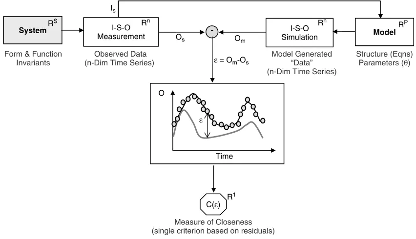
In conventional regression-based model evaluation (Figure 3) we assume that the data set DobsD fu1obs, . . . unuobs, x1obs, . . . xnxobs, y1obs, . . . ynyobsg of I-S-O
observations contains information useful for testing the hypothesis consolidated in the model; here u, x, and y represent the system inputs, state variables and outputs respectively. A corresponding set of I-S-O simulations Dsim D fu1sim, . . . unusim, x1sim, . . . xnxsim, y1sim, . . . ynysimgis generated using the model, and a residual error
sequence rDDsimDobs is constructed that measures the differences between the data and model simulation. Evaluation proceeds by selecting one or more Likelihood measuresL1⊲r⊳, . . . Lc⊲r⊳ of the “distance” between the
model and the data while accounting for measurement uncertainty. Model identification then involves optimiza-tion of the selected measures, either to drive the residual error sequence towards zero, or (more recently) to con-strain the model set to meet acceptable specifications on those measures.
In classical single-criteria regression only one likeli-hood measure is used, i.e. cD1, and the data having
dimension RData is filtered through a likelihood mea-sure having dimension R1 (commonly some form of mean squared error function) en route to an attempt to extract information about a model of dimension RModel
(Figure 4). Clearly, in projecting from the data dimension RDatato a measure dimension of ‘1’ we lose considerable amounts of information. It seems strange, and ineffi-cient, that we would attempt to extractRModel pieces of
information from the single piece of information given by the measure —the problem is clearly ill-conditioned and this has all too often been reflected in the litera-ture (Johnston and Pilgrim, 1965; Gupta and Sorooshian, 1983; Sorooshian and Gupta, 1983; Beven and Binley, 1992; Duan et al., 1993; Wagener et al., 2003b; Beven, 2006 among many others). It should be no surprise, therefore, that only low order models can be identified by this approach; note the oft made claim that only models having three to five parameters can be identi-fied from commonly available rainfall–runoff data (Jake-man and Hornberger, 1993). The very construction of the measure —as a summary (usually average) property of residual differences—dilutes and mixes the available information into an index having little remaining cor-respondence to specific behaviours of the system. So, while the classical approach works for simple (low order) models and allows for some treatment of uncertainty, it is fundamentally weak by design: (a) it fails to exploit the interesting information in the data, and (b) it fails to relate the information to characteristics of the model in a diagnostic manner.
Application of single criteria regression to environ-mental modeling violates the dictum that we should ‘make everything as simple as possible, but not sim-pler’ (attributed to A. Einstein), and as models grow more complex the problem can only get worse. Multi-criteria applications where c >1 do provide improvement; by
System I-S-O
Measurement
I-S-O Simulation RS
Model RP
-O
Time ε
Os Om
ε = Om-Os
C(ε) R1
Measure of Closeness (single criterion based on residuals) Form & Function
Invariants
Structure (Eqns) Parameters (θ) Rn
Rn Is
Observed Data (n-Dim Time Series)
Model Generated “Data” (n-Dim Time Series)
Data Dimension
Rn
Measure Dimension
R1
Parameter Dimension
RP
Figure 4. Extracting information from data using a single measure of closeness
projecting the data (dimension RData) through a filter of dimension Rc> R1 they reduce the loss of informa-tion (particularly if we properly select Rc¾RModel as discussed earlier (Gupta, 2000). However if, as is com-mon, the likelihood measures are constructed as summary statistics of the residuals, the problem of diagnostic power remains unaddressed.
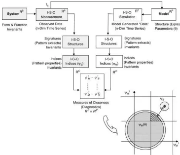
We propose that a meaningful approach to diagnostic evaluation lies through theory-based signatures extracted from the I-S-O data (Figure 5). The dataDobs should be compressed through theory-based contextual filters into I-S-O signatures (characteristic patterns) clearly related to various aspects of the theory (or characteristics of the model). Because the model is based in the theory, the relevant number and form of diagnostic signatures must arise as a consequence of the theory, and thereby
constitute testable predictions to be corroborated or falsified by the observations. The experimental design can then be properly constructed to collect data about the relevant signatures. Diagnostic evaluation consists of noting the behavioural (signature) similarities and differences between the system dataDobs and the model simulations Dsim, and correction proceeds by relating
these (symptoms of model malfunction) to relevant model components. As a trivial example, if a model is unable to reproduce observed double-peaked tracer breakthrough curves in response to an impulse input, it may indicate the absence of some constituent process. When properly rooted in theory, diagnostic evaluation can (in principle) be designed to be strongly causal. Further, the problem of evaluating highly complex and very high order models becomes clearly conditioned on the need for the (developer of the) underlying theory to propose (and demonstrate in the abstract) exactly how the proposed theory can be supported or falsified by recourse to observational processes. In fact, no model developer should be excused from this task, and no self-respecting science would settle for anything less.
FRAMING DIAGNOSTIC EVALUATION WITHIN THE CONTEXT OF BAYESIAN UNCERTAINTY
ANALYSIS
The evaluation approach described above seeks to rec-oncile models/hypotheses with data in a diagnosti-cally meaningful way. Meanwhile, Bayesian uncertainty
analysis seeks to map information from the data into information about the consistency, accuracy and precision of the data-conditioned model (Liu and Gupta, 2007). Success in either case depends on the observability and identifiability of the system when viewed through the lens of the observational model. The diagnostic evaluation approach can be framed within a Bayesian uncertainty framework in a straightforward (though not necessarily trivial) manner. As expressed concisely in 1928 by Frank Ramsey (quoted by Edwards, 1972):
In choosing a (model of a) system, we have to compromise between two principles - subject always to the proviso that the model must not contradict any effects we know, and other things being equal, we choose; a) the simplest system, and b) the system which gives the highest chance to the facts we have observed. This last is Fisher’s ‘Principle of Maximum Likelihood’, and gives the only method of verifying a system of chances.
Stated here we find the principles of consistency (to not contradict any effects we know), parsimony (to select the simplest system, all other things being equal), and maximum likelihood. It only remains to decide what the ‘facts’ are. The principle of maximum likelihood is classically stated as to ‘maximize the Likelihood L⊲M/Dobs⊳that the dataDobs could have been generated by the model M’, and Bayes law is used to assimilate the information in the data by constructing the posterior:
pposterior⊲MjDobs⊳DcÐL⊲MjDobs⊳Ðpprior⊲M⊳
where pprior⊲M⊳ describes the prior information about
the model. In the diagnostic framework, the principle is simply restated as to ‘maximize the Likelihood that the signature behaviours in the data could have been generated by the model M’, so that the posterior is constructed as:
pposterior⊲MjDobs⊳DcÐL⊲Mjobs1 ,
obs2 , . . . obsc ⊳Ðpprior⊲M⊳
where the obs
i represent the informative signatures
extracted from the data Dobs. Hence, the diagnostic
approach to evaluation and data assimilation is summa-rized as:
1) Process the data to extract multiple diagnostic indices of signature information, based on the underlying environmental theory.
2) Conduct a diagnostic evaluation of the model using the multiple criteria approach where each criterion reflects a diagnostic signature.
3) Conduct prediction and data assimilation in the con-text of uncertainty estimation by applying Bayesian uncertainty analysis, where the likelihood is computed from the joint distribution of the signature indices and properly accounts for data measurement errors.
This approach reflects the intuitive process used by humans in complex decision-making; multiple-criteria allow for preferences to be evaluated through trade-offs, signature extraction allows for diagnostic power, and Bayesian uncertainty analysis facilitates risk-based decision making under uncertainty. While the discussion here is unavoidably brief, its development is intended as the topic of further papers.
APPLICATION OF SIGNATURE-BASED EVALUATION TO PREDICTION IN UNGAGED
BASINS
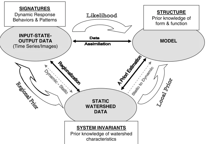
Signature-based evaluation enables the Bayesian infer-ence framework to be applied to the problem of prediction in ungaged basins, by exploiting three kinds of informa-tion about the system, namely:
1) Prior information about system form and function (summarized in the environmental Theory and expressed in the structure of the numerical model). 2) Prior information about system invariants (summarized
in the static system data —e.g. data about watershed characteristics—and expressed in the model parame-ters), and
3) New information about dynamic system response behaviours and patterns (summarized in the I-S-O data as time series and images of variations in system states and fluxes).
As expressed in Figure 6, the link from ‘I-S-O Data’ to ‘model’ represents the process of data assimilation which includes the steps of model identification, parameter estimation, and state estimation; an appropriate likelihood function (see previous section) is used to absorb relevant information in the data into the model.
The link from ‘static system data’ to ‘model’ represents the process ofa priori estimation in which static systems data (soils, vegetation, topography, geology, etc.) are used to specify the parameters (and possibly structure) of the model; this is based in the underlying Theory, while taking appropriate account of uncertainties in the data and in the theoretical relationships linking the data with the parameters (and model equations). For example, Koren et al. (2000) show how soils data can be linked to parameters of the Sacramento model used by the NWS for flood forecasting; similar approaches have been used elsewhere (Atkinsonet al., 2002; Ederet al., 2003; Farmeret al., 2003). The information in the static systems data is absorbed into the model by means of a local prior constructed via the data-to-parameters transformations while accounting for observational error.
INPUT-STATE-OUTPUT DATA
(Time Series/Images)
STATIC WATERSHED
DATA
MODEL SIGNATURES
Dynamic Response Behaviors & Patterns
SYSTEM INVARIANTS
Prior knowledge of watershed characteristics
STRUCTURE
Prior knowledge of form & function
Figure 6. The three kinds of information used to constrain the predictive model
related I-S-O signature behaviours seen in the dynamic systems data to indices extracted from the static system data; regionalization relationships were then constructed to predict the range of response behaviours expected in ungaged basins for which static system data were available. This regional information (expressed as a regional prior on the system responses) is then absorbed into the model as a regional prior that constrains the model parameters and structure.
Taken together, these three kinds of information— the signature-based likelihood, the local prior, and the signature-based regional prior— provide a strong basis for diagnostic model evaluation, a framework for recon-ciling environmental theory with data, and a procedure for constraining the uncertainty in numerical model pre-dictions.
SUMMARY AND CONCLUSIONS
Current strategies for confronting models with data are inadequate in the face of the highly complex and high order models that are central to modern environmental science, this model complexity being driven by soci-etal needs, increasing computational power, and the rapid pace of integration of eco-geo-hydro-meteorological pro-cess understanding. The need for improved approaches to model evaluation is well recognized by the scientific community both in the context of the international Pre-dictions in Ungaged Basins (PUB) initiative and in the NSF sponsored Environmental Observatories initiative in the USA, among others. We propose steps towards a robust and powerful ‘Theory of Evaluation’, which exploits the three ways in which model-to-system close-ness can be evaluated (a) by quantitative evaluation of behaviour, (b) qualitative evaluation of behaviour, and
(c) by qualitative evaluation of form and function. This paper discusses the need for a diagnostic approach to the model evaluation problem, rooted firmly in information theory and employing signature indices to measure the-oretically relevant system behaviours. By exploring the compressibility of the data, the approach can also help to identify the degree of system complexity resolvable by a model. Placed in the context of Bayesian uncer-tainty analysis, it can further be applied to the problem of prediction in ungaged basins.
These ideas are, in part, a formal re-working of infor-mal strategies for model identification that had been common practice in environmental science and modeling practice before resorting to statistical regression theory. As such, there exists a vast body of extant literature that can be mined for ways in which to define diag-nostically relevant (quantitative and qualitative) signature indices of system behaviour. There also exists virtually infinite scope for inventing new signature indices that are properly rooted in the relevant theory. Challenges lie in the (a) proper selection of the set of diagnostic measures (including type and number), (b) proper con-sideration of stochastic and other kinds of uncertainties, and (c) their assimilation into procedures for diagnosis and correction of model deficiencies. We suggest, how-ever, that proper application of environmental theory will tell us what kinds of signature patterns to expect (or look for) in the real world. Novel signature patterns observed in the data but not predicted to exist, or deviations in the form of observed signature patterns from those predicted, will suggest the existence of new information that must be assimilated to maintain a ‘good’ model. This atten-tion to signature patterns therefore constitutes the natural basis for diagnosis.
reconciliation. We believe that rapid progress can only be made through collaboration between experimental (field) scientists, theoretical scientists, modelers and systems theorists. It is particularly apparent in our view that a diagnostic evaluation approach must be rooted in the relevant environmental theory, and not solely in some generic systems- or statistical-based approach. In fact, it becomes the (partial) responsibility of the developers of the underlying theory/model to propose and demonstrate exactly how the proposed theory can be supported or falsified by recourse to observational processes. Further publications by the authors on the application of the diagnostic approach and related topics are forthcoming.
ACKNOWLEDGEMENTS
We gratefully acknowledge important conversations with Guillermo Martinez, Koray Yilmaz, Gab Abramowitz, Jeff McDonnell, Murugesu Sivapalan, John Schaake, Bruce Beck, Ross Woods, Martyn Clarke, Keith Beven, Peter Young, Patrick Reed, Victor Koren, Michael Smith, Pedro Restrepo, Jasper Vrugt, Kathryn van Werkhoven and many others that helped, in one way or another, to clarify many of the ideas presented here. Partial support for this work was provided by SAHRA (an NSF center for Sustainability of Semi-Arid Hydrology and Riparian Areas) under grant EAR-9876800 and by the Hydrology Laboratory of the National Weather Service [Grants NA87WHO582 and NA07WH0144].
REFERENCES
Atkinson S, Woods RA, Sivapalan M. 2002. Climate and landscape controls on water balance model complexity over changing time scales. Water Resources Research 38(12): 1314. DOI: 10Ð1029/2002WR001487, pp. 50Ð1– 50Ð17.
Beck MB. 1985. Structures, failure, inference and prediction. In
Identification and System Parameter Estimation, ed. by Barker MA, Young PC.Proceedings IFAC/IFORS 7th Symposium, Volume 2, York, UK; 1443– 1448.
Beck MB, Gupta HV, Rastetter E, Butler R, Edelson D, Graber H, Gross L, Harmon T, McLaughlin D, Paola C, et al. 2007. Grand challenges of the future for environmental modeling, White Paper, submitted to NSF.
Beven KJ. 2001. How far can we go in distributed hydrological modeling?Hydrology and Earth System Sciences 5(1): 1– 12. Beven KJ. 2006. A manifesto for the equifinality thesis. Journal of
Hydrology320(1-2): 18– 36. DOI:10Ð1016/j.jhydrol.2005Ð07Ð007. Beven KJ, Binley AM. 1992. The future of distributed models: model
calibration and uncertainty in prediction.Hydrological Processes 6: 279– 298.
Boyle DP, Gupta HV, Sorooshian S. 2001. Towards improved stream-flow forecasts: the value of semi-distributed modeling.Water Resources Research37(11): 2749– 2759.
Duan Q, Gupta VK, Sorooshian S. 1993. A shuffled complex evolution approach for effective and efficient global minimization. Journal of Optimization Theory and Applications76(3): 501– 521.
Eder G, Sivapalan M, Nachtnebel HP. 2003. Modeling of water balances in Alpine catchment through exploitation of emergent properties over changing time scales.Hydrological Processes 17: 2125– 2149. DOI: 10Ð1002/hyp.1325.
Edwards AWF. 1972. Likelihood. Cambridge: Cambridge University Press.
Evensen G. 1994. Sequential data assimilation with a nonlinear quasigeostrophic model using Monte Carlo methods to forecast error statistics.Journal of Geophysical Research99: 10143– 10162.
Farmer D, Sivapalan M, Jothityangkoon C. 2003. Climate, soil and vegetation controls upon the variability of water balance in temperate and semi-arid landscapes: Downward approach to hydrological prediction.Water Resources Research39(2): 1035. DOI: 10Ð1029/2001WR000328.
Friedrich G, Stumptner M, Wotawa F. 1999. Model-based diagnosis of hardware designs.Artificial Intelligence111: 3– 39.
Gall J. 1986.Systemantics : The Underground Text of Systems Lore, 2nd edn. General Systemantics Press.
Gordon N, Salmond D, Smith AFM. 1993. Novel approach to nonlinear and non-Gaussian Bayesian state estimation. Proceedings of the Institute Electrical Engineers F140: 107– 113.
Grayson R, Bl¨oschl G (eds) 2000. Spatial Patterns in Catchment Hydrology: Observations and Modelling. Cambridge University Press: Cambridge, ISBN 0-521-63316-8.
Gupta HV. 2000. The Devilish Dr. M or some comments on the identification of hydrologic models. In Proceedings of the Seventh Annual Meeting of the British Hydrological Society, Newcastle, UK. Gupta HV, Beven KJ, Wagener T. 2005. Model calibration and
uncertainty estimation. In Encyclopedia of Hydrological Sciences, Anderson MG,et al. (eds). John Wiley & Sons Ltd: Chichester; 1– 17. Gupta HV, Mahmoud M., Liu Y, Brookshire D, Coursey D, Broad-bent C. 2007. Management of water resources for an uncertain future: the role of scenario analysis in designing water markets. In Proceed-ings of the International Conference on Water, Environment, Energy and Society (WEES)-2007,National Institute of Hydrology: Roorkee, India; 18– 21.
Gupta VK, Sorooshian S. 1983. Uniqueness and observability of conceptual rainfall-runoff model parameters: The percolation process examined.Water Resources Research19(1): 269– 276.
Gupta HV, Sorooshian S, Yapo PO. 1998. Towards improved calibration of hydrologic models: multiple and non-commensurable measures of information.Water Resources Research34(4): 751– 763.
Hankerson DR, Harris GA, Johnson Jr. PD. 2003. Introduction to Information Theory and Data Compression, 2nd edn. CRC Press: Florida. ISBN 1-58488-313-8.
Illman WA, Neuman SP. 2001. Type curve interpretation of a cross-hole pneumatic injection test in unsaturated fractured tuff.Water Resources Research37: 583– 603.
Jakeman AJ, Hornberger GM. 1993. How much complexity is warranted in a rainfall-runoff model? Water Resources Research 29(8): 2637– 2649.
Johnston PR, Pilgrim DH. 1976. Parameter optimization for watershed models.Water Resources Research12(3): 477– 486.
Kalman RE. 1960. New approach to linear filtering and prediction problems.Journal Basic Engineering35– 64.
Koren VI, Smith M, Wang D, Zhang Z. 2000. Use of soil property data in the derivation of conceptual rainfall-runoff model parameters. In
Proceedings of the 15th Conference on Hydrology, AMS: Long Beach, CA; 103– 106.
Lin Z, Beck MB. 2007. On the identification of model structure in hydrological and environmental systems. Water Resources Research 43: W02402. DOI:1029/2005WR004796.
Liu Y, Gupta HV. 2007. Uncertainty in hydrological modeling: towards an integrated data assimilation framework.Water Resources Research 43: W07401. DOI:10Ð1029/2006WR005756.
Liu Y, Gupta HV, Springer E, Wagener T. 2007. Linking sci-ence with environmental decision making: experisci-ences from an integrated modeling approach to supporting sustainable water resources management. Environmental Modeling and Software
DOI:10Ð1016/j.envsoft.2007Ð10Ð007.
Moench A. 1994. Specific yield as determined by type-curve analysis of aquifer-test data.Ground Water 32: 949– 957.
Moradkhani H, Hsu KL, Gupta HV, Sorooshian S. 2005. Uncertainty assessment of hydrologic model states and parameters: Sequential data assimilation using the particle filter. Water Resources Research 41: W05012. DOI:10Ð1029/2004WR003604.
Oreskes N, Schrader-Frechette K, Belitz K. 1994. Verification, validation and confirmation of numerical models in the earth sciences.Science 263: 641– 646.
Peischl B, Wotawa F. 2003. Model-based diagnosis or reasoning from first principles.IEEE Intelligent Systems18: 32– 37.
Popper K. 2000. The Logic of Scientific Discovery. Hutchinson Education/Routledge: UK.
Reiter R. 1987. A theory of diagnosis from first principles. Artificial Intelligence32: 57– 95.
catchment, Water Resources Research 42: W06407, DOI:10Ð1029/ 2005WR004373.
Rupp DE, Selker JS. 2006. Information, artifacts, and noise in dQ/dt — Q recession analysis.Advances in Water Resources29(2): 154– 160. Saltelli A, Tarantola S, Campolongo F, Ratto M. 2004. Sensitivity
Analysis in Practice: A Guide to Assessing Scientific Models. John Wiley & Sons.
Saunders Jr EM. 1993. Stock prices and wallstreet weather. American Economic Revue83: 1337– 1345.
Schaeffli B, Gupta HV. 2007. Do Nash values have value?Hydrologic Processes 21(15): 2075– 2080. DOI: 10Ð1002/hyp.6825.
Seibert J. 2001. On the need for benchmarks in hydrological modeling.
Hydrological Processes15: 1063– 1064.
Seibert J, McDonnell JJ. 2002. On the dialog between experimentalist and modellers in catchment hydrology: use of soft data for multi-criteria model calibration. Water Resources Research 38(11): 1231– 1241.
Sivapalan M, Takeuchi K, Franks SW, Gupta VK, Karambiri H, Lakshmi V, Liang X, McDonnell JJ, Mendiondo EM, O’Connell PE,
et al. 2003a. IAHS decade on predictions in ungauged basins (PUB), 2003-2012: shaping an exciting future for the hydrological sciences.
Hydrological Sciences Journal48(6): 857– 880.
Sivapalan M, Bl¨oschl G, Zhang L, Vertessy R. 2003b. Downward approach to hydrological prediction. Hydrological Processes 17: 2101– 2111. DOI: 10Ð1002/hyp.1425.
Sorooshian S, Gupta VK. 1983. Automatic calibration of conceptual rainfall-runoff models: the question of parameter observability and uniqueness.Water Resources Research19(1): 260– 268.
Spear RC, Hornberger GM. 1980. Eutrophication in Peel Inlet-II: identification of critical uncertainties via generalized sensitivity analysis.Water Resources Research14(1): 43– 49.
Swartz MH. 2001. Textbook of Physical Diagnosis, History and Examination, 4th edn. Saunders: Philadelphia.
Thiemann M, Trosset M, Gupta HV, Sorooshian S. 2001. Bayesian recursive parameter estimation for hydrologic models.Water Resources Research37(10): 2521– 2535.
Trave-Massuyes L, Milne R. 1997. Gas-turbine condition monitoring using qualitative model-based diagnosis IEEEExpert12: 22– 31. Vogel RM, Fennessey NM. 1995. Flow duration curves. II. A review
of applications in water resource planning.Water Resources Bulletin 31(6): 1029– 1039.
Vogel RM, Sankarasubramanian A. 2003. The validation of a watershed model without calibration.Water Resources Research 39(10): 1292. DOI:10Ð1029/2002WR001940.
Vrugt JA, Gupta HV, Bastidas LA, Bouten W., Sorooshian S. 2003. Effective and efficient algorithm for multi-objective optimization of hydrologic models.Water Resources Research39(8): 5Ð1– 5Ð19. Wagener T. 2003. Evaluation of catchment models. Hydrological
Processes 17: 3375– 3378.
Wagener T, Gupta HV. 2005. Model identification for hydrological forecasting under uncertainty.Stochastic Environmental Research and Risk Assessment19(6): 378– 387. DOI: 10Ð1007/s00477-005-0006-5. Wagener T, McIntyre N. 2005. Identification of hydrologic models for
operational purposes.Hydrological Sciences Journal50(5): 1–18. Wagener T, Boyle DP, Lees MJ, Wheater HS, Gupta HV, Sorooshian S.
2001. A framework for development and application of hydrological models.Hydrology and Earth System Sciences5(1): 13– 26. Wagener T, McIntyre N, Lees MJ, Wheater HS, Gupta HV. 2003a.
Towards reduced uncertainty in conceptual rainfall-runoff modelling: Dynamic identifiability analysis. Hydrological Processes 17(2): 455– 476.
Wagener T, Freer J, Zehe E, Beven K, Gupta HV, Bardossy A. 2006. Towards an uncertainty framework for predictions in ungauged basins: the uncertainty working group. InPredictions in Ungauged Basins: Promise and Progress, Sivapalan M, Wagener T, Uhlenbrook S, Liang X, Lakshmi V, Kumar P, Zehe E, Tachikawa Y. (eds). IAHS Publication no. 303; 454– 462.
Wagener T, Sivapalan M, Troch P, Woods R. 2007. Catchment classifi-cation and hydrologic similarity.Geography Compass1(4): 901. DOI: 10Ð1111/j.1749Ð8198Ð2007Ð00039x.
Wagener T, Wheater HS, Gupta HV. 2003b. Identification and evaluation of watershed models. InCalibration of Watershed Models, Duan Q, Sorooshian S, Gupta HV, Rousseau A, Turcotte R (eds). AGU Monograph; 29– 47.
Yadav M, Wagener T, Gupta HV. 2007. Regionalization of constraints on expected watershed response behaviour for improved predictions in ungauged basins. Advances in Water Resources 30: 1756– 1774. DOI:10Ð1016/j.advwatres.2007Ð01Ð005.
Young PC. 2002. Advances in real-time flood forecasting.Philosophical Transactions of the Royal Society London A360: 1433– 1450. Young PC. 2003. Top-down and data-based mechanistic modelling of
rainfall-flow dynamics at the catchment scale.Hydrological Processes 17: 2195– 2217.