Fundamentals of
Electric Circuits
FiFt h Edition
f i f t h e d i t i o n
Fundamentals of
Electric Circuits
Charles K. Alexander
Department of Electrical and
Computer Engineering
Cleveland State University
Matthew N. O. Sadiku
Department of
Electrical Engineering
Prairie View A&M University
FUNDAMENTALS OF ELECTRIC CIRCUITS, FIFTH EDITION
Published by McGraw-Hill, a business unit of The McGraw-Hill Companies, Inc., 1221 Avenue of the Americas, New York, NY 10020. Copyright © 2013 by The McGraw-Hill Companies, Inc. All rights reserved. Printed in the United States of America. Previous editions © 2009, 2007 and 2004. No part of this publication may be reproduced or distributed in any form or by any means, or stored in a database or retrieval system, without the prior written consent of The McGraw-Hill Companies, Inc., including, but not limited to, in any network or other electronic storage or transmission, or broadcast for distance learning.
Some ancillaries, including electronic and print components, may not be available to customers outside the United States.
This book is printed on acid-free paper.
1 2 3 4 5 6 7 8 9 0 RJE/RJE 1 0 9 8 7 6 5 4 3 2 ISBN 978-0-07-338057-5
MHID 0-07-338057-1
Vice President & Editor-in-Chief: Marty Lange
Vice President & Director of Specialized Publishing: Janice M. Roerig-Blong
Editorial Director: Michael Lange
Publisher: Raghothaman Srinivasan
Marketing Manager: Curt Reynolds
Developmental Editor: Lora Neyens
Project Manager: Joyce Watters/Lisa Bruflodt
Design Coordinator: Margarite Reynolds
Cover Designer: Studio Montage, St. Louis, Missouri
Cover Image Credit: NASA. Artist’s Concept of Rover on Mars
Buyer: Sherry L. Kane
Media Project Manager: Balaji Sundararaman
Compositor: MPS Limited, a Macmillan Company
Typeface: 10/12 Times Roman
Printer: RR Donnelly
All credits appearing on page or at the end of the book are considered to be an extension of the copyright page.
Library of Congress Cataloging-in-Publication Data
Alexander, Charles K.
Fundamentals of electric circuits / Charles K. Alexander, Matthew N. O. Sadiku. — 5th ed. p. cm.
ISBN 978-0-07-338057-5 (alk. paper)
1. Electric circuits. I. Sadiku, Matthew N. O. II. Title. TK454.A452 2012
621.319'24—dc23 2011025116
www.mhhe.com
Dedicated to our wives, Kikelomo and Hannah, whose understanding and
support have truly made this book possible.
Contents
Preface xi
Acknowledgements xvi A Note to the Student xix About the Authors xxi
PART 1 DC Circuits 2
Chapter 1 Basic Concepts 3
1.1 Introduction 4
1.2 Systems of Units 5
1.3 Charge and Current 5
1.4 Voltage 9
1.5 Power and Energy 10
1.6 Circuit Elements 15
1.7 †Applications 17
1.7.1 TV Picture Tube 1.7.2 Electricity Bills
1.8 †Problem Solving 20
1.9 Summary 23
Review Questions 24 Problems 24
Comprehensive Problems 27
Chapter 2 Basic Laws 29
2.1 Introduction 30
2.2 Ohm’s Law 30
2.3 †Nodes, Branches, and Loops 35 2.4 Kirchhoff’s Laws 37
2.5 Series Resistors and Voltage Division 43 2.6 Parallel Resistors and Current Division 45 2.7 †Wye-Delta Transformations 52
Delta to Wye Conversion Wye to Delta Conversion
2.8 †Applications 58
2.8.1 Lighting Systems 2.8.2 Design of DC Meters
2.9 Summary 64
Review Questions 66 Problems 67
Comprehensive Problems 78
v Chapter 3 Methods of Analysis 81
3.1 Introduction 82
3.2 Nodal Analysis 82
3.3 Nodal Analysis with Voltage
Sources 88
3.4 Mesh Analysis 93
3.5 Mesh Analysis with Current Sources 98 3.6 †Nodal and Mesh Analyses
by Inspection 100
3.7 Nodal Versus Mesh Analysis 104 3.8 Circuit Analysis with PSpice 105 3.9 †Applications: DC Transistor
Circuits 107
3.10 Summary 112
Review Questions 113 Problems 114
Comprehensive Problem 126
Chapter 4 Circuit Theorems 127
4.1 Introduction 128
4.2 Linearity Property 128
4.3 Superposition 130
4.4 Source Transformation 135
4.5 Thevenin’s Theorem 139
4.6 Norton’s Theorem 145
4.7 †Derivations of Thevenin’s and Norton’s Theorems 149
4.8 Maximum Power Transfer 150
4.9 Verifying Circuit Theorems with PSpice 152 4.10 †Applications 155
4.10.1 Source Modeling 4.10.2 Resistance Measurement
4.11 Summary 160
Review Questions 161 Problems 162
Comprehensive Problems 173
Chapter 5 Operational Amplifiers 175
5.1 Introduction 176
vi Contents
5.3 Ideal Op Amp 179
5.4 Inverting Amplifier 181 5.5 Noninverting Amplifier 183
5.6 Summing Amplifier 185
5.7 Difference Amplifier 187
5.8 Cascaded Op Amp Circuits 191
5.9 Op Amp Circuit Analysis with PSpice 194 5.10 †Applications 196
5.10.1 Digital-to-Analog Converter 5.10.2 Instrumentation Amplifiers
5.11 Summary 199
Review Questions 201 Problems 202
Comprehensive Problems 213
Chapter 6 Capacitors and Inductors 215
6.1 Introduction 216
6.2 Capacitors 216
6.3 Series and Parallel Capacitors 222
6.4 Inductors 226
6.5 Series and Parallel Inductors 230
6.6 †Applications 233
6.6.1 Integrator 6.6.2 Differentiator 6.6.3 Analog Computer
6.7 Summary 240
Review Questions 241 Problems 242
Comprehensive Problems 251
Chapter 7 First-Order Circuits 253
7.1 Introduction 254
7.2 The Source-Free RCCircuit 254 7.3 The Source-Free RLCircuit 259 7.4 Singularity Functions 265
7.5 Step Response of an RCCircuit 273 7.6 Step Response of an RLCircuit 280 7.7 †First-Order Op Amp Circuits 284 7.8 Transient Analysis with PSpice 289
7.9 †Applications 293
7.9.1 Delay Circuits 7.9.2 Photoflash Unit 7.9.3 Relay Circuits
7.9.4 Automobile Ignition Circuit
7.10 Summary 299
Review Questions 300 Problems 301
Comprehensive Problems 311
Chapter 8 Second-Order Circuits 313
8.1 Introduction 314
8.2 Finding Initial and Final Values 314 8.3 The Source-Free Series
RLCCircuit 319 8.4 The Source-Free Parallel
RLCCircuit 326
8.5 Step Response of a Series RLC Circuit 331
8.6 Step Response of a ParallelRLC Circuit 336
8.7 General Second-Order Circuits 339
8.8 Second-Order Op Amp Circuits 344
8.9 PSpiceAnalysis of RLCCircuits 346 8.10 †Duality 350
8.11 †Applications 353
8.11.1 Automobile Ignition System 8.11.2 Smoothing Circuits
8.12 Summary 356
Review Questions 357 Problems 358
Comprehensive Problems 367
PART 2 AC Circuits 368
Chapter 9 Sinusoids and Phasors 369
9.1 Introduction 370
9.2 Sinusoids 371
9.3 Phasors 376
9.4 Phasor Relationships for Circuit Elements 385
9.5 Impedance and Admittance 387
9.6 †Kirchhoff’s Laws in the Frequency
Domain 389
9.7 Impedance Combinations 390
9.8 †Applications 396
9.8.1 Phase-Shifters 9.8.2 AC Bridges
9.9 Summary 402
Review Questions 403 Problems 403
Comprehensive Problems 411
Chapter 10 Sinusoidal Steady-State Analysis 413
10.1 Introduction 414 10.2 Nodal Analysis 414
Contents vii
12.11 Summary 543
Review Questions 543 Problems 544
Comprehensive Problems 553
Chapter 13 Magnetically Coupled Circuits 555
13.1 Introduction 556 13.2 Mutual Inductance 556
13.3 Energy in a Coupled Circuit 564 13.4 Linear Transformers 567 13.5 Ideal Transformers 573 13.6 Ideal Autotransformers 581 13.7 †Three-Phase Transformers 584 13.8 PSpiceAnalysis of Magnetically
Coupled Circuits 586 13.9 †Applications 591
13.9.1 Transformer as an Isolation Device 13.9.2 Transformer as a Matching Device 13.9.3 Power Distribution
13.10 Summary 597
Review Questions 598 Problems 599
Comprehensive Problems 611
Chapter 14 Frequency Response 613
14.1 Introduction 614 14.2 Transfer Function 614 14.3 †The Decibel Scale 617
14.4 Bode Plots 619
14.5 Series Resonance 629 14.6 Parallel Resonance 634 14.7 Passive Filters 637
14.7.1 Lowpass Filter 14.7.2 Highpass Filter 14.7.3 Bandpass Filter 14.7.4 Bandstop Filter
14.8 Active Filters 642
14.8.1 First-Order Lowpass Filter 14.8.2 First-Order Highpass Filter 14.8.3 Bandpass Filter
14.8.4 Bandreject (or Notch) Filter
14.9 Scaling 648
14.9.1 Magnitude Scaling 14.9.2 Frequency Scaling
14.9.3 Magnitude and Frequency Scaling
14.10 Frequency Response Using PSpice 652
14.11 Computation Using MATLAB 655
10.4 Superposition Theorem 421
10.5 Source Transformation 424 10.6 Thevenin and Norton
Equivalent Circuits 426
10.7 Op Amp AC Circuits 431
10.8 AC Analysis Using PSpice 433 10.9 †Applications 437
10.9.1 Capacitance Multiplier 10.9.2 Oscillators
10.10 Summary 441
Review Questions 441 Problems 443
Chapter 11 AC Power Analysis 457
11.1 Introduction 458
11.2 Instantaneous and Average
Power 458
11.3 Maximum Average Power
Transfer 464
11.4 Effective or RMS Value 467 11.5 Apparent Power and
Power Factor 470
11.6 Complex Power 473
11.7 †Conservation of AC Power 477 11.8 Power Factor Correction 481 11.9 †Applications 483
11.9.1 Power Measurement 11.9.2 Electricity Consumption Cost
11.10 Summary 488
Review Questions 490 Problems 490
Comprehensive Problems 500
Chapter 12 Three-Phase Circuits 503
12.1 Introduction 504
12.2 Balanced Three-Phase Voltages 505
12.3 Balanced Wye-Wye Connection 509
12.4 Balanced Wye-Delta Connection 512 12.5 Balanced Delta-Delta
Connection 514
12.6 Balanced Delta-Wye Connection 516 12.7 Power in a Balanced System 519 12.8 †Unbalanced Three-Phase
Systems 525
12.9 PSpicefor Three-Phase Circuits 529 12.10 †Applications 534
viii Contents
14.12 †Applications 657
14.12.1 Radio Receiver 14.12.2 Touch-Tone Telephone 14.12.3 Crossover Network
14.13 Summary 663
Review Questions 664 Problems 665
Comprehensive Problems 673
PART 3 Advanced Circuit Analysis 674
Chapter 15 Introduction to the Laplace Transform 675
15.1 Introduction 676
15.2 Definition of the Laplace Transform 677 15.3 Properties of the Laplace Transform 679 15.4 The Inverse Laplace Transform 690
15.4.1 Simple Poles 15.4.2 Repeated Poles 15.4.3 Complex Poles
15.5 The Convolution Integral 697 15.6 †Application to Integrodifferential
Equations 705
15.7 Summary 708
Review Questions 708 Problems 709
Chapter 16 Applications of the Laplace Transform 715
16.1 Introduction 716
16.2 Circuit Element Models 716 16.3 Circuit Analysis 722 16.4 Transfer Functions 726 16.5 State Variables 730 16.6 †Applications 737
16.6.1 Network Stability 16.6.2 Network Synthesis
16.7 Summary 745
Review Questions 746 Problems 747
Comprehensive Problems 758
Chapter 17 The Fourier Series 759
17.1 Introduction 760
17.2 Trigonometric Fourier Series 760
17.3 Symmetry Considerations 768
17.3.1 Even Symmetry 17.3.2 Odd Symmetry 17.3.3 Half-Wave Symmetry
17.4 Circuit Applications 778
17.5 Average Power and RMS Values 782
17.6 Exponential Fourier Series 785 17.7 Fourier Analysis with PSpice 791
17.7.1 Discrete Fourier Transform 17.7.2 Fast Fourier Transform
17.8 †Applications 797 17.8.1 Spectrum Analyzers 17.8.2 Filters
17.9 Summary 800
Review Questions 802 Problems 802
Comprehensive Problems 811
Chapter 18 Fourier Transform 813
18.1 Introduction 814
18.2 Definition of the Fourier Transform 814 18.3 Properties of the Fourier
Transform 820
18.4 Circuit Applications 833 18.5 Parseval’s Theorem 836 18.6 Comparing the Fourier and
Laplace Transforms 839 18.7 †Applications 840
18.7.1 Amplitude Modulation 18.7.2 Sampling
18.8 Summary 843
Review Questions 844 Problems 845
Comprehensive Problems 851
Chapter 19 Two-Port Networks 853
19.1 Introduction 854
19.2 Impedance Parameters 854
19.3 Admittance Parameters 859 19.4 Hybrid Parameters 862 19.5 Transmission Parameters 867 19.6 †Relationships Between
Parameters 872
19.7 Interconnection of Networks 875 19.8 Computing Two-Port Parameters
Using PSpice 881 19.9 †Applications 884
Contents ix
19.10 Summary 893
Review Questions 894 Problems 894
Comprehensive Problem 905
Appendix A Simultaneous Equations and Matrix Inversion A
Appendix B Complex Numbers A-9
Appendix C Mathematical Formulas A-16
Appendix D Answers to Odd-Numbered Problems A-21
xi
Preface
You may be wondering why we chose a photo of NASA’s Mars Rover for the cover. We actually chose it for several reasons. Obviously, it is very exciting; in fact, space represents the most exciting frontier for the entire world! In addition, much of the Rover itself consists of all kinds of circuits. Circuits that must work without needing maintenance! Once you are on Mars, it is hard to find a technician!
The Rover must have a power system that can supply all the power necessary to move it, help it collect samples and analyze them, broadcast the results back to Earth, and receive instructions from Earth. One of the important issues that make the problem of working with the rover is that it takes about 20 minutes for communications to go from the Earth to Mars. So the Rover does not make changes required by NASA quickly.
What we find most amazing is that such a sophisticated and com-plicated electro-mechanical device can operate so accurately and reli-ably after flying millions of miles and being bounced onto the ground! Here is a link to an absolutely incredible video of what the Rover is all about and how it got to Mars: http://www.youtube.com/ watch?v=5UmRx4dEdRI. Enjoy!
Features
New to This Edition
A model for magnetic coupling is presented in Chapter 13 that will make analysis easier as well as enhance your ability to find errors. We have suc-cessfully used this model for years and felt it was now time to add it to the book. In addition, there are over 600 new end-of-chapter problems, changed end-of-chapter problems, and changed practice problems.
We have also added National Instruments MultisimTMsolutions for almost all of the problems solved using PSpice®. There is a Multisim
tutorial available on our website. We have added National Instruments
Multisim since it is very user-friendly with many more options for analysis than PSpice. In addition, it allows the ability to modify circuits easily in order to see how changing circuit parameters impacts voltages, currents, and power. We have also moved the tutorials for PSpice, MAT-LAB®,andKCIDEto our website to allow us to keep up with changes in the software.
We have also added 43 new problems to Chapter 16. We did this to enhance using the powerful s-domain analysis techniques to finding voltages and currents in circuits.
Retained from Previous Editions
xii Preface
An important part of this book is our 121 design a problemproblems. These problems were developed to enhance skills that are an important part of the design process. We know it is not possible to fully develop a student’s design skills in a fundamental course like circuits. To fully develop design skills a student needs a design experience normally reserved for their senior year. This does not mean that some of those skills cannot be developed and exercised in a circuits course. The text already included open-ended questions that help students use creativ-ity, which is an important part of learning how to design. We already have some questions that are open-ended but we desired to add much more into our text in this important area and have developed an approach to do just that. When we develop problems for the student to solve our goal is that in solving the problem the student learns more about the theory and the problem solving process. Why not have the students design problems like we do? That is exactly what we do in each chapter. Within the normal problem set, we have a set of prob-lems where we ask the student to design a problem to help other stu-dents better understand an important concept. This has two very important results. The first will be a better understanding of the basic theory and the second will be the enhancement of some of the student’s basic design skills. We are making effective use of the principle of learning by teaching. Essentially we all learn better when we teach a subject. Designing effective problems is a key part of the teaching process. Students should also be encouraged to develop problems, when appropriate, which have nice numbers and do not necessarily overemphasize complicated mathematical manipulations.
A very important advantage to our textbook, we have a total of 2,447 Examples, Practice Problems, Review Questions, and End-of-Chapter Problems! Answers are provided for all practice problems and the odd numbered end-of-chapter problems.
The main objective of the fifth edition of this book remains the same as the previous editions—to present circuit analysis in a manner that is clearer, more interesting, and easier to understand than other cir-cuit textbooks, and to assist the student in beginning to see the “fun” in engineering. This objective is achieved in the following ways:
• Chapter Openers and Summaries
Each chapter opens with a discussion about how to enhance skills which contribute to successful problem solving as well as success-ful careers or a career-oriented talk on a sub-discipline of electri-cal engineering. This is followed by an introduction that links the chapter with the previous chapters and states the chapter objectives. The chapter ends with a summary of key points and formulas. • Problem-Solving Methodology
Chapter 1 introduces a six-step method for solving circuit prob-lems which is used consistently throughout the book and media supplements to promote best-practice problem-solving procedures. • Student-Friendly Writing Style
Preface xiii
• Boxed Formulas and Key Terms
Important formulas are boxed as a means of helping students sort out what is essential from what is not. Also, to ensure that students clearly understand the key elements of the subject matter, key terms are defined and highlighted.
• Margin Notes
Marginal notes are used as a pedagogical aid. They serve multiple uses such as hints, cross-references, more exposition, warnings, reminders not to make some particular common mistakes, and problem-solving insights.
• Worked Examples
Thoroughly worked examples are liberally given at the end of every section. The examples are regarded as a part of the text and are clearly explained without asking the reader to fill in missing steps. Thoroughly worked examples give students a good under-standing of the solution process and the confidence to solve prob-lems themselves. Some of the probprob-lems are solved in two or three different ways to facilitate a substantial comprehension of the sub-ject material as well as a comparison of different approaches. • Practice Problems
To give students practice opportunity, each illustrative example is immediately followed by a practice problem with the answer. The student can follow the example step-by-step to aid in the solution of the practice problem without flipping pages or looking at the end of the book for answers. The practice problem is also intended to test a student’s understanding of the preceding example. It will reinforce their grasp of the material before the student can move on to the next section. Complete solutions to the practice problems are available to students on the website.
• Application Sections
The last section in each chapter is devoted to practical application aspects of the concepts covered in the chapter. The material cov-ered in the chapter is applied to at least one or two practical prob-lems or devices. This helps students see how the concepts are applied to real-life situations.
• Review Questions
Ten review questions in the form of multiple-choice objective items are provided at the end of each chapter with answers. The review questions are intended to cover the little “tricks” that the examples and end-of-chapter problems may not cover. They serve as a self test device and help students determine how well they have mastered the chapter.
• Computer Tools
• Design a Problem Problems
Finally, design a problem problems are meant to help the student develop skills that will be needed in the design process.
• Historical Tidbits
Historical sketches throughout the text provide profiles of impor-tant pioneers and events relevant to the study of electrical engineering.
• Early Op Amp Discussion
The operational amplifier (op amp) as a basic element is introduced early in the text.
• Fourier and Laplace Transforms Coverage
To ease the transition between the circuit course and signals and systems courses, Fourier and Laplace transforms are covered lucidly and thoroughly. The chapters are developed in a manner that the interested instructor can go from solutions of first-order circuits to Chapter 15. This then allows a very natural progression from Laplace to Fourier to AC.
• Four Color Art Program
An interior design and four color art program bring circuit drawings to life and enhance key pedagogical elements throughout the text. • Extended Examples
Examples worked in detail according to the six-step problem solv-ing method provide a roadmap for students to solve problems in a consistent fashion. At least one example in each chapter is devel-oped in this manner.
• EC 2000 Chapter Openers
Based on ABET’s skill-based CRITERION 3, these chapter open-ers are devoted to discussions as to how students can acquire the skills that will lead to a significantly enhanced career as an engi-neer. Because these skills are so very important to the student while still in college as well after graduation, we use the heading,
“Enhancing your Skills and your Career.”
• Homework Problems
There are 468 new or changed end-of-chapter problems which will provide students with plenty of practice as well as reinforce key concepts.
• Homework Problem Icons
Icons are used to highlight problems that relate to engineering design as well as problems that can be solved using PSpice, Mul-tisim, KCIDE, or MATLAB.
Organization
This book was written for a two-semester or three-quarter course in linear circuit analysis. The book may also be used for a one-semester course by a proper selection of chapters and sections by the instructor. It is broadly divided into three parts.
• Part 1, consisting of Chapters 1 to 8, is devoted to dc circuits. It covers the fundamental laws and theorems, circuits techniques, and passive and active elements.
Preface xv
• Part 2, which contains Chapter 9 to 14, deals with ac circuits. It introduces phasors, sinusoidal steady-state analysis, ac power, rms values, three-phase systems, and frequency response.
• Part 3, consisting of Chapters 15 to 19, are devoted to advanced techniques for network analysis. It provides students with a solid introduction to the Laplace transform, Fourier series, Fourier trans-form, and two-port network analysis.
The material in the three parts is more than sufficient for a two-semester course, so the instructor must select which chapters or sections to cover. Sections marked with the dagger sign (†) may be skipped, explained briefly, or assigned as homework. They can be omitted without loss of continuity. Each chapter has plenty of problems grouped according to the sections of the related material and diverse enough that the instruc-tor can choose some as examples and assign some as homework. As stated earlier, we are using three icons with this edition. We are using to denote problems that either require PSpice in the solution process, where the circuit complexity is such that PSpiceor Multisim
would make the solution process easier, and where PSpiceor Multisim
makes a good check to see if the problem has been solved correctly. We are using to denote problems where MATLABis required in the solution process, where MATLABmakes sense because of the problem makeup and its complexity, and where MATLAB makes a good check to see if the problem has been solved correctly. Finally, we use to identify problems that help the student develop skills that are needed for engineering design. More difficult problems are marked with an asterisk (*).
Comprehensive problems follow the end-of-chapter problems. They are mostly applications problems that require skills learned from that particular chapter.
Prerequisites
As with most introductory circuit courses, the main prerequisites, for a course using this textbook, are physics and calculus. Although famil-iarity with complex numbers is helpful in the later part of the book, it is not required. A very important asset of this text is that ALL the math-ematical equations and fundamentals of physics needed by the student, are included in the text.
Supplements
McGraw-Hill Connect
®Engineering
xvi Preface
Instructor and Student Website
Available at www.mhhe.com/alexander are a number of additional instructor and student resources to accompany the text. These include complete solutions for all practice and end-of-chapter problems, solu-tions in PSpice and Multisim problems, lecture PowerPoints®, text image files, transition guides to instructors, Network Analysis Tutori-als, FE Exam questions, flashcards, and primers for PSpice, Multisim, MATLAB, and KCIDE. The site also features COSMOS, a complete online solutions manual organization system that allows instructors to create custom homework, quizzes, and tests using end-of-chapter prob-lems from the text.
Knowledge Capturing Integrated Design
Environment for Circuits (KCIDE for Circuits)
This software, developed at Cleveland State University and funded by NASA, is designed to help the student work through a circuits problem in an organized manner using the six-step problem-solving methodol-ogy in the text. KCIDE for Circuitsallows students to work a circuit problem in PSpice and MATLAB, track the evolution of their solution, and save a record of their process for future reference. In addition, the software automatically generates a Word document and/or a PowerPoint presentation. The software package can be downloaded for free.
It is hoped that the book and supplemental materials supply the instructor with all the pedagogical tools necessary to effectively pres-ent the material.
McGraw-Hill Create™
Craft your teaching resources to match the way you teach! With McGraw-Hill Create, www.mcgrawhillcreate.com, you can easily rearrange chapters, combine material from other content sources, and quickly upload content you have written like your course syllabus or teaching notes. Find the content you need in Create by searching through thousands of leading McGraw-Hill textbooks. Arrange your book to fit your teaching style. Create even allows you to personalize your book’s appearance by selecting the cover and adding your name, school, and course information. Order a Create book and you’ll receive a complimentary print review copy in three to five business days or a complimentary electronic review copy (eComp) via e-mail in minutes. Go to www.mcgrawhillcreate.com today and register to experience how McGraw-Hill Create empowers you to teach yourstudents yourway.
Acknowledgements
Preface xvii
At McGraw-Hill, we would like to thank the following editorial and production staff: Raghu Srinivasan, publisher and senior sponsoring editor; Lora Kalb-Neyens, developmental editor; Curt Reynolds, marketing manager, Joyce Watters, project manager; and Margarite Reynolds, designer.
The fifth edition has benefited greatly from the many outstanding reviewers and symposium attendees who contributed to the success of the first four editions! In addition, the following have made important contributions to this edition (in alphabetical order):
Alok Berry, George Mason University
Vahe Caliskan, University of Illinois-Chicago
Archie Holmes, University of Virginia
Anton Kruger, University of Iowa
Arnost Neugroschel, University of Florida
Arun Ravindran, University of North Carolina-Charlotte
Finally, we appreciate the feedback received from instructors and students who used the previous editions. We want this to continue, so please keep sending us e-mails or direct them to the publisher. We can be reached at [email protected] for Charles Alexander and [email protected] for Matthew Sadiku.
A Note to the Student
This may be your first course in electrical engineering. Although elec-trical engineering is an exciting and challenging discipline, the course may intimidate you. This book was written to prevent that. A good text-book and a good professor are an advantage—but you are the one who does the learning. If you keep the following ideas in mind, you will do very well in this course.
• This course is the foundation on which most other courses in the electrical engineering curriculum rest. For this reason, put in as much effort as you can. Study the course regularly.
• Problem solving is an essential part of the learning process. Solve as many problems as you can. Begin by solving the practice problem following each example, and then proceed to the end-of-chapter prob-lems. The best way to learn is to solve a lot of probprob-lems. An aster-isk in front of a problem indicates a challenging problem.
• Spice and Multisim, computer circuit analysis programs, are used throughout the textbook. PSpice, the personal computer version of
Spice, is the popular standard circuit analysis program at most uni-versities. PSpice for Windowsand Multisim are described on our website. Make an effort to learn PSpiceand/or Multisim, because you can check any circuit problem with them and be sure you are handing in a correct problem solution.
• MATLABis another software that is very useful in circuit analysis and other courses you will be taking. A brief tutorial on MATLAB
can be found on our website. The best way to learn MATLAB is to start working with it once you know a few commands. • Each chapter ends with a section on how the material covered in
the chapter can be applied to real-life situations. The concepts in this section may be new and advanced to you. No doubt, you will learn more of the details in other courses. We are mainly interested in gaining a general familiarity with these ideas.
• Attempt the review questions at the end of each chapter. They will help you discover some “tricks” not revealed in class or in the textbook.
• Clearly a lot of effort has gone into making the technical details in this book easy to understand. It also contains all the mathematics and physics necessary to understand the theory and will be very useful in your other engineering courses. However, we have also focused on creating a reference for you to use both in school as well as when working in industry or seeking a graduate degree. • It is very tempting to sell your book after you have completed your
classroom experience; however, our advice to you is DO NOT SELL YOUR ENGINEERING BOOKS! Books have always been expen-sive; however, the cost of this book is virtually the same as I paid for my circuits text back in the early 60s in terms of real dollars. In
fact, it is actually cheaper. In addition, engineering books of the past are nowhere near as complete as what is available now.
When I was a student, I did not sell any of my engineering text-books and was very glad I did not! I found that I needed most of them throughout my career.
A short review on finding determinants is covered in Appendix A, complex numbers in Appendix B, and mathematical formulas in Appen-dix C. Answers to odd-numbered problems are given in AppenAppen-dix D.
Have fun!
C. K. A. and M. N. O. S.
xxi
About the Authors
Charles K. Alexander is professor of electrical and computer engi-neering in the Fenn College of Engiengi-neering at Cleveland State Uni-versity, Cleveland, Ohio. He is also the Director of The Center for Research in Electronics and Aerospace Technology (CREATE). From 2002 until 2006 he was Dean of the Fenn College of Engineering. From 2004 until 2007, he was Director of Ohio ICE, a research center in instrumentation, controls, electronics, and sensors (a coalition of CSU, Case, the University of Akron, and a number of Ohio industries). From 1998 until 2002, he was interim director (2000 and 2001) of the Insti-tute for Corrosion and Multiphase Technologies and Stocker Visiting Professor of electrical engineering and computer science at Ohio Uni-versity. From 1994–1996 he was dean of engineering and computer science at California State University, Northridge.
From 1989–1994 he was acting dean of the college of engineer-ing at Temple University, and from 1986–1989 he was professor and chairman of the department of electrical engineering at Temple. From 1980–1986 he held the same positions at Tennessee Technological Uni-versity. He was an associate professor and a professor of electrical engineering at Youngstown State University from 1972–1980, where he was named Distinguished Professor in 1977 in recognition of “out-standing teaching and research.” He was assistant professor of electri-cal engineering at Ohio University in 1971–1972. He received honorary Dr. Eng. from Ohio Northern University (2009), the PhD (1971) and M.S.E.E. (1967) from Ohio University and the B.S.E.E. (1965) from Ohio Northern University.
Dr. Alexander has been a consultant to 23 companies and gov-ernmental organizations, including the Air Force and Navy and sev-eral law firms. He has received over $85 million in research and development funds for projects ranging from solar energy to software engineering. He has authored 40 publications, including a workbook and a videotape lecture series, and is coauthor of Fundamentals of Electric Circuits, Problem Solving Made Almost Easy, and the fifth edition of the Standard Handbook of Electronic Engineering, with McGraw-Hill. He has made more than 500 paper, professional, and technical presentations.
Dr. Alexander is a fellow of the IEEE and served as its president and CEO in 1997. In 1993 and 1994 he was IEEE vice president, pro-fessional activities, and chair of the United States Activities Board (USAB). In 1991–1992 he was region 2 director, serving on the Regional Activities Board (RAB) and USAB. He has also been a mem-ber of the Educational Activities Board. He served as chair of the USAB Member Activities Council and vice chair of the USAB Professional Activities Council for Engineers, and he chaired the RAB Student Activities Committee and the USAB Student Professional Awareness Committee.
In 1998 he received the Distinguished Engineering Education Achievement Award from the Engineering Council, and in 1996 he received the Distinguished Engineering Education Leadership Award from the same group. When he became a fellow of the IEEE in 1994, the citation read “for leadership in the field of engineering education and the professional development of engineering students.” In 1984 he received the IEEE Centennial Medal, and in 1983 he received the IEEE/RAB Innovation Award, given to the IEEE member who best con-tributes to RAB’s goals and objectives.
Matthew N. O. Sadiku is presently a professor at Prairie View A&M University. Prior to joining Prairie View, he taught at Florida Atlantic University, Boca Raton, and Temple University, Philadelphia. He has also worked for Lucent/Avaya and Boeing Satellite Systems.
Dr. Sadiku is the author of over 170 professional papers and almost 30 books including Elements of Electromagnetics (Oxford University Press, 3rd ed., 2001), Numerical Techniques in Electromagnetics(2nd ed., CRC Press, 2000), Simulation of Local Area Networks (with M. IIyas, CRC Press, 1994), Metropolitan Area Networks(CRC Press, 1994), and
Fundamentals of Electric Circuits(with C. K. Alexander, McGraw-Hill). His books are used worldwide, and some of them have been translated into Korean, Chinese, Italian, and Spanish. He was the recipient of the 2000 McGraw-Hill/Jacob Millman Award for outstanding contributions in the field of electrical engineering. He was the IEEE region 2 Student Activities Committee chairman and is an associate editor for IEEE “Transactions on Education.” He received his PhD at Tennessee Technological University, Cookeville.
xxii About the Authors
Fundamentals of
P A R T O N E
DC Circuits
OUTLINE
1
Basic Concepts
2
Basic Laws
3
Methods of Analysis
4
Circuit Theorems
5
Operational Amplifiers
6
Capacitors and Inductors
7
First-Order Circuits
8
Second-Order Circuits
3
Basic Concepts
Some books are to be tasted, others to be swallowed, and some few to be chewed and digested.
—Francis Bacon
c h a p t e r
1
Enhancing Your Skills and Your Career
ABET EC 2000 criteria (3.a), “an ability to apply knowledge
of mathematics, science, and engineering.”
As students, you are required to study mathematics, science, and engi-neering with the purpose of being able to apply that knowledge to the solution of engineering problems. The skill here is the ability to apply the fundamentals of these areas in the solution of a problem. So how do you develop and enhance this skill?
The best approach is to work as many problems as possible in all of your courses. However, if you are really going to be successful with this, you must spend time analyzing where and when and why you have difficulty in easily arriving at successful solutions. You may be sur-prised to learn that most of your problem-solving problems are with mathematics rather than your understanding of theory. You may also learn that you start working the problem too soon. Taking time to think about the problem and how you should solve it will always save you time and frustration in the end.
What I have found that works best for me is to apply our six-step problem-solving technique. Then I carefully identify the areas where I have difficulty solving the problem. Many times, my actual deficiencies are in my understanding and ability to use correctly cer-tain mathematical principles. I then return to my fundamental math texts and carefully review the appropriate sections, and in some cases, work some example problems in that text. This brings me to another important thing you should always do: Keep nearby all your basic mathematics, science, and engineering textbooks.
This process of continually looking up material you thought you had acquired in earlier courses may seem very tedious at first; how-ever, as your skills develop and your knowledge increases, this process will become easier and easier. On a personal note, it is this very process that led me from being a much less than average student to someone who could earn a Ph.D. and become a successful researcher.
4 Chapter 1 Basic Concepts
+
−
Current
Lamp Battery
Figure 1.1
A simple electric circuit.
L1
C4
Antenna
C5
Q2
R7
R2 R4 R6
R3 R5
C1
C3
C2
Electret microphone
R1
+
−
+ 9 V (DC)
Q1
Figure 1.2
Electric circuit of a radio transmitter.
Introduction
Electric circuit theory and electromagnetic theory are the two funda-mental theories upon which all branches of electrical engineering are built. Many branches of electrical engineering, such as power, electric machines, control, electronics, communications, and instrumentation, are based on electric circuit theory. Therefore, the basic electric circuit theory course is the most important course for an electrical engineer-ing student, and always an excellent startengineer-ing point for a beginnengineer-ing stu-dent in electrical engineering education. Circuit theory is also valuable to students specializing in other branches of the physical sciences because circuits are a good model for the study of energy systems in general, and because of the applied mathematics, physics, and topol-ogy involved.
In electrical engineering, we are often interested in communicating or transferring energy from one point to another. To do this requires an interconnection of electrical devices. Such interconnection is referred to as an electric circuit, and each component of the circuit is known as an element.
An electric circuitis an interconnection of electrical elements.
A simple electric circuit is shown in Fig. 1.1. It consists of three basic elements: a battery, a lamp, and connecting wires. Such a simple circuit can exist by itself; it has several applications, such as a flash-light, a search flash-light, and so forth.
A complicated real circuit is displayed in Fig. 1.2, representing the schematic diagram for a radio receiver. Although it seems complicated, this circuit can be analyzed using the techniques we cover in this book. Our goal in this text is to learn various analytical techniques and computer software applications for describing the behavior of a circuit like this.
1.3 Charge and Current 5
TABLE 1.1
Six basic SI units and one derived unit relevant to this text.
Quantity Basic unit Symbol
Length meter m
Mass kilogram kg
Time second s
Electric current ampere A
Thermodynamic temperature kelvin K
Luminous intensity candela cd
Charge coulomb C
TABLE 1.2
The SI prefixes.
Multiplier Prefix Symbol
exa E
peta P
tera T
giga G
mega M
kilo k
hecto h
10 deka da
deci d
centi c
milli m
micro
nano n
pico p
femto f
atto a
10⫺18 10⫺15 10⫺12 10⫺9
m 10⫺6
10⫺3 10⫺2 10⫺1 102 103 106 109 1012 1015 1018
Electric circuits are used in numerous electrical systems to accom-plish different tasks. Our objective in this book is not the study of various uses and applications of circuits. Rather, our major concern is the analysis of the circuits. By the analysis of a circuit, we mean a study of the behavior of the circuit: How does it respond to a given input? How do the interconnected elements and devices in the circuit interact?
We commence our study by defining some basic concepts. These concepts include charge, current, voltage, circuit elements, power, and energy. Before defining these concepts, we must first establish a sys-tem of units that we will use throughout the text.
Systems of Units
As electrical engineers, we deal with measurable quantities. Our mea-surement, however, must be communicated in a standard language that virtually all professionals can understand, irrespective of the country where the measurement is conducted. Such an international measurement language is the International System of Units (SI), adopted by the General Conference on Weights and Measures in 1960. In this system, there are seven principal units from which the units of all other phys-ical quantities can be derived. Table 1.1 shows the six units and one derived unit that are relevant to this text. The SI units are used through-out this text.
One great advantage of the SI unit is that it uses prefixes based on the power of 10 to relate larger and smaller units to the basic unit. Table 1.2 shows the SI prefixes and their symbols. For example, the following are expressions of the same distance in meters (m):
Charge and Current
The concept of electric charge is the underlying principle for explain-ing all electrical phenomena. Also, the most basic quantity in an elec-tric circuit is the electric charge.We all experience the effect of electric
1.3
600,000,000 mm 600,000 m 600 km
6 Chapter 1 Basic Concepts
1
However, a large power supply capacitor can store up to 0.5 C of charge.
Battery
I − −
− −
+ −
Figure 1.3
Electric current due to flow of electronic charge in a conductor.
A convention is a standard way of describing something so that others in the profession can understand what we mean. We will be using IEEE con-ventions throughout this book.
charge when we try to remove our wool sweater and have it stick to our body or walk across a carpet and receive a shock.
Chargeis an electrical property of the atomic particles of which
mat-ter consists, measured in coulombs (C).
We know from elementary physics that all matter is made of funda-mental building blocks known as atoms and that each atom consists of electrons, protons, and neutrons. We also know that the charge eon an electron is negative and equal in magnitude to C, while a proton carries a positive charge of the same magnitude as the elec-tron. The presence of equal numbers of protons and electrons leaves an atom neutrally charged.
The following points should be noted about electric charge:
1. The coulomb is a large unit for charges. In 1 C of charge, there
are electrons. Thus realistic or
laboratory values of charges are on the order of pC, nC, or C.1 2. According to experimental observations, the only charges that
occur in nature are integral multiples of the electronic charge
3. The law of conservation of charge states that charge can neither be created nor destroyed, only transferred. Thus the algebraic sum of the electric charges in a system does not change.
We now consider the flow of electric charges. A unique feature of electric charge or electricity is the fact that it is mobile; that is, it can be transferred from one place to another, where it can be converted to another form of energy.
When a conducting wire (consisting of several atoms) is con-nected to a battery (a source of electromotive force), the charges are compelled to move; positive charges move in one direction while neg-ative charges move in the opposite direction. This motion of charges creates electric current. It is conventional to take the current flow as the movement of positive charges. That is, opposite to the flow of neg-ative charges, as Fig. 1.3 illustrates. This convention was introduced by Benjamin Franklin (1706–1790), the American scientist and inven-tor. Although we now know that current in metallic conductors is due to negatively charged electrons, we will follow the universally accepted convention that current is the net flow of positive charges. Thus,
Electric current is the time rate of change of charge, measured in
amperes (A).
Mathematically, the relationship between current i, charge q, and time tis
(1.1)
i⫽¢ dq
dt e⫽ ⫺1.602 ⫻10⫺19
C.
m 1兾(1.602⫻10⫺19
)⫽6.24⫻1018
where current is measured in amperes (A), and
The charge transferred between time and t is obtained by integrat-ing both sides of Eq. (1.1). We obtain
(1.2)
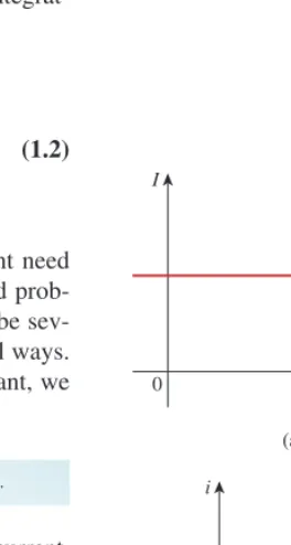
The way we define current as iin Eq. (1.1) suggests that current need not be a constant-valued function. As many of the examples and prob-lems in this chapter and subsequent chapters suggest, there can be sev-eral types of current; that is, charge can vary with time in sevsev-eral ways. If the current does not change with time, but remains constant, we call it a direct current (dc).
A direct current(dc) is a current that remains constant with time.
By convention the symbol Iis used to represent such a constant current. A time-varying current is represented by the symbol i. A common form of time-varying current is the sinusoidal current or alternating current(ac).
An alternating current(ac) is a current that varies sinusoidally with time.
Such current is used in your household to run the air conditioner, refrigerator, washing machine, and other electric appliances. Figure 1.4
Q⫽¢
冮
tt0
idt t0
1 ampere⫽1 coulomb/second
1.3 Charge and Current 7
Andre-Marie Ampere (1775–1836), a French mathematician and physicist, laid the foundation of electrodynamics. He defined the elec-tric current and developed a way to measure it in the 1820s.
Born in Lyons, France, Ampere at age 12 mastered Latin in a few weeks, as he was intensely interested in mathematics and many of the best mathematical works were in Latin. He was a brilliant scientist and a prolific writer. He formulated the laws of electromagnetics. He in-vented the electromagnet and the ammeter. The unit of electric current, the ampere, was named after him.
Historical
I
0 t
(a)
(b)
i
t
0
Figure 1.4
Two common types of current: (a) direct current (dc), (b) alternating current (ac).
8 Chapter 1 Basic Concepts
5 A
(a)
−5 A
(b) Figure 1.5
Conventional current flow: (a) positive current flow, (b) negative current flow.
How much charge is represented by 4,600 electrons?
Solution:
Each electron has C. Hence 4,600 electrons will have
⫺1.602⫻10⫺19 C/electron⫻4,600 electrons⫽ ⫺7.369⫻10⫺16 C ⫺1.602⫻10⫺19
Example 1.1
Practice Problem 1.2
Example 1.2
Calculate the amount of charge represented by six million protons.
Answer:⫹9.612⫻10⫺13C.
Practice Problem 1.1
If in Example 1.2, find the current at s.
Answer:2.707 mA.
t⫽1.0
q⫽(10⫺10e⫺2t) mC,
The total charge entering a terminal is given by mC. Calculate the current at s.
Solution:
At
i⫽5 sin 2p⫹10p cos 2p⫽0⫹10p⫽31.42 mA
t⫽0.5,
i⫽ dq
dt ⫽ d
dt(5t sin 4pt) mC/s⫽(5 sin 4pt⫹20pt cos 4pt) mA t⫽0.5
q⫽5t sin 4pt
shows direct current and alternating current; these are the two most common types of current. We will consider other types later in the book.
Once we define current as the movement of charge, we expect cur-rent to have an associated direction of flow. As mentioned earlier, the direction of current flow is conventionally taken as the direction of pos-itive charge movement. Based on this convention, a current of 5 A may be represented positively or negatively as shown in Fig. 1.5. In other words, a negative current of A flowing in one direction as shown in Fig. 1.5(b) is the same as a current of A flowing in the opposite direction.
1.4 Voltage 9
Example 1.3
Determine the total charge entering a terminal between and s if the current passing the terminal is A.
Solution:
⫽at3⫺ t 2
2b `
2
1
⫽(8⫺2)⫺a1⫺ 1
2b⫽5.5 C
Q⫽
冮
2t⫽1
idt⫽
冮
21
(3t2⫺t)dt
i⫽(3t2⫺t)
t⫽2
t⫽1 s
The current flowing through an element is
Calculate the charge entering the element from to s.
Answer:13.333 C.
t⫽2
t⫽0
i⫽ e4 A, 0 6 t 6 1 4t2 A, t 7 1
a
b v
ab +
−
Figure 1.6 Polarity of voltage v .
ab
Practice Problem 1.3
Voltage
As explained briefly in the previous section, to move the electron in a conductor in a particular direction requires some work or energy trans-fer. This work is performed by an external electromotive force (emf), typically represented by the battery in Fig. 1.3. This emf is also known as voltageor potential difference. The voltage between two points
aand bin an electric circuit is the energy (or work) needed to move a unit charge from ato b; mathematically,
(1.3)
where wis energy in joules (J) and qis charge in coulombs (C). The
voltage or simply v is measured in volts (V), named in honor of
the Italian physicist Alessandro Antonio Volta (1745–1827), who invented the first voltaic battery. From Eq. (1.3), it is evident that
Thus,
Voltage(or potential difference) is the energy required to move a unit
charge through an element, measured in volts (V).
Figure 1.6 shows the voltage across an element (represented by a rectangular block) connected to points aand b. The plus and minus signs are used to define reference direction or voltage polarity. The can be interpreted in two ways: (1) Point ais at a potential of vab vab
(⫺)
(⫹)
1 volt⫽1 joule/coulomb⫽1 newton-meter/coulomb
vab
vab⫽¢ d w
dq
Historical
Alessandro Antonio Volta (1745–1827), an Italian physicist, invented the electric battery—which provided the first continuous flow of electricity—and the capacitor.
Born into a noble family in Como, Italy, Volta was performing electrical experiments at age 18. His invention of the battery in 1796 revolutionized the use of electricity. The publication of his work in 1800 marked the beginning of electric circuit theory. Volta received many honors during his lifetime. The unit of voltage or potential dif-ference, the volt, was named in his honor.
10 Chapter 1 Basic Concepts
9 V
(a)
a
b
+
−
−9 V
(b)
a
b
+
−
Figure 1.7
Two equivalent representations of the same voltage : (a) Point ais 9 V above point b; (b) point bis 9 ⫺ V above point a.
v
ab
Keep in mind that electric current is always throughan element and that electric voltage is always acrossthe element or between two points.
The Burndy Library Collection at The Huntington Library, San Marino, California.
volts higher than point b, or (2) the potential at point awith respect to point bis . It follows logically that in general
(1.4)
For example, in Fig. 1.7, we have two representations of the same volt-age. In Fig. 1.7(a), point ais V above point b; in Fig. 1.7(b), point b
is V above point a. We may say that in Fig. 1.7(a), there is a 9-V
voltage dropfrom ato bor equivalently a 9-Vvoltage risefrom bto
a. In other words, a voltage drop from ato b is equivalent to a volt-age rise from bto a.
Current and voltage are the two basic variables in electric circuits. The common term signalis used for an electric quantity such as a cur-rent or a voltage (or even electromagnetic wave) when it is used for conveying information. Engineers prefer to call such variables signals rather than mathematical functions of time because of their importance in communications and other disciplines. Like electric current, a con-stant voltage is called a dc voltageand is represented by V, whereas a sinusoidally time-varying voltage is called an ac voltageand is repre-sented by v. A dc voltage is commonly produced by a battery; ac
volt-age is produced by an electric generator.
Power and Energy
Although current and voltage are the two basic variables in an electric circuit, they are not sufficient by themselves. For practical purposes, we need to know how much poweran electric device can handle. We all know from experience that a 100-watt bulb gives more light than a 60-watt bulb. We also know that when we pay our bills to the electric utility companies, we are paying for the electric energyconsumed over a certain period of time. Thus, power and energy calculations are important in circuit analysis.
1.5
⫺9⫹9
vab⫽ ⫺vba
1.5 Power and Energy 11
p = +vi
(a)
v
+
−
p = −vi
(b) v + − i i Figure 1.8
Reference polarities for power using the passive sign convention: (a) absorbing power, (b) supplying power.
When the voltage and current directions conform to Fig. 1.8 (b), we have the
ac-tive sign conventionand p⫽⫹vi.
(a) 4 V 3 A (a) + − 3 A 4 V 3 A (b) + − Figure 1.9
Two cases of an element with an absorbing power of 12 W: (a) W, (b) W.p⫽4⫻3⫽12
p⫽4⫻3⫽12
3 A (a) 4 V 3 A (a) + − 3 A 4 V 3 A (b) + − Figure 1.10
Two cases of an element with a supplying power of 12 W: (a)
W, (b) p⫽ ⫺4⫻3⫽ ⫺12W.
⫺12
p⫽ ⫺4⫻3⫽ To relate power and energy to voltage and current, we recall from
physics that:
Poweris the time rate of expending or absorbing energy, measured in
watts (W).
We write this relationship as
(1.5)
where pis power in watts (W), wis energy in joules (J), and tis time
in seconds (s). From Eqs. (1.1), (1.3), and (1.5), it follows that
(1.6)
or
(1.7)
The power pin Eq. (1.7) is a time-varying quantity and is called the
instantaneous power. Thus, the power absorbed or supplied by an ele-ment is the product of the voltage across the eleele-ment and the current through it. If the power has a sign, power is being delivered to or absorbed by the element. If, on the other hand, the power has a sign, power is being supplied by the element. But how do we know when the power has a negative or a positive sign?
Current direction and voltage polarity play a major role in deter-mining the sign of power. It is therefore important that we pay atten-tion to the relaatten-tionship between current i and voltage vin Fig. 1.8(a).
The voltage polarity and current direction must conform with those shown in Fig. 1.8(a) in order for the power to have a positive sign. This is known as the passive sign convention.By the passive sign con-vention, current enters through the positive polarity of the voltage. In this case, or implies that the element is absorbing power. However, if or , as in Fig. 1.8(b), the element is releasing or supplying power.
Passive sign convention is satisfied when the current enters through
the positive terminal of an element and p vi. If the current enters through the negative terminal, p vi.
Unless otherwise stated, we will follow the passive sign conven-tion throughout this text. For example, the element in both circuits of Fig. 1.9 has an absorbing power of W because a positive current enters the positive terminal in both cases. In Fig. 1.10, however, the element is supplying power of W because a positive current enters the negative terminal. Of course, an absorbing power of W is equivalent to a supplying power of W. In general,
⫹Power absorbed⫽ ⫺Power supplied ⫹12 ⫺12 ⫹12 ⫹12 ⫺ ⫽ ⫹ ⫽
vi 6 0
p⫽ ⫺vi vi 7 0
p⫽ ⫹vi
⫺ ⫹
p⫽vi p⫽dw
dt ⫽ dw
dq ⴢ dq
dt ⫽vi
p⫽¢ dw
12 Chapter 1 Basic Concepts
An energy source forces a constant current of 2 A for 10 s to flow through a light bulb. If 2.3 kJ is given off in the form of light and heat energy, calculate the voltage drop across the bulb.
Solution:
The total charge is
The voltage drop is
v⫽ ¢ w
¢q ⫽
2.3⫻103
20 ⫽115 V
¢q⫽i¢t⫽2⫻10⫽20 C
Example 1.4
To move charge q from point a to point b requires J. Find the voltage drop if: (a) C, (b) C.
Answer:(a) ⫺5V, (b) 10 V.
q⫽ ⫺3
q⫽6
vab
⫺30
Practice Problem 1.4
Find the power delivered to an element at ms if the current enter-ing its positive terminal is
and the voltage is: (a) v⫽3i, (b) v⫽3 di兾dt.
i⫽5 cos 60pt A
t⫽3
Example 1.5
In fact, the law of conservation of energy must be obeyed in any electric circuit. For this reason, the algebraic sum of power in a cir-cuit, at any instant of time, must be zero:
(1.8)
This again confirms the fact that the total power supplied to the circuit must balance the total power absorbed.
From Eq. (1.6), the energy absorbed or supplied by an element from time to time t is
(1.9)
Energyis the capacity to do work, measured in joules (J).
The electric power utility companies measure energy in watt-hours (Wh), where
1 Wh⫽3,600 J
w⫽
冮
t
t0
pdt⫽
冮
tt0
vidt
t0
1.5 Power and Energy 13
Solution:
(a) The voltage is hence, the power is
At ms,
(b) We find the voltage and the power as
At ms,
⫽ ⫺14137.167 sin 32.4⬚ cos 32.4⬚ ⫽ ⫺6.396 kW
p⫽ ⫺4500p sin 0.18p cos 0.18p W
t⫽3
p⫽vi⫽ ⫺4500p sin 60pt cos 60pt W v⫽3
di
dt⫽3(⫺60p)5 sin 60pt⫽ ⫺900p sin 60pt V p⫽75 cos2 (60p⫻3⫻10⫺3)⫽75 cos20.18p⫽53.48 W
t⫽3
p⫽vi⫽75 cos2 60pt W v⫽3i⫽15 cos 60pt;
Practice Problem 1.5
Find the power delivered to the element in Example 1.5 at ms if the current remains the same but the voltage is: (a) V,
(b) V.
Answer:(a) 17.27 W, (b) 29.7 W.
v⫽a10⫹5
冮
t
0
idtb
v⫽2i
t⫽5
Example 1.6
How much energy does a 100-W electric bulb consume in two hours?
Solution:
This is the same as
w⫽pt⫽100 W⫻2 h⫽200 Wh
⫽720,000 J⫽720 kJ
w⫽pt⫽100 (W)⫻2 (h)⫻60 (min/h)⫻60 (s/min)
Practice Problem 1.6
A stove element draws 15 A when connected to a 240-V line. How long does it take to consume 180 kJ?
14 Chapter 1 Basic Concepts
Smithsonian Institution.
Historical
1884 Exhibition In the United States, nothing promoted the future of electricity like the 1884 International Electrical Exhibition. Just imagine a world without electricity, a world illuminated by candles and gaslights, a world where the most common transportation was by walk-ing and ridwalk-ing on horseback or by horse-drawn carriage. Into this world an exhibition was created that highlighted Thomas Edison and reflected his highly developed ability to promote his inventions and products. His exhibit featured spectacular lighting displays powered by an impres-sive 100-kW “Jumbo” generator.
Edward Weston’s dynamos and lamps were featured in the United States Electric Lighting Company’s display. Weston’s well known col-lection of scientific instruments was also shown.
1.6 Circuit Elements 15
Figure 1.11
Symbols for independent voltage sources: (a) used for constant or time-varying volt-age, (b) used for constant voltage (dc).
V
(b) +
− v
(a)
+
−
i
Figure 1.12
Symbol for independent current source.
(a) (b)
v +
− i
Figure 1.13
Symbols for: (a) dependent voltage source, (b) dependent current source.
Circuit Elements
As we discussed in Section 1.1, an element is the basic building block of a circuit. An electric circuit is simply an interconnection of the ele-ments. Circuit analysis is the process of determining voltages across (or the currents through) the elements of the circuit.
There are two types of elements found in electric circuits: pas-sive elements and active elements. An active element is capable of generating energy while a passive element is not. Examples of pas-sive elements are resistors, capacitors, and inductors. Typical active elements include generators, batteries, and operational amplifiers. Our aim in this section is to gain familiarity with some important active elements.
The most important active elements are voltage or current sources that generally deliver power to the circuit connected to them. There are two kinds of sources: independent and dependent sources.
An ideal independent source is an active element that provides a
specified voltage or current that is completely independent of other circuit elements.
In other words, an ideal independent voltage source delivers to the circuit whatever current is necessary to maintain its terminal volt-age. Physical sources such as batteries and generators may be regarded as approximations to ideal voltage sources. Figure 1.11 shows the symbols for independent voltage sources. Notice that both symbols in Fig. 1.11(a) and (b) can be used to represent a dc volt-age source, but only the symbol in Fig. 1.11(a) can be used for a time-varying voltage source. Similarly, an ideal independent current source is an active element that provides a specified current com-pletely independent of the voltage across the source. That is, the cur-rent source delivers to the circuit whatever voltage is necessary to maintain the designated current. The symbol for an independent cur-rent source is displayed in Fig. 1.12, where the arrow indicates the direction of current i.
An ideal dependent (or controlled) source is an active element in
which the source quantity is controlled by another voltage or current.
Dependent sources are usually designated by diamond-shaped symbols, as shown in Fig. 1.13. Since the control of the dependent source is achieved by a voltage or current of some other element in the circuit, and the source can be voltage or current, it follows that there are four possible types of dependent sources, namely:
1. A voltage-controlled voltage source (VCVS). 2. A current-controlled voltage source (CCVS). 3. A voltage-controlled current source (VCCS). 4. A current-controlled current source (CCCS).
16 Chapter 1 Basic Concepts
Calculate the power supplied or absorbed by each element in Fig. 1.15.
Solution:
We apply the sign convention for power shown in Figs. 1.8 and 1.9. For , the 5-A current is out of the positive terminal (or into the negative terminal); hence,
For and , the current flows into the positive terminal of the ele-ment in each case.
For , we should note that the voltage is 8 V (positive at the top), the same as the voltage for since both the passive element and the dependent source are connected to the same terminals. (Remember that voltage is always measured across an element in a circuit.) Since the current flows out of the positive terminal,
We should observe that the 20-V independent voltage source and dependent current source are supplying power to the rest of the network, while the two passive elements are absorbing power. Also,
In agreement with Eq. (1.8), the total power supplied equals the total power absorbed.
p1⫹p2⫹p3⫹p4⫽ ⫺100⫹60⫹48⫺8⫽0
0.2I
p4⫽8(⫺0.2I)⫽8(⫺0.2⫻5)⫽ ⫺8 W Supplied power
p3,
p4
p3⫽8(6)⫽48 W Absorbed power
p2⫽12(5)⫽60 W Absorbed power
p3
p2
p1⫽20(⫺5)⫽ ⫺100 W Supplied power
p1
Example 1.7
p2
p3 I = 5 A
20 V
6 A
8 V 0.2I
12 V
+
−
+
−
+ −
p1 p4
Figure 1.15 For Example 1.7.
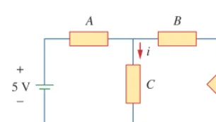
i
A B
C 10i
5 V +−
+
−
Figure 1.14
The source on the right-hand side is a current-controlled voltage source.
Dependent sources are useful in modeling elements such as transis-tors, operational amplifiers, and integrated circuits. An example of a current-controlled voltage source is shown on the right-hand side of Fig. 1.14, where the voltage of the voltage source depends on the current i through element C. Students might be surprised that the value of the dependent voltage source is V (and not A) because it is a voltage source. The key idea to keep