SELF-LOCALIZATION OF A MULTI-FISHEYE CAMERA BASED AUGMENTED
REALITY SYSTEM IN TEXTURELESS 3D BUILDING MODELS
S. Urban, J. Leitloff, S. Wursthorn and S. Hinz
Institute of Photogrammetry and Remote Sensing (IPF), Karlsruhe Institute of Technology (KIT) Englerstr. 7, D-76137 Karlsruhe, Germany
(steffen.urban, jens.leitloff, sven.wursthorn, stefan.hinz)@kit.edu http://www.ipf.kit.edu
Commission III WG III/3
KEY WORDS:computer vision, fisheye camera, real-time object detection, model-based tracking, augmented reality
ABSTRACT:
Georeferenced images help planners to compare and document the progress of underground construction sites. As underground posi-tioning can not rely on GPS/GNSS, we introduce a solely vision based localization method, that makes use of a textureless 3D CAD model of the construction site. In our analysis-by-synthesis approach, depth and normal fisheye images are rendered from presampled positions and gradient orientations are extracted to build a high dimensional synthetic feature space. Acquired camera images are then matched to those features by using a robust distance metric and fast nearest neighbor search. In this manner, initial poses can be obtained on a laptop in real-time using concurrent processing and the graphics processing unit.
1 INTRODUCTION
This paper describes a multi fisheye camera system to support localization of a mobile augmented reality (AR) client on sub-way construction sites. It is part of the work of a joint research group on computer-aided collaborative subway track planning in multi-scale 3D city and building models. It addresses the chal-lenges of integrating the collaborative planning effort within a synchronous software workflow for seamlessly modeling, man-aging and analyzing both CAD and GIS based 3D models (Bre-unig et al., 2011). A mobile client is supposed to support the planning process by augmenting camera images with 3D models of distinct construction stages on-site. Consequently, the camera snapshots need to be localized and orientated within the spatial context of the 3D model. The overlay of projected 3D data on these camera snapshots is supposed to help planers to compare planning stages with the actual status (Breunig et al., 2012).
The interior orientation of three cameras with fixed focus fisheye lenses is determined in a calibration step and is considered con-stant for all images grabbed with a particular camera. The six degrees of freedom of the exterior camera orientation need to be determined with every new image. A major challenge is the lack of GNSS signals at subway construction sites, which would ease getting at least an initial position and some stabilization points that are needed for a continuous tracking. The process of deter-mining the six degrees of freedom of the camera’s exterior ori-entation within the given 3D model with feature correspondences extracted both from the images and the untextured 3D models alone is the purpose of our sub-project within the research group.
We do not use depth images from stereo or range imaging de-vices due to their limited range and field of view (Weinmann et al., 2011). Cameras do easily fit on a building-site helmet in con-trast to e.q. laser scanning devices. In this paper we will concen-trate on the initialization step of our designated tracking process. We use gradient orientations, extracted from rendered images of the 3D model and compare these to gradient orientations in the real camera images by using a robust distance metric, to find the camera pose in the model.
1.1 Previous Research
The fact, that only an unknown fraction of the building model will be visible on the camera images is challenging and has rarely been addressed in other publications on model based tracking. In (David et al., 2003, David et al., 2004, Wuest et al., 2005) edge based methods compare 3D model edges projected into the im-age with regions that have high imim-age gradients. (Drummond and Cipolla, 2002) project 3D points that lie on model edges onto the image plane and minimize distances to the nearest edges in the image. The matched 3D-2D point correspondences are used to solve the registration of the image within the 3D model. The sys-tem is supposed to operate in real-time, but a good initial registra-tion is needed in order to minimize the distances. (Behringer et al., 2002), (Reitmayr and Drummond, 2006) and (Simon, 2011) need additional sensors for position (GPS) and orientation to ini-tialize their tracking systems in large outdoor environments. (Wuest et al., 2007) propose the use of an inertial measurement unit in the future for initialization.
(Ulrich et al., 2009) use offline training of various possible ob-ject poses to achieve an image based initialization. (Ottlik and Nagel, 2007) show automatic initialization in the domain of ve-hicle tracking in traffic videos. Both implementations are robust against occlusions but the models are supposed to completely fit into the images.
In the remainder of this paper the multi fisheye camera system is introduced first as well as the calibration of the camera and the system. Afterwards the self-localization method is shown and each step in the process is detailed. Subsequently a test on sim-ulated data is carried out, to adjust parameters that are crucial to the initialization and to evaluate pose estimates. Finally we give a conclusion and describe our future work.
2 CAMERA SYSTEM
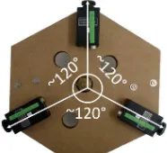
Fisheye cameras are often superior to narrow angle perspective cameras in tracking tasks (Svoboda, 1998, Micuˇsık and Pajdla, 2006). Features stay longer in the field-of-view during camera movement, partially occluded model parts occur only in small image regions and pose estimation is often better conditioned. To further improve the quality, stabilize the pose estimation and pro-vide a maximum number of visible features, three fisheye cam-eras are used. The horizontal angle between each principal axis averages120◦, creating a360◦panoramic view of the environ-ment. This particular camera arrangement was chosen to allow a robust localization even if one or two cameras fail to maintain their pose estimate, which could happen on construction sites. (Fig. 1).
Figure 1: System configuration of the three fisheye cameras.
2.1 Fisheye Camera Model and Calibration
Camera calibration is essential to many vision tasks. The result is a mapping function that describes the relation between a pixel on the image plane to its corresponding 3D ray. In an analysis-by-synthesis tracking approach, the calibration is crucial to the rendering step, as the virtual camera needs to fulfill the same mapping functions as the real camera. The calibration of a fish-eye camera differs from perspective camera calibration, because camera models need to allow for incident angles greater90◦. In recent years, different models and calibration methods for fish-eye cameras have been published (Scaramuzza et al., 2006, Mei and Rives, 2007, Micuˇsık, 2004). A comprehensive overview is given in (Puig et al., 2012). We chose the unified taylor model in-troduced by (Scaramuzza et al., 2006). The following section de-tails parts of the model that are important for the rendering (Sec. 3.2). LetP= (X, Y, Z)Tbe a point in world coordinates. Then the functionf(u, v), that maps the 2D image pointp= (u, v)T toP, i.e. the forward-projection, is calibrated:
P =
The fisheye lens is assumed to be rotational symmetric thus the polynomial can be written as:
f(ρ) =a0+a2ρ2+...+anρn (2)
with
ρ= √u2+v2 (3)
We chose a polynomial degree ofn = 4in this paper, which gave the best calibration results. During rendering, the mapping function of a 3D object point onto the image plane is needed. This back-projection is modeled by the inverse off(ρ):
d=f−1(Θ) (4)
where d is the distance of a back projected point from the image center and
Θ = arctan Z2
X2+Y2
(5)
is the incident angle to the principal axis. Thus temporary image coordinates can be calculated:
Then a affine mapping is applied to compensate for small dis-tortions, non-square pixels and misalignments between lens and image plane axis. Finally the image coordinates are related to the upper left image corner by adding the coordinates of the principal point:
After determination of each cameras intrinsic parameters, the mul-tiple fisheye camera configuration can be examined. In order to fully exploit the configuration, relative poses between each cam-era are necessary. In this way, the systems exterior orientation can be maintained, even if two cameras fail to estimate their pose. As each camera points in a different direction, a calibra-tion object that is only visible in one camera at a time, like a cal-ibration pattern, is unusable. Hence we directly made use of the 3D building model in which the system is moving (for a descrip-tion of the model see secdescrip-tion 4). A trajectory was recorded and synchronous keyframes from this trajectory were selected. Then 2D image features and their corresponding 3D coordinates in the model were manually extracted. Next, the exterior orientation for each keyframe and each camera was estimated from these 2D-3D correspondences. The relative poses were then extracted from a series of exterior orientations for each camera.
3 SELF-LOCALIZATION
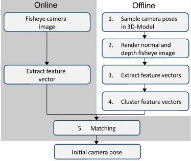
The system is supposed to estimate its initial position without hu-man intervention. This process is detailed in Figure 2. It can be divided into two parts, i.e. online and offline phase. During theofflinephase, the system creates virtual camera poses, renders synthetic views of the model and extracts features from them. These features are then clustered and saved. In theonlinephase the cameras acquire images and extract feature vectors from them likewise. These features are then matched to the synthetic fea-tures for each frame and each camera with a particular metric. If the metric exceeds a certain threshold the virtual camera pose is assigned to the real camera and the system has localized itself in the model. The following sections detail each consecutive step shown in Figure 2.
3.1 Position Sampling
At first glance the camera pose in the 3D model seems to be en-tirely random. This would require a huge amount of pre-sampled positions and hence to many feature vectors to process. But since the system is supposed to be head mounted, some constraints can be applied.
Figure 2: Flow-chart of the self-localization process.
and the view direction is expressed by a polar (or yaw) angleφ
and a azimuth (or pitch) angleθ. Now assumptions about the range of values can be made. For instance, the operator tilts his head in a narrow range which constrains the pitch angleθ. In this workθis set to[−20◦,20◦]from the horizon and is sampled in 10◦steps. The yaw angle is free from[0,360◦]and is sampled in 10◦steps in this example. The horizontal sampling is a parameter that can be optimized, though, because of the similarity of adja-cent views (Fig. 3). Further the operators body height is known
(a) view onto x-y plane (b) view onto y-z plane
Figure 3: (a) Camera view directions in the x-y plane. Depicted is the sampling of the polar angle. (b) Camera view directions in the y-z plane. Depicted is the sampling of the azimuth angle. This covers approx. the range an operator would tilt his head.
and thus theZcomponent can be set accordingly. This still leaves theX andY component free. To further reduce the number of presampled positions,XandY are sampled in a rectangular grid at levelZ(Fig. 4). The spacing between each position determines the density of the position sampling. We chose a grid density of 0.5 m for this work. Sampling the view sphere also prevents from presampling positions for each camera separately since the dis-tance from each camera to the origin is small w.r.t the density of the grid.
3.2 Rendering
After sampling virtual camera poses in the 3D model, synthetic views of the 3D model are generated (Fig. 5). This approach is called analysis-by-synthesis (Wuest et al., 2007). The idea is, to render a view of the 3D model, extract all visible edges from it and match them to the real camera image of the model. OpenGL (Khronos Group, 2013) is used to perform hidden line removal and to render the image in a normal and a depth image. This two-time rendering is necessary, as the normal image contains all crease edges and the depth image all step edges. A conventional rendering pipeline only supports two kinds of projection matri-ces, either orthographic or perspective. Neither applies to fisheye cameras.
Figure 4: Distribution of view speres in the horizontal grid. The z-coordinate of the grid resamples approx. the height of the op-erators head.
Thus we elude the fixed vertex processing by using a custom ver-tex shader. Latter allows us to manipulate the geometry of the scene. First, the model is transformed to the camera reference frame using the model-view matrix, which contains the camera pose in the 3D model. Now the incident angleΘfor each vertex can be calculated Eq. (5) and the inverse mapping Eq. (4) for each viewing ray is determined. Then the corresponding pixel is calculated according to Eq. (6), Eq. (7). Hereby the calibrated mapping function of each real camera is exploited in a vertex shader, to extend the simple perspective camera view to a geo-metrically correct fisheye view.
After vertex processing, a fragment shader is used to color the pixels according to their normal (Fig. 5(a)) and depth (Fig. 5(b)) information respectively. At this point it is important to note, that the normal and depth values are independent of the vertex transformation. The z-value of each vertex is untouched during the mapping as well as the normal vectors. Latter are assigned to each face and vertex respectively and are calculated prior to the mapping. Otherwise the fisheye mapping would change these information and the resulting image would contain wrong normal and depth values.
(a) normal image (b) depth image Figure 5: Rendered fisheye images for combined crease edge (a) and step edge (b) extraction.
Image pyramids help to speed up feature extraction, but the pro-cess of generating these pyramids for both images, i.e. normal and depth images, slows down the overall process. Thus, in-stead of rendering a full resolution image followed by subsequent downsampling, we chose to render different image octaves di-rectly by applying different viewport sizes, followed by concur-rent edge extraction.
3.3 Feature Extraction
smoothing step can be omitted since rendered images do usu-ally not contain noise. Then a gradient magnitude imageIC =
q
G2
C,y+G2C,xis calculated for each channel, whereGC,xand
GC,yare the sobel derivatives inxandydirection for a channel
C ∈ {R, G, B, D}, where the first three belong to the normal and the last to the depth image.
All magnitude arising from the normal image are tested against a threshold. Latter corresponds to a orientation change. Round structures and surfaces in 3D models are appoximated by many faces. The edge extraction would yield all edges, even if they are not present in the real image. To avoid this, the threshold has to be set accordingly. If no edge has been detected for a particular pixel in the normal image, the depth image is tested. In this case another threshold needs to be set, which corresponds to the z-buffer range and precision. We then choose the highest magnitudeGˆof all magnitude images for a particular pixelu, v
and extract its orientation
Φ(u, v) = arctan GˆC,y(u, v) ˆ
GC,x(u, v)
!
(8)
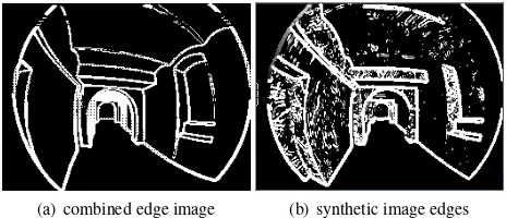
The combined gradient image is depicted in Figure 6(a). Edges are not thinned using non maximum suppression. However it showed, that broader edges lead to better matching results, as there will never be a perfect match and thus broader edges serve indirectly as a pull-in range for the nearest neighbor matching.
(a) combined edge image (b) synthetic image edges Figure 6: (a) Combined edge image. After extracting edges from normal and a depth image seperately, the maximum gradient is chosen to extract edge orientations. (b) Extracted edges from ren-dered model. The added noise to pose and image, respectively is visible.
Each combined edge image is then reshaped to a 1D holistic fea-ture vector that contains the orientations of all visible edges. In our implementation the feature extraction is carried out on the 4th pyramid level. Here the images size is 49×65 pixels leading to a feature dimension of 3185.
3.4 Feature Matching
The last step to self-localization is crucial. The offline created, synthetic feature vectors have to be matched against the incom-ing camera images, usincom-ing a robust distance metric. Since a lin-ear slin-earch trough all features for an exact match would not be real-time capable, an efficient way of clustering and searching a nearest neighbor to a given feature vector is used.
3.4.1 Distance Metric The matching is solely performed on edges. Hence the distance metric has to be robust to occlusion, illumination change and clutter. Geometric deformations can be neglected since we use a rigid 3D model. We use the metric de-fined in (Hinterstoisser et al., 2012) which is adapted from (Ste-ger, 2002). Latter shows its robustness to occlusions and illumi-nation changes by taking the absolute value of the cosine: Unsim-ilar egdes contribute little to the sum and negative values, caused
by different illuminations, are mapped to the positive range. The metric is based on gradient orientations to determine a measure of similarity. In contrast to (Steger, 2002), Eq. (9) minimizes the number of features and calculations during tree construction and matching:
d = w·h
X
i=1
|cos (Φsi−Φti)| (9)
whereΦsiandΦri are gradient orientations of search and
tem-plate image andw,hare width and height of the search image.
3.4.2 Clustering and Nearest Neighbor Search As presented in Section 3.1 a lot of virtual cameras are sampled and high di-mensional feature vectors are extracted. For instance, 50 presam-pled positions with an angular increment of10◦lead to 9000 fea-ture vectors. Taking the feafea-ture dimension of 3185 from the last section, this would require∼30 million calculations in a linear search, as Eq. (9) had to be computed for each template image against the search image.
Hence, we experimented with multiple randomized kd-trees and hierarchical trees with k-means clustering and use the implemen-tation of flann (Muja and Lowe, 2009) a library for fast approx-imate nearest neighbor search to high-dimensional feature vec-tors. Usually the performance of nearest neighbor search de-creases with the dimensionality of the feature vector. But (Muja and Lowe, 2009) show that for real world data sets, where strong correlation between dimensions exist, the precision remains al-most constant. Both trees have different parameters which are crucial relating to speed and precision. The next section details the algorithm choice.
4 RESULTS AND DISCUSSION
For all our experiments, a L-shaped part of the buildings base-ment is used, which is characterized by bad light conditions, par-tially narrow walls and objects occluding edges. The 3D model is the result of a laser scan point cloud. The point cloud was simplified, cleaned and meshed. The final model has∼550.000 vertices and∼190.000faces and consists of flat and round sur-faces.
4.1 Simulated Data
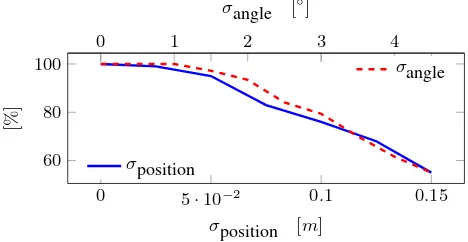
To test our method and adjust parameters, i.e. the number of presampled positions, sampling density, edge thresholds, speed and search parameters the 3D model was rendered from 100 per-turbed poses. These poses are randomly drawn from the set of all 9000 presampled poses. To simulate false and missing edges and to add image noise that occurs in a real world scenario, we attach a noisy, coarse resolution wall texture to the model and render it. The edges of the resulting image are depicted in Figure 6(b).
0 5·10−2 0.1 0.15 60
80 100
0 1 2 3 4
σposition [m]
[%]
σangle [◦]
σposition
σangle
Figure 7: Precision of matching with increasing noise.
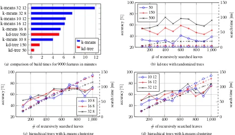
search speed is crucial. The linear search for 9000 features takes about 370ms on a Intel i7-3630QM CPU, which is not sufficient for real-time applications. Hence different trees and parameter combinations for flann (Muja and Lowe, 2009) were tested, to evaluate the accuracy against the linear search.
Again 100 textured images are rendered from perturbed positions. Then the 9 different trees from Figure 8(a) are searched. This time however, the number of recursively searched leaves is in-creased. This leads to a better search precision on the one hand, but reduces the search speed on the other. Thus, a trade-off be-tween search speed, precision and tree build time has to be found. Figure 8 shows search speed and corresponding precision for an increasing search depth. For all six hierarchical k-means trees the search time increases faster than the precision. Consider-ing that for real-time AR-applications all calculations for each camera have to be finished within 45ms≈22fps (fisheye camera fps), the k-means tree is only feasible for lower search depths. However at a search depth of 300, the precision hardly exceeds 50%. A higher number of iterations during build time resulted in a longer build time but did not significantly improve the preci-sion.
Hence we chose the randomized kd-tree. Even for 500 trees the build time is feasible and the precision for the simulated scenario keeps up with the hierachical k-means trees. The huge advantage is the search speed which is feasible for real-time AR.
4.2 Real Data
After adjusting parameters during the simulation, we tested our system under real conditions. To exploit the full spherical view of the scene, we create panoramic feature vectors, i.e. we stack the feature vectors of all three cameras together. We then match those to prerendered panoramic features from the feature creation step. The position sampling scheme is basically the same, but instead of rendering one image per sample position, we render three images, using the known relative poses of the cameras.
Since we did not yet acquire ground truth for each frame of an entire full frame rate trajectory, we conducted a qualitative visual verification of the initialization results for the 14 keyframes from Section 2.2 where the exterior orientation of the system was de-termined with a total station. We found that the initialization was correct in 11 out of the 14 keyframes. Figure 9 depicts such a case (and comprises a link to the sequence). The correctly matched model edges are overlaid in green. Note that the model edges do not fit perfectly. On the one hand we initialized the system from discrete poses, but in reality the trajectory is continuous, i.e. we initialized the nearest neighbor of the true pose. On the other hand the initialization is carried out on the lowest scale level. From here on, the pose has to be refined by, e.g. minimizing the squared distances to the nearest edge on each scale level.
5 CONCLUSIONS AND FUTURE WORK
In this paper, a novel approach to image based self-localization of a multi fisheye camera system in texture-less 3D models was pre-sented. To approach the problem of a comparatively big model and the fact, that the camera pose is inside the model and only parts of it are visible at a current pose, virtual camera poses are presampled and fisheye camera views are rendered using OpenGL and a custom vertex shader. Then feature vectors based on gra-dient orientations are extracted on low pyramid levels and clus-tered for fast nearest neighbor search. A robust distance metric was used to match features during nearest neighbor search, which handles occlusions, clutter, illumination and contrast changes.
To further increase search precision and search speed for future work, redundancies between feature vectors have to be elimi-nated, i.e. two adjacent camera poses that contain approximately the same information can be omitted. In addition, all feature vec-tors live in memory during runtime and a decrease to the essen-tial number could increase the scalability, however the presented configuration allocates 110MB (9000×3185×4byte) memory which is viable even for larger feature sets.
One drawback of the method presented is, that it depends on a threshold to declare an initialization correct. The nearest neigh-bor search gives the best (highest distance metric sum) result for a given frame, which is not instantaneously correct and there might be other neighbors that are almost equally good and thus could be probably correct. Thus, in future work, we will base our method on a particle filter. Each presampled positions can be seen of as a particle and the distance metric can be used as a likelihood mea-sure for each consecutive frame. This means, that all particles will have a high likelihood in the neighborhood of the correct pose, which can be described by a probability density function over the state space (presampled poses).
REFERENCES
Behringer, R., Park, J. and Sundareswaran, V., 2002. Model-based vi-sual tracking for outdoor augmented reality applications. In: Interna-tional Symposium on Mixed and Augmented Reality (ISMAR), Darm-stadt, pp. 277–278.
Breunig, M., Borrmann, A., Rank, E., Schilcher, M. and Hinz, S., 2012. Towards 3d geoinformatics and computational civil engineering support for cooperative tracks planning. In: Proceedings of FIG Working Week, Rome.
Breunig, M., Rank, E., Schilcher, M., Borrmann, A., Hinz, S., Mundani, R., Ji, Y., Menninghaus, M., Donaubauer, A., Steuer, H. et al., 2011. Towards computer-aided collaborative subway track planning in multi-scale 3d city and building models. In: Proceedings of the 6th 3D geoinfo conference, Vol. 17.
David, P., Dementhon, D., Duraiswami, R. and Samet, H., 2003. Simul-taneous pose and correspondence determination using line features. In: IEEE Conference on Computer Vision and Pattern Recognition, Madison, USA, pp. 424–431.
David, P., Dementhon, D., Duraiswami, R. and Samet, H., 2004. Soft-posit: Simultaneous pose and correspondence determination. Interna-tional Journal of Computer Vision 59(3), pp. 259–284.
Drummond, T. and Cipolla, R., 2002. Real-time visual tracking of com-plex structures. IEEE Transaction on Pattern Recognition and Machine Intelligence 24(7), pp. 932–946.
Hinterstoisser, S., Cagniart, C., Ilic, S., Sturm, P., Navab, N., Fua, P. and Lepetit, V., 2012. Gradient response maps for real-time detection of textureless objects. Pattern Analysis and Machine Intelligence, IEEE Transactions on 34(5), pp. 876–888.
0 2 4 6 8 10 12
(a) comparison of build times for 9000 features in minutes
200 400 600 800 1,000
#of recursively searched leaves
accurac
(b) kd-tree with randomized trees
200 400 600 800 1,000
#of recursively searched leaves
accurac
(c) hierachical trees with k-means clustering
200 400 600 800 1,000
#of recursively searched leaves
accurac
(d) hierachical trees with k-means clustering
Figure 8: Search precision vs. speed (dashed lines) for 9 different trees (number of features for all plots: 9000). Angle noise was set toσangle= 1.5◦, position noise toσ
pos= 0.05m. The accuracy is related to the precision at this particular noise level for the linear search. Parameters: k-meansbranching factorandnumber of iterations, kd-treenumber of trees.
Figure 9: All three fisheye images overlaid with model edges after correct self-localization with the real image sequence. Complete sequence seehttp://www2.ipf.kit.edu/Projekte/3DTracks/.
Micuˇsık, B., 2004. Two-view geometry of omnidirectional cameras. PhD thesis, Czech Technical University.
Micuˇsık, B. and Pajdla, T., 2006. Structure from motion with wide cir-cular field of view cameras. Pattern Analysis and Machine Intelligence, IEEE Transactions on 28(7), pp. 1135–1149.
Muja, M. and Lowe, D. G., 2009. Fast approximate nearest neighbors with automatic algorithm configuration. In: International Conference on Computer Vision Theory and Application (VISSAPP’09), INSTICC Press, pp. 331–340.
Ottlik, A. and Nagel, H.-H., 2007. Initialization of model-based vehi-cle tracking in video sequences of inner-city intersections. International Journal of Computer Vision 80(2), pp. 211–225.
Puig, L., Berm´udez, J., Sturm, P. and Guerrero, J., 2012. Calibration of omnidirectional cameras in practice: A comparison of methods. Com-puter Vision and Image Understanding 116(1), pp. 120 – 137.
Reitmayr, G. and Drummond, T., 2006. Going out: Robust model-based tracking for outdoor augmented reality. In: Proceedings of the Interna-tional Symposium on Mixed and Augmented Reality (ISMAR). Scaramuzza, D., Martinelli, A. and Siegwart, R., 2006. A flexible tech-nique for accurate omnidirectional camera calibration and structure from motion. In: Computer Vision Systems, 2006 ICVS’06. IEEE Interna-tional Conference on, IEEE, pp. 45–45.
Simon, G., 2011. Tracking-by-synthesis using point features and pyra-midal blurring. In: International Symposium on Mixed and Augmented Reality (ISMAR), pp. 85–92.
Steger, C., 2002. Occlusion, clutter, and illumination invariant object recognition. International Archives of Photogrammetry Remote Sensing and Spatial Information Sciences 34(3/A), pp. 345–350.
Svoboda, T., 1998. Motion estimation using central panoramic cameras. Ulrich, M., Wiedemann, C. and Steger, C., 2009. Cad-based recognition of 3d objects in monocular images. In: IEEE International Conference on Robotics and Automation, Kobe, Japan, pp. 1191–1198.
Weinmann, M., Wursthorn, S. and Jutzi, B., 2011. Semi-automatic image-based co-registration of range imaging data with different characteris-tics. In: PIA11 - Photogrammetric Image Analysis, Vol. 38 Part 3/W22, pp. 119–124.