Algorithmica
©1998 Springer-Verlag New York Inc.
On-Line Load Balancing and Network Flow
1S. Phillips2and J. Westbrook3
Abstract. In this paper we study two problems that can be viewed as on-line games on a dynamic bipartite graph. The first problem is on-line load balancing with preemption. A centralized scheduler must assign tasks to servers, processing on-line a sequence of task arrivals and departures. Each task is restricted to run on some subset of the servers. The scheduler attempts to keep the load well-balanced. If preemptive reassignments are disallowed, Azar et al. [3] proved a lower bound ofÄ(√n)on the ratio between the maximum load achieved by an on-line algorithm and the optimum off-line maximum load. We show that this ratio can be greatly reduced by an efficient scheduler using only a small amount of rescheduling.
We then apply these ideas to network flow. Cheriyan and Hagerup [6] introduced an on-line game on a bipartite graph as a fundamental step in improving algorithms for computing the maximum flow in networks. They described a randomized strategy to play the game. King et al. [11] studied a modified version of this game, called “node kill,” and gave a deterministic strategy. We obtain an improved deterministic algorithm for the node kill game (and hence for maximum flow) in all but the sparsest graphs. The running time achieved is
O(mn logm/nn+n2log2+εn), compared with King et al.’s O(mn+n2+ε).
These problems combine a demand for good competitive ratios with more traditional requirements of implementation efficiency. Our solutions deal with the tradeoffs between these measures.
Key Words. Network flow, Optimization, On-line algorithm, Competitive analysis, Load balancing, Pre-emption, Scheduling.
1. Introduction
1.1. Load Balancing with Preemption. In the dynamic load balancing problem we have a fixed set V of n servers and a dynamic set of tasks U that arrive and depart on-line. Each task has edges to a subset S of the servers and at all times it must be matched to some server in S. A server may have multiple tasks assigned to it simultaneously. The
load on a server is the number of tasks currently assigned to it.
Azar et al. [3] proposed the dynamic load balancing problem as an abstraction of scheduling problems that can occur in heterogenous networks containing workstations, I/O devices, etc. Servers correspond to communication channels and tasks to requests for communication links between devices. A network controller must coordinate the channels so that no channel is too heavily loaded. The request sequence is unknown in advance.
Let Load(A, σ ) be the maximum load on any server after scheduler A processes sequenceσ. Following the conventions of competitive analysis, we say the competitive
1The research by S. Phillips was partially supported by NSF Grant CCR-9010517 and grants from Mitsubishi and OTL. The research by J. Westbrook was partially done while he was visiting DEC Systems Research Center, and was partially supported by NSF Grant 9009753.
ratio of A is the supremum over sequencesσ of Load(A, σ )/Load(OPT, σ ), where
Load(OPT, σ )is the minimum possible maximum load afterσ.
Azar et al. [4] studied dynamic load balancing under two restrictions: first, that no tasks ever depart; and second, that tasks cannot be preempted. Azar et al. showed that the greedy strategy has a competitive ratio of log n and that this is optimal within constant factors among both deterministic and randomized algorithms. If for each task the eligible subset is all servers, however, then the competitive ratio falls to 2−εfor some small constantε[10], [5].
Azar et al. [3] studied the dynamic load balancing problem when tasks both arrive and depart, but retained the restriction that tasks cannot be preempted. In this version the picture is worse: using our definition of Load(A, σ ), the best possible competitive ratio is n. Azar et al. defined Load(A, σ )to be the maximum load at any time during σ and showed under this definition that the greedy strategy has a ratio of 2(n2/3). They also proved a bound of Ä(√n)on the competitive ratio of any randomized or deterministic strategy. (Again, under this definition the ratio is 2−εif the eligible subset is all servers.) In both [3] and [4] the same bounds are shown for an extension where tasks have weights. These strong bounds indicate that the performance of an on-line scheduler may be severely impacted by the lack of information about future tasks. The
O(√n)lower bound has recently been shown to be tight [2].
We address the problem of the huge lower bound on the achievable competitive ratio by giving the scheduler a little more power. We study load balancing with task
preemption. That is, the scheduler is allowed to reassign tasks to servers as new jobs
arrive, in order to keep the load well-balanced. In this problem we cannot simply measure an on-line algorithm by a competitive ratio. Since the scheduler is free at any point to reassign all tasks, it can always guarantee a competitive ratio of 1. On the other hand, this approach may be undesirable in practice. Preempting a task can be an expensive process and one may be willing to accept an imbalance in the load in order to avoid the expense of reassignments. Similarly, one may wish to limit the time the scheduler spends processing task arrivals and departures, in which case computing an optimal assignment may be too expensive.
With this in mind, we measure the quality of an on-line scheduler for preemptive load balancing in three ways: the competitive ratio it achieves; the number of preemptive
reassignments performed during a run; and the overall computation time during a run.
In Section 2 we show that the competitive ratio can be greatly reduced by a small amount of preemptive rescheduling. We consider two algorithms, A and Balance-B. The Balance-A algorithm keeps the maximum on-line load within 12(log n)/ρtimes the optimum maximum load while performingρm preemptive reassignments on a
se-quence of m task arrivals and departures. Here n is the number of servers, m is the total number of tasks, andρis an arbitrary parameter less than 1 that may be a function of n or m. Balance-B is a version of Balance-A that incurs a small increase in the maximum load to keep computation costs low (linear in the total degree of the arriving tasks plus logarithmic overhead per task arrival or departure).
be computed in2(n3log n)time using binary search and a b-matching algorithm [12]. This results in a ratio of 1,2(m2)reassignments, and2(mn3log n)total computation. Our algorithms extend to more general versions of the problem where both tasks and servers may arrive and depart, and where tasks have an associated weight and the maximum weighted load must be minimized.
1.2. Network Flow. The node kill game, introduced by King et al. [11], is played on a bipartite graph G =(U,V,E)where|U| = |V| =n and|E| =m. We refer to the
nodes in U as items and the nodes in V as columns. The rules of the game are as follows:
1. At the start of each turn, player A (the algorithm) must designate a current edge{u, v} for each item u. We say u is assigned tov.
2. Player B (the adversary) begins a turn by either removing a single edge (an edge kill) or removing all edges incident to a single column (a node kill). If an item u has no remaining edges it is out of the game.
3. Player A completes the turn by designating a new current edge for any each item u whose former current edge was removed. In addition, player A may redesignate the current edge of any other item y.
4. Player B scores one point for each current edge it removes in a node kill. It scores zero points for each edge removed by an edge kill. It scores one point each time player A redesignates the current edge of an item.
The similarity to the on-line load balancing problem is evident. Clearly, player A should keep the columns balanced in some way, to prevent player B from gaining too many points during node kills. Edge kills are closely related to task departures.
The number of points scored by B is the number of dynamic tree operations performed by the Goldberg–Tarjan algorithm for maximum flow [9]. The correspondence between the game and the running time for network flow is given by the following theorems from [11].
THEOREM1. Given a strategy to play the node kill game, scoring at most P(n,m)
points with an implementation cost of C(n,m), maximum flow in a graph with N nodes
and M edges can be computed in time C(N2,NM)+O(N3/2M1/2+P(N2,NM)log N).
THEOREM2. When the node kill game is used for network flows, if at most P(n,m)
points are scored in the node kill game, then the number of edge kills is at most O(√nm+ P(n,m)).
Cheriyan and Hagerup [6], [7] first introduced a restricted form of this game, in which player A may not redesignate edges, and described a randomized strategy. Alon [1] derandomized this strategy. King et al. extended the game to the form described above and found an improved deterministic strategy.
We apply ideas from on-line load balancing to play the node-kill game well. The
ratio algorithm for the node kill game is presented in Section 3. It provides a speedup
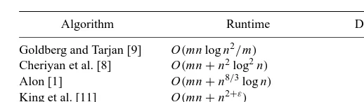
Table 1. Running time for network flow.
Algorithm Runtime Deterministic?
Goldberg and Tarjan [9] O(mn log n2/m) Yes Cheriyan et al. [8] O(mn+n2log2n) No
Alon [1] O(mn+n8/3log n) Yes
King et al. [11] O(mn+n2+ε) Yes
This paper O(mn logm/nn+n2log2+εn) Yes
In addition to the running time of a maximum flow algorithm, Cheriyan et al. studied the number of real number operations, referred to as flow operations. Their randomized algorithm gives the first bound of o(nm)on the number of flow operations—in particular, an expected bound of O(n3/2m1/2log n+n2(log n)2/log(2+n(log n)2/m)). King et al. have shown that their extended deterministic algorithm performs only O(m1/2+εn3/2−ε·
log1m/n/2 n log n)flow operations.4We show that our algorithm also achieves this number of flow operations.
2. Dynamic Load Balancing with Preemption. Our algorithms combine the greedy
strategy of assigning an arriving task to an adjacent server of minimum load with an efficient rebalancing technique that occasionally redistributes the work of heavily loaded servers.
2.1. Balance-A. This section describes a simple and efficient algorithm, Balance-A. There is much flexibility in the details of the algorithm and its implementation, and its robustness and simplicity indicate that it may be useful in other scheduling and load balancing applications.
The algorithm takes a parameterρwhich is the desired ratio of preemptive reassign-ments to tasks leaving the system. We constrain 1≥ρ >0. For the moment we assume thatρ is a fixed constant, although the algorithm will work withρ a function of n or even s, where s is the number of tasks currently in the system.
A greedy assignment of a task means that the task is assigned to the adjacent server of minimum load. Balance-A works as follows. When a new task u arrives, it is assigned greedily to some serverv. After each task arrival or departure, Balance-A executes a load balancing procedure described below. The procedure first makes an estimate of the optimum maximum load. It then performs a limited number of reassignments designed to bring the loads into approximate balance, based on that estimate.
If we order the tasks on a server by the time they were last assigned there then we can think of each server supporting a column of tasks, with the earliest assigned tasks at the bottom and the latest assigned on top. The height of task u, h(u), is the number of tasks currently below it. The height of serverv, h(v), is the load onv. We define a third quantity,
m(v), which roughly corresponds to the maximum heightvever had. When task u is
assigned to serverv, set h(u)=h(v), h(v)=h(v)+1, and m(v)=max{m(v),h(v)}. When a task departs from serverv, decrement h(v)but do not change m(v).
For a given choice ofℓ, we can partition the load on each server into levels of sizeℓ. We make the following definitions:
W(ℓ)
j = {u∈U | jℓ≤h(u) < (j+1)ℓ},
R(ℓ)
j = {u∈U |h(u)≥ jℓ},
M(ℓ)
j = {v∈V |m(v)≥ jℓ}.
Let Wj(ℓ)= |W(ℓ)j |, R(ℓ)j = |R(ℓ)j |, and M(ℓ)j = |M(ℓ)j |. We omit the superscriptℓwhen the value ofℓis clear from the context. Remember that s is the number of tasks currently in the system. The rebalance algorithm is described by the following four steps:
1. Setℓ=max{1,2⌊log(s/n)⌋}.
2. Let j be minimum such that Wj <Rj+2. If there is no such j , then terminate. 3. If Rj+2/Mj+2 ≥ρℓ/3, then doubleℓand go to Step 2.
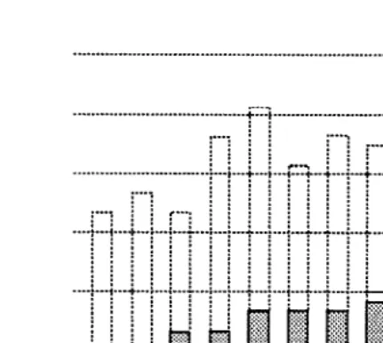
4. Set m(v)=ℓ(j+1)∀v∈Mj+1. Greedily reassign all tasks inRj+1and terminate. The reasoning behind the algorithm is as follows:
• The variableℓis always at most 6/ρtimes OPT, the optimum maximum load. In Step 1ℓis initialized to a trivial lower bound on OPT. We only increaseℓin Step 3, and then only if we find a large number of tasks(Rj+2)that can only be assigned to a small set of servers(Mj+2)—see Figure 1. This gives a lower bound of Rj+2/Mj+2 on OPT.
• If the number of levels is O(log n), we immediately have a competitive ratio of
O(log n). If the number of levels is larger, then there is some level j = O(log n) where Wj <Rj+2.
Fig. 2. In Step 4 Wj<Rj+2, and Rj+2/Mj+2< ρℓ/3, soRj+2is reassigned.
• If Rj+2/Mj+2 is small, then the number of tasks that have departed from servers in
Mj+2is enough to pay for reassigning all tasks inRj+1. See Figure 2. • With unlimited time, we could calculate an optimal reassignment ofRj
+1. However,
we do not need to. The theorem of Azar et al. [4] shows that greedily reassigningRj
+1 only increases the maximum load by at most OPT log n. Hence the maximum load is
O(jℓ+OPT log n)=O(OPT log n/ρ).
The following lemmas prove that the rebalance procedure halts correctly. Regarding termination, observe that the algorithm must halt in Step 2 onceℓ≥s.
To prove correctness, we begin by bounding the number of reassignments that occur during the sequence of task arrivals and departures. We define an operation to be either a task arrival and greedy assignment, a task departure, or an execution of the load-balancing procedure. We define a potential function8and say that the amortized number of reassignments for an operation is the actual number of reassignments plus the change in the potential.
LEMMA3. The amortized number of reassignments per departing task isρ. The
amor-tized number of reassignments per task arrival or load-balancing operation is at most zero.
PROOF. Let8 = P
vρ(m(v)−h(v)). The assignment of a task to a server cannot
increase the value of8, and the deletion of a task increases8by at mostρ.
Consider a reassignment done in Step 4 of the load balancing procedure with valueℓ. We show that the decrease in potential is at least Rj+1, the number of tasks
Let F= {v∈V |h(v)≥(j+1)ℓ}. We have
|F| ≤ Wj
ℓ ≤
Rj+2 ℓ .
Let E =Mj+2\F . For each server e ∈ E , h(e) < (j +1)ℓ. Upon resetting m(e)to (j+1)ℓ, the potential changes as follows:
18(e) = ρ[(j+1)ℓ−h(e)]−ρ[m(e)−h(e)] ≤ ρ[(j+1)ℓ−(j+2)ℓ]
≤ −ρℓ.
The potential associated with the servers outside of E is nonincreasing. The reassignment of the tasks above level j cannot increase the potential. Hence
−18 ≥ |E|(ρℓ)
≥ (ρℓ)(Mj+2− |F|) ≥ (ρℓ)
µ3R
j+2 ρℓ −
Rj+2 ℓ
≥ 2Rj+2.
Since Rj+2 = Rj+1−Wj+1 and Wj+1 ≤ Wj < Rj+2, we conclude−18≥ 2Rj+2 ≥
Rj+1.
LEMMA4. If task u has an edge to serverv, then m(v)≥h(u).
PROOF. The lemma is trivially true if u is assigned to serverv. Suppose u is assigned to serverw. When u was greedily assigned tow, columnvmust have had at least the same height asw, and hence m(v)was at least that height. The only way for m(v)to decrease is during a rebalancing, but since u has not been reassigned by assumption, that rebalancing must have left m(v)≥h(u).
THEOREM5. The Balance-A algorithm keeps the maximum on-line load within
13 log n/ρ times the optimum maximum load while performing ρm preemptive re-assignments over a sequence of m task departures.
PROOF. The bound on reassignments follows from Lemma 3 and standard arguments of amortized analysis.
Let OPT be the optimum maximum load. Observe that if there are a tasks that can only be placed on a given subset of b servers, then in any assignment of tasks to servers some server must have load⌈a/b⌉. Suppose that in Step 3 Rj+2/Mj+2 ≥ℓρ/3. By Lemma 4 the tasks inRj+2can only be placed on servers inMj+2, so OPT ≥ Rj+2/Mj+2, and
thereforeℓ≤6OPT/ρ.
Now assume that the rebalance algorithm terminates without reassigning tasks, so, for all j , Wj < Rj+2. Then the recurrence Rj+1 = Rj −Wj implies Rj+2 ≤ Rj/2 for
can be placed on one machine in level j . Hence there are at most 2 log n levels, so the maximum load is at most 12OPT log n/ρ.
On the other hand, assume a reassignment is done. Since j is chosen to be mini-mal, we have j +1 ≤ 2 log n. Consider the set of tasks that are in Rj+1 after the reassignment: these tasks were assigned greedily, without any task departures, so by the log n-competitiveness of the greedy algorithm for static load balancing [4], the maximum server load is at most (j +1)ℓ+OPT log n ≤ 13OPT log n/ρ after the reassignment.
Note that our algorithm belongs to a class of algorithms that does no preemptive rescheduling unless tasks depart the system. Hence we cannot hope to achieve a bound on the competitive ratio better thanÄ(log n), since the lower bound of Azar et al. [4] applies in the case of permanent tasks. This lower bound also applies to randomized algorithms in the same class.
2.2. Running Time of Balance-A. If a task arrives with a list of d edges to eligible servers, greedily assigning it takes2(d)time.
To implement the balance condition tests in Steps 2 and 3, the algorithm keeps
O(log n)arrays, one for each estimateℓthat may be tested. Each array stores the first
O(log n)values Wjℓ. Any tasks with height greater than the highest level are included in that level. As s doubles or halves we add new arrays for the minimum or maximum values ofℓ. The amortized cost is O(1)per task. To check the balance condition each successive value Rj is computed using the recurrence Rj+1 = Rj −Wj, R0 = s. An
analogous scheme is used for computing the values of Mj.
We show that the total time checking for violations of the balance condition is
O(log n). Suppose we begin Step 3 with some value of j andℓ. Since Wj(ℓ)′ ≥ R
(ℓ) j′+2 for j′ < j , we know that Wj(′2ℓ) ≥ R
(2ℓ)
j′+2for all j′ <⌊j/2⌋. Therefore ifℓis doubled and the procedure loops back to Step 2, it need only check the balance condition for
j′≥ ⌊j/2⌋. The value R⌊(2j/ℓ)2⌋can be computed in O(1)time from R(ℓ)j and the W values. Furthermore, R(ℓ)j+1≥ R⌊(2j/ℓ)2⌋+1, and every two times through the calculation loop of Step 2 the value of R decreases by 2. Combining these observations, we conclude that the total number of balance condition tests in Step 2 is O(log n), the the total time in Steps 2 and 3 is O(log n).
To implement rebalancing we need additional data structures. For each server we maintain a stack of the tasks on that server. Then the setRj+1can be found easily given the setMj+1. The setMj+1can be computed in O(log n+Mj+1)time by storing the
set of servers in a balanced binary tree ordered by m(v).
The cost of assigning a task to a server includes the basic cost of finding the minimum adjacent server plus the overhead of updating the above data structures. The overhead is
O(log n)worst-case. One entry must be updated in each of the O(log n)arrays storing the values Wj(ℓ). The balanced tree of servers can be appropriately modified in time O(log n) following updates to m(v). By Theorem 5 there are O(m)reassignments over m task arrivals and departures. Hence the amortized overhead per task arrival or departure is
The basic cost of greedy reassignments per task arrival or departure is O(d), where
d is sum of the degrees of all tasks currently in U .
THEOREM6. The Balance-A algorithm runs in O(d+log n)amortized time per task arrival and departure.
2.3. Balance-B. The Balance-B algorithm improves on the running time of Balance-A at the expense of a worse ratio in the load. It is based on the following observation. Suppose all tasks have identical degree b. Then the cost of computing a greedy reassign-ment of tasks can be amortized against the tasks that have departed by defining a second potential function8ˆ =b8and duplicating the proofs for the number of reassignments. It is easily seen that the amortized computation cost of an insertion remains O(b)while the amortized cost of a rebalancing is 0.
In general, tasks u∈U have arbitrary degree d(u). The Balance-B algorithm makes up for this by maintaining logδn different classes of tasks, where δ is a parameter between 2 and n. The tasks in class i have degree betweenδiandδi+1. Within each class independently we run the Balance-A algorithm.
THEOREM7. The Balance-B algorithm keeps the maximum on-line load within 13(log n) (logδn)/ρtimes the optimum maximum load, performsρm preemptive reassignments
over a sequenceσof m task arrivals and departures, and runs in total time O(m log n+ D(1+ρδ)), where D=P
u∈σd(u).
PROOF. The increase in the maximum load by a factor of logδn follows from there being O(logδn)classes. To prove the claimed running time, define a potential8i =δi+18
for each class i . When a reassignment is done, the drop in potential is at least the total degree of the reassigned tasks. When a task departs, the increase in potential is at mostρδ times its degree. Hence the total time spent on reassignments is O(Dρδ). After including
O(m log n)time for updating the arrays Wj(ℓ)during task arrivals and departures, and
O(D)time for initial (nonpreemptive) assignments of tasks, the total execution time is
O(m log n+D(1+ρδ)).
Note that no algorithm can improve on2(D)time unless it ignores some edges on tasks.
2.4. Weighted Load Balancing. Our algorithms are also applicable when each task u has a real size s(u) ≥ 1 and the load on a server is the sum of the sizes of the tasks assigned to that server. Let the height of a task be the sum of the sizes of tasks under it on its server. The load balancing procedure is essentially the same, although there is the small complication that tasks can lie across the boundary between levels. We redefine
Wj,Rj, Wj, and Rjto deal with weighted tasks as follows:
W(ℓ)
j = {u ∈U |h(u) < (j+1)ℓ& h(u)+s(u) > jℓ},
R(ℓ)
j = [
j′≥j
W(ℓ)
Wj(ℓ) = X
The definitions ofM(ℓ)j and Mj(ℓ)remain the same. We use the following modified load balancing algorithm. Let B be the maximum of the largest job size and the sum of the all job sizes divided by n.
+3and letvbe adjacent to u. In the unweighted case we had m(v) ≥ (j +3)ℓ, but now we know only that m(v) ≥ (j +2)ℓ, since
s(u)≤ B≤ℓ.
Using the potential function8=P
v∈V ρ(m(v)−h(v))we can repeat the proof of
Lemma 3 (with Rj+3 in place of Rj+2) and show that the amortized weighted cost of
reassignments charged to a departing task u isρs(u). That is, the total size of all tasks reassigned over a sequence of m task departures isρS, where S is the total size of all
departing tasks in the request sequence. If a is a lower bound on the size of a task, this bound implies that the total number of reassignments is at mostρS/a. In addition, we
can argue that the value ofℓ is always at least 8OPT/ρ. Following the reasoning of Theorem 5 we deduce the following theorem.
THEOREM8. The modified Balance-A algorithm achieves a competitive ratio of
25 log n/ρ while the total size of jobs reassigned is at mostρS, where S is the sum of sizes of all tasks that ever arrive.
To improve the running time, we can use the same partitioning scheme as before and easily derive an algorithm that achieves a ratio of 25 log n logδn/ρ and runs in time
O((m+ρS/a)log n+(1+δρS/a)D).
If bounds on the sizes of the tasks are known, however, then we can improve the running time as follows. Suppose a≤s(u)≤b for all tasks u. Partition the input tasks
into O(logδ(bn/a))classes such that task u is in class i if
In other words, partition the tasks based on number of edges per unit weight. The maximum value of the ratio is n/a, giving the bound on the number of classes.
For each class i define a potential function8ˆi=(δi+1/b)8. Now if, while rebalancing
class i , a collection of tasks having total size s is reassigned, then at most(δi+1/b)s edges
reassignments, and hence8ˆidecreases sufficiently to pay for examining the edges. The
increase in8ˆiwhen task u departs class i is given byρs(u)(δi+1/b)≤δρd(u). We have
the following.
THEOREM9. The modified Balance-B achieves a ratio of 25(log n)(logδbn/a)/ρ, runs
in total time O(m log n+D(1+ρδ)+min{ρs/a, ρδD}log n), and the total size of jobs
reassigned is at mostρS, where S is the sum of sizes of all tasks that ever arrive.
3. Network Flow
3.1. Intuition. Consider the EXACT-LOAD algorithm for the node kill game: whenever an item’s current edge is killed, reassign that item to the neighboring column with minimum load. Development of our algorithm for the node kill game was motivated by the proof of the following theorem.
THEOREM10. If there are no edge kills, EXACT-LOAD has a point score of O(n log2n).
PROOF. Consider the WATER-LEVEL algorithm, that is allowed to divide an item into pieces of arbitrary size, assigning the pieces to neighbors of the original item as desired. The height of a column is then the sum of the sizes of the pieces assigned to it. WATER-LEVEL redivides and reassigns items as frequently as necessary to maintain the following condition: if there is an item x with a piece on a column c and an edge to column c′, then h(c′)≥ h(c). (The WATER-LEVEL algorithm is actually the optimal off-line algorithm for minimizing the maximum load at all times.)
We compare EXACT-LOAD to the WATER-LEVEL algorithm, showing the follow-ing two points:
1. Let c be any column. The EXACT-LOAD height of c is always at most a factor
O(log n)larger than⌈hW(c)⌉, where hW(c)is the WATER-LEVEL height of c.
2. WATER-LEVEL incurs O(n log n)node kill points (where the point score of a column kill to c is⌈hW(c)⌉).
For point 2, fix a sequence of column kills. Assume there is some time t when the column killed does not have minimal height (under WATER-LEVEL’s assignment). Let
c be the first column later in the sequence that has minimal height. The height of c does
not increase after time t when the columns up till c in the sequence are killed, since by the definition of WATER-LEVEL, when the item pieces on those columns are reassigned, nothing can trickle down to c. Hence moving the kill of column c forward to time t does not decrease the point score. Hence there is a column kill sequence that achieves a maximum point score and always kills the current column of minimum height. For any such sequence WATER-LEVEL achieves a point score of O(n log n), since the i th last column killed has height at most n/i .
For point 1, let C be the set of columns whose WATER-LEVEL height is no more than hW(c), and consider the set I of items EXACT-LOAD has on columns in C. Note
that WATER-LEVEL assigns all pieces of each item in I to columns in C. Any x ∈ I
has at least one edge to a column in c1 ∈ C, and so if a piece of x were placed on a
The EXACT-LOAD assignment of items in I to columns in C is a greedy assignment, and the following analysis is similar to the proof that the greedy algorithm for on-line assignments is log n-competitive [4]. Order the items on columns of C under EXACT-LOAD’s assignment according to the time they were assigned. Partition each column into levels of⌈hW(c)⌉. Let Rj be the set of items in level j and above, and let Wj be
the set of items in level j . At least k ≥ |Rj|/hW(c)columns must have at least one
neighbor in Rj, since WATER-LEVEL can fit all items in Rj into one level of height
hW(c). By the definition of EXACT-LOAD, any such column must reach level j . This
implies Wj−1 ≥k⌈hW(c)⌉ ≥Rj. Hence the number of levels is O(log n).
3.2. The Ratio Algorithm. The disadvantage with EXACT-LOAD is that every time an item is reassigned, the entire edge set of that item must be scanned to find the lowest incident column. This is too much work in the case of network flow. To avoid the problem we use a different but related approach.
If a columnvhas height (or load) h(v)and initial degree dv, define r(v)=h(v)/dv
as the ratio ofv. There are two main differences between our algorithm for load bal-ancing and our algorithm for the node kill game. The first is that we perform greedy reassignments based on ratio rather than load.
The second difference is that it is too costly for items to monitor the precise ratio of neighboring columns. Define r =1/log n. If a columnvhas ratio r(v), define the
level l(v)= ⌊r(v)/r⌋. The algorithm maintains an estimated level el(v)which is known by all neighbors ofv. The estimated levels are updated as lazily as possible, subject to maintaining the relationship el(v)=l(v)or l(v)+1. This way many assignments or edge kills must occur on a column before its estimated level changes. Greedy assignments are based on estimated level. The algorithm of King et al. [11] also used greedy assignments by estimated level.
The ratio algorithm sometimes makes some columns inactive. Initially, any column vwith degree dv ≤log n is made inactive. When all the remaining neighbors of an item
have become inactive, the item is also inactive. From that time, whenever the item is subjected to an edge kill or node kill, it is reassigned to an arbitrary neighbor.
From now on we ignore inactive columns and items in the presentation of the algo-rithm. We can now describe the ratio algoalgo-rithm. It uses a rebalance routine (described below), which is closely related to the rebalanced routine of Section 2.
• A greedy assignment of an item u is as follows:
1. Assign u to the adjacent columnwof minimum estimated level. 2. Increment h(w). If r(w) > (el(w)+1)r , then increment el(w). 3. Perform a rebalance.
• Suppose the adversary kills the designated edge from u ∈ U to v ∈ V , forcing a
reassignment of u. Proceed as follows.
1. Decrement h(v). If r(v) < (el(v)−1)r , then decrement el(v). 2. Greedily assign u.
• To handle a column kill, process each item on the column as in the case of an edge kill.
3.3. Rebalancing. If an item on columnv has k items under it, we say its level is ⌊k/dvr⌋. Define the work at level j , Wj, to be the number of items in level j . The
residual work above level j , Rj, isPk>jWk.
We say the balance condition holds at level j if Rj+1 ≤ δWj. We will ensure the
balance condition always holds at all levels.
CLAIM1. If the balance conditions all hold, each column has level O(log1+1/δn).
We set the parameterδ=(n/m)εfor small constantε <1
2. Clearly a small value for δmeans the maximum ratio that can be attained is small.
Letγ =2+1/δ. The rebalance routine is as follows:
1. Let j be the minimum level such that Rj+1> δWj. If there is no such level, stop.
2. Let X be the set of items with level> j+1. Let E be the set of columnsvsuch that there is an edge from an item in X tov. Let F be the set of columns at levels≥ j+1. Finally, let Y =E∪F and dY =Pv∈Ydv.
3. If|X|/dY <r/γ, greedily reassign all items in X and stop.
4. If|X|/dY ≥ r/γ, make all columns in Y inactive. Greedily reassign all items that
were on those columns.
In Steps 3 and 4 the items to be reassigned are first removed from their columns, then assigned one by one, rebalancing after each assignment. Hence the balance conditions always hold, except perhaps for the effect of the last item assigned.
The complete analysis of the ratio algorithm appears in the next section. Here we outline the intuition for the above balance steps:
Step 3. The columns in Y have had many adversary edge kills, and though many were
originally too high for the items in X to be assigned to them, they aren’t any longer. The cost of the reassignments is charged to the edge kills.
Step 4. Many items can only go onto Y , so will become inactive when Y becomes
inactive. At most n items can ever become inactive, so the total degree of inactive columns is quite small. This keeps the point score on inactive columns low.
4. Analysis of the Ratio Algorithm. The analysis of the ratio algorithm is quite similar to that of the Balance-A algorithm. In particular, rebalancing work is charged to edge kills here, and to task departures there, in the same way.
Consider a rebalance at level j . Let F be the set of columns at levels≥ j+1. These columns are all full in level j , so we haveP
v∈Fr dv≤Wj <Rj+1/δ= |X|/δ.
Define a potential8as follows. For each columnvlet m(v)be the level of the highest adjacent item x. Then
8= 12X
v∈V
r dvmax{0,m(v)−el(v)} +12 X
v∈V
dvmax{0,r·el(v)−r(v)}.
LEMMA11. If the rebalance routine greedily reassigns in Step 3, the decrease in po-tential is at least|X|, so the amortized cost of the reassignments is≤0.
PROOF. The columns in Y that are not in F initially are at level j or lower, hence have estimated level at most j+1, and are all adjacent to at least one item in X . Since an item in X is at least at level j+2, the potential associated with each such column can be written asϕ≥ϕ0+12r dv. After the rebalancing, every item at level j+2 or higher
has been reassigned. Thus the new potential for each such column is at mostϕ0and the decrease is at least12r dv, so
A point is scored each time the ratio algorithm has to reassign an item because of a column kill or a rebalance. No points are scored for edge kills, however.
THEOREM12. The total number of points scored is O(mr log1+1/δn+nγ /r+√mn).
PROOF. First we consider points from column kills on active columns, and from re-assignments in Step 4 when columns become inactive. When an active column v is killed or becomes inactive, at most O(dvr log1+1/δn)items can be reassigned. Hence
the total number of these points is O(P
v∈Vdvr log1+1/δn)=O(mr log1+1/δn).
Secondly we consider points scored by node kills to inactive columns. The number of these points is at most dI, the total degree of columns that ever become inactive. Initially
dI ≤ n log n. By Step 4 of the rebalance routine, the number of items that become
inactive isÄ(r dI/γ ). At most n items can become inactive, so dI =O(nγ /r).
Thirdly we consider points scored in Step 3 of the rebalance routine. By Lemma 11, the number of these points is at most 12#edge kills. Finally, from Theorem 2 we know that #edge kills≤ O(√mn)+#points scored, and the theorem follows.
The following corollary gives parameters for the best performance of the ratio algo-rithm in terms of points scored in the game, if implementation cost were not an issue.
COROLLARY1. If we use the values r=pn/(m log n)andδ=1, then the total number
of game points is O(√mn log n).
4.1. Implementation of the Algorithm. To detect when to balance, we need a simple data structure for the columns. Keep arrays L[·] and R[·] of size log1+1/δn. Entry R[ j ]
contains the value of Rj and L[ j ] contains a linked list of the columnsvwith level j .
For each u∈U we maintain a set of A-lists and a B-list. The active columns adjacent to u are partitioned among O(log n)linked lists (the A-lists), one for each possible estimated level. List B is a list of active columns adjacent to u such that el(v)has decreased since
u was last reassigned. Whenever the estimated level of columnvchanges, the new value is broadcast to all items u to whichv has edges. The A and B lists of those items u are then updated, with columns moving between lists as appropriate. A column can be moved between lists in time O(1). When an item u is greedily assigned, it can find the adjacent column with smallest estimated level in O(log n)time by scanning to find the first nonempty list.
For eachv∈V we maintain a stack of the items assigned tov.
In the rebalance algorithm, the set X can be computed by popping items off the stacks of those columns in L[ j′] for j′≥ j+2. This takes time O(log n+ |X|). Given the set
X , the set of columns Y can be found as follows. Set F is easily found in time O(|F|) using the L[·] lists. Since|F| ≤ |X|from the analysis in Section 4, this takes time
O(log n+ |X|). Then examine each item x ∈X in turn. Scan the B list of x, and for each
columnvon the B list of x let Y =Y ∪ {v}. It is easy to verify that the set Y contains all columns that any element in X can be placed on.
THEOREM13. The total cost of implementing the ratio algorithm is O(m logm/nn+ n2log2+εn)for any constantε.
PROOF. We charge the implementation cost of the ratio algorithm to assignment points at a rate of O(log n)time units per reassignment. The theorem follows from substituting the values r =1/log n andδ=(n/m)εinto the reassignment bound of Theorem 12.
Whenever an item u is reassigned, its B list is reset to NIL, and otherwise it only grows, so B lists can be maintained in O(1)time per modification.
The cost of the rebalance algorithm is at most the cost of reassignments plus the sum of the sizes of the B lists of the elements. The latter size can be amortized against the operations that placed the columns on the B lists at O(1)per edge. So the total cost is simply the cost of reassignments.
There must be at least dvr reassignments or edge kills involving columnvto cause
a change in el(v). The cost of the subsequent broadcast is O(dv). Hence the cost of
updating lists is O(1/r)per reassignment.
When the height of a column changes, we update the values of R[·] as appropriate, and test for violations of the balance invariant. In addition, the column is moved between linked lists as needed. The total time for this is O(log n). A column changes its height only if a reassignment or kill has happened on it. Hence the work in updating R[·] and
L[·] can be amortized against reassignments and edge kills at a rate of at most O(log n) time units per reassignment. When an item is reassigned, it uses O(log n)time to make its greedy choice.
the point count, they do not affect the implementation cost (as long as mr log1+1/δn
remains the dominant term in Theorem 12).
THEOREM14. Network flow in a graph with N nodes and M edges can be computed in time O(M N logM/N N+N2log2+εN).
PROOF. Follows from Theorems 12 and 13, with r = 1/log n andδ = (n/m)ε, and
from Theorem 1.
4.2. Flow Operations. The number of flow operations is just O(log n)times the num-ber of points scored [8]. To determine the minimum numnum-ber of flow operations our algorithm can perform, while maintaining the running time given in Theorem 14, we use the slack in the choice of r , mentioned above. The smallest r can be made without increasing the running time is
r= (n/m)
1/2−ε/2
p
logm/nn
,
which makes mr log1+1/δn = nγ /r in Theorem 12 (the√mn term is insignificant).
Under this setting of r , the number of points is
(m/n)1/2+ε/2nqlogm/nn.
Substituting n = N2and m
= MN gives the following expression for the number of
flow operations of our algorithm on an N -node, M-edge graph:
# flow operations=M1/2+ε/2N3/2−ε/2qlogM/N N log N.
This matches the number of flow operations for the extended algorithm of King et al.
Acknowledgments. The authors gratefully acknowledge the contribution of Anna
Karlin in the early phases of this work.
References
[1] N. Alon. Generating pseudo-random permutations and maximum flow algorithms. Inform. Process.
Lett., 1990.
[2] Y. Azar, B. Kalyanasundaram, S. Plotkin, K. Pruhs, and O. Waarts. Online load balancing of temporary tasks. J. Algorithms, 22(1):93–110, 1997.
[3] Y. Azar, A. Broder, and A. Karlin. On-line load balancing. Theoret. Comput. Sci., 130(1):73–84, 1994. [4] Y. Azar, J. Naor, and R. Rom. The competitiveness of on-line assignments. J. Algorithms, 18(2):221–237,
1995.
[5] Y. Bartal, A. Fiat, H. Karloff, and R. Vohra. New algorithms for an ancient scheduling problem. J.
[6] J. Cheriyan and T. Hagerup. A randomized maximum flow algorithm. SIAM J. Comput., 24(2):203–226, 1995.
[7] J. Cheriyan, T. Hagerup, and K. Mehlhorn. Can a maximum flow be computed in o(mn)time? In Proc.
Internat. Colloq. on Automata, Languages, and Programming (ICALP 90), pages 235–248, 1990.
[8] J. Cheriyan, T. Hagerup, and K. Mehlhorn. A o(n3)-time maximum flow algorithm. SIAM J. Comput., 25(6):1144–1170, 1996.
[9] A. V. Goldberg and R. E. Tarjan. A new approach to the maximum flow problem. J. Assoc. Comput.
Mach., 35:921–940, 1988.
[10] R. L. Graham. Bounds for certain multiprocessing anomalies. Bell System Tech. J., 45:1563–1581, 1966. [11] V. King, S. Rao, and R. Tarjan. A faster deterministic maximum flow algorithm. J. Algorithms,
17(3):447–474, 1994.