On Boundary Damping for a Weakly Nonlinear Wave
Equation
Darmawijoyo
∗and W.T. van Horssen
†Abstract
In this paper an initial-boundary value problem for a weakly nonlinear string (or wave) equation with non-classical boundary conditions is considered. One end of the string is assumed to be fixed and the other end of the string is attached to a spring-mass-dashpot system, where the damping generated by the dashpot is assumed to be small. This problem can be regarded as a rather simple model describing oscillations of flexible structures such as suspension bridges or overhead transmission lines in a wind field. A multiple time-scales perturbation method will be used to construct formal asymptotic approximations of the solution. It will also be shown that all so-lutions tend to zero for a sufficiently large value of the damping parameter.
Keywords: wave equation, boundary damping, asymptotics, two-timescales pertur-bation method.
1
Introduction
There are a number of examples of flexible structures such as suspension bridges, overhead transmission lines, dynamically loaded helical springs that are subjected to oscillations due to different causes. Simple models which describe these oscillations can be expressed in initial-boundary value problems for wave equations like in [2], [5], [6], [10], [12], [13] or for beam equations like in [3], [4], [14], [15]. Simple models which describe these oscillations can involve linear or nonlinear second and fourth order partial differential equations with classical or non-classical boundary conditions. These problems have been studied in [2],
∗On leave from State University of Sriwijaya, Indonesia
†Department of Applied Mathematical Analysis, Faculty of Information Technology and Systems, Delft
[3],[4],[5], [6], [10], [12], [13] using a two-timescales perturbation method or a Galerkin-averaging method to construct approximations.
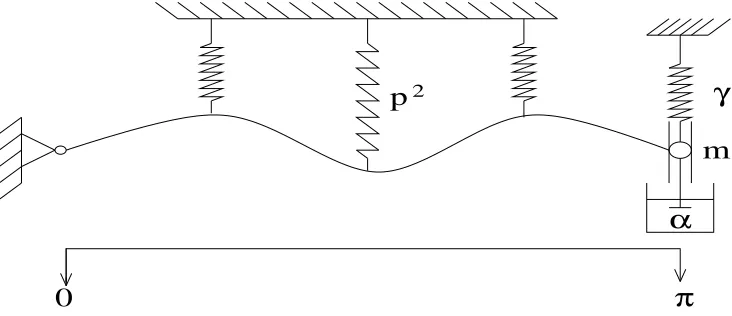
In most cases simple, classical boundary conditions are applied ( such as in [2], [3], [4], [10], [12], [13], [14]) to construct approximations of the oscillations. More complicated, non-classical boundary conditions ( see for instance [5], [6], [11], [15], [16], [17], [18]) have been considered only for linear partial differential equations. In this paper we will study an initial-boundary value problem for a weakly nonlinear partial differential equation for which one of the boundary conditions is of non-classical type. Asymptotic approximations of the solution will be constructed. In fact, we will consider the vibrations of a string which is fixed atx= 0 and is attached to a spring-mass-dashpot system atx=π (see also figure 1). This problem can be considered as a rather simple model to describe wind-induced vibrations of an overhead transmission line or a bridge (see [3,13]).
0
π
γ
m
α
p
2Figure 1: A Simple model of a suspension bridge.
It is assumed that ρ ( the mass-density of the string), T (the tension in the string), ˜m
(the mass in the spring-mass-dashpot system), ˜γ(the stiffness of the spring), ˜ǫ(the damping coefficient of the dashpot with 0<˜ǫ≪1 ), andp2 (for instance the spring constant of the the stays of the bridge) are all positive constants. Moreover, we only consider the vertical displacement ˜u(x,t˜) of the string, wherex is the place along the string, and ˜t is time. We neglect internal damping and consider the weight W of the string per unit length to be constant (W =µg , g is the gravitational acceleration). We consider a uniform wind flow, which causes nonlinear drag and lift forces (FD, FL) to act on the structure per unit length.
After some scalings, the equation describing the vertical displacement of the string is:
¯
utt−u¯xx +p2u¯=−µg+FD +FL. (1.1)
After some calculations (see also [13]) the following initial-boundary value problem is ob-tained as simple model to describe the wind-induced oscillations of the string(or bridge)
utt−uxx+p2u = ǫ
ut−
1 3u
3
t
u(0, t) = 0, t≥0, (1.3)
ux(π, t) = −ǫ(mutt(π, t) +γu(π, t) +αut(π, t)), t ≥0, (1.4)
u(x,0) = φ(x), 0< x < π, (1.5)
ut(x,0) = ψ(x), 0< x < π, (1.6)
whereφandψ are the initial displacement and the initial velocity of the string respectively, and wherep2, m, γ,andαare positive constants, and where 0< ǫ≪1. In this paper formal approximations (that is, functions that satisfy the differential equation and the initial and boundary values up to some order in ǫ) will be constructed for the initial-boundary value problem (1.2) - (1.6).
The outline of this paper is as follows. In section 2 we apply a two-timescales pertur-bation method to construct formal approximations for the solution of the initial-boundary value problem (1.2) - (1.6) and we analyze this solution. Also in section 2 we show that for all values of p2 mode interactions occur only between modes with non-zero initial energy
(up to O(ǫ) ). Moreover, it will be shown in section 2 that for α ≥ π2 all solutions tend to zero. In section 3 we make some remarks and draw some conclusions.
2
The construction of asymptotic approximations
To construct formal asymptotic approximations for the solution of the initial-boundary value problem (1.2) - (1.6) a two-timescales perturbation method (see [1,7,8]) will be used in this section. Since an approximation in the form of an infinite series will be constructed we will impose some additional conditions on the initial values in order to get a convergent series representation for which summation and differentiation may be interchanged. The additional conditions on the initial values are: φ(0) = φ′
(π) = φ′′
(0) = φ′′′
(π) = ψ(0) =
ψ′
(π) = ψ′′
(0) = 0, φ ∈ C4([0, π],ℜ), ψ ∈ C3([0, π], ℜ). By using a two-timescales perturbation method the functionu(x, t) is supposed to be a function ofx, t, andτ, where
τ =ǫt. We put
u(x, t) = v(x, t, τ;ǫ). (2.1)
By substituting (2.1) into the initial-boundary value problem (1.2) - (1.6) we obtain
vtt−vxx+p2v+ 2ǫvtτ +ǫ2vτ τ = ǫ
vt+ǫvτ −
1
3(vt+ǫvτ)
3
, (2.2)
0< x < π, t >0,
v(0, t, τ;ǫ) = 0, t≥0, (2.3)
vx(π, t, τ;ǫ) = −ǫ m(vtt(π, t) + 2ǫvtτ(π, t) +ǫ2vτ τ(π, t)) (2.4)
+γv(π, t) +α(vt(π, t) +ǫvτ(π, t))), t≥0,
v(x,0,0;ǫ) = φ(x), 0< x < π, (2.5)
vt(x,0,0;ǫ) +ǫvτ(x,0,0;ǫ) = ψ(x), 0< x < π. (2.6)
By expanding v into a power series with respect to ǫ aroundǫ= 0, that is,
and by substituting (2.7) into (2.2)-(2.6), and by equating the coefficients of like powers in
ǫ, it follows from the power 0 and 1 ofǫ respectively, that v0 should satisfy
vott−voxx+p
2v
o = 0, 0< x < π, t >0, (2.8)
vo(0, t, τ) = 0, t≥0, (2.9)
vox(π, t, τ) = 0, t≥0, (2.10)
vo(x,0,0) = φ(x), 0< x < π, (2.11)
vot(x,0,0) = ψ(x), 0< x < π, (2.12)
and that v1 should satisfy
v1tt−v1xx+p
2v
1 = vot −2votτ −
1 3v
3
ot, 0< x < π, t >0, (2.13)
v1(0, t, τ) = 0, t≥0, (2.14)
v1x(π, t, τ) = −(mvott(π, t) +γvo(π, t) +αvot(π, t)), t≥0, (2.15)
v1(x,0,0) = 0, 0< x < π, (2.16)
v1t(x,0,0) = −voτ(x,0,0), 0< x < π. (2.17)
The solution of (2.8) - (2.12) is given by
vo(x, t, τ) =
∞
X
n=0
Ancos(
p
λnt) +Bnsin(
p
λnt)
sin((12 +n)x), (2.18)
where λn = 12 +n
2
+p2, and where A
n and Bn are still arbitrary functions of τ which
can be used to avoid secular terms in v1. From (2.11), (2.12), and (2.18) it follows that
An(0) andBn(0) have to satisfy
An(0) =
2
π
Z π
0
φ(x) sin((1
2 +n)x)dx, (2.19)
Bn(0) =
2
π
Z π
0
ψ(x) sin((1
2 +n)x)dx, (2.20)
for n= 0, 1, 2,· · ·.
Next, we solve the initial-boundary value problem (2.13)-(2.17). In order to solve this problem we will make the boundary condition (2.15) homogeneous. For that reason we define the following transformation
v1(x, t, τ) =w(x, t, τ)−x(mvott(π, t, τ) +γvo(π, t, τ) +αvot(π, t, τ)). (2.21)
Substituting (2.21) into the initial-boundary value problem (2.13)-(2.17) we obtain
wtt−wxx+p2w = vot−2votτ −
1 3v
3
ot (2.22)
+x ftt(t, τ) +p2f(t, τ)
w(0, t, τ) = 0, t≥0, (2.23)
To solve the initial-boundary value problem (2.22) - (2.26) the eigenfunction expansion method will be applied. For that reason, the functionwis expanded into the Fourier series
w(x, t, τ) =
∞
X
n=0
wn(t, τ) sin((12 +n)x). (2.27)
The function as defined in (2.27) satisfies the boundary conditions at x = 0 and x = π. By substituting (2.27) into (2.22) the left-hand side of (2.22) becomes,
wtt−wxx+p2w=
, and by integrating the so-obtained equation with respect to x from 0 toπ, it follows that wn(t, τ) has to satisfy
. The last terms in the right-hand side of (2.29) (that is, the terms involving the sums) contain products of trigonometric func-tions. These products can be equal to sin(√λt) or cos(√λt), which are solutions of the homogeneous equation wntt+λnwn = 0. Obviously these products can give rise to secular
terms in w, and so in v1. To determine the terms in the products of the trigonometric
± √λn =
(2.30) - (2.34) we use a technique similar to the one used in [12].
By substituting (2.30) (that is,k+l−m =n,, ork−l−m−1 =n,ork+l+m+ 1 =n) into (2.31), or (2.32), or (2.33), or (2.34), by squaring the so-obtained equation twice, by rearranging terms and by using some elementary algebraic manipulations we find that the Diophantine-like problems (2.30) - (2.34) only have solutions for
1. n =k+l−m and √λn =
We rewrite (2.29) by taking apart those terms in the right-hand side of (2.29) that give rise to secular terms in w, yielding
wntt+ λn wn=
indicates that terms in this sum giving rise to secular terms are excluded. In order to avoid secular terms inw(and inv1) we have to take the coefficients of sin(
and cos(√λnt) in the right-hand side of (2.35) to be equal to zero, yielding allows us to truncate the infinite dimensional system (2.38) - (2.39) to those modes which have non-zero initial energy. To study system (2.38) - (2.39) in more detail we will use polar coordinates as defined by
¯
An = Rncos(φn), (2.40)
¯
Bn = Rnsin(φn), (2.41)
where Rn and φn are functions of τ.
After substituting (2.40) - (2.41) into (2.38) - (2.39) we obtain
for n = 0,1,2,· · ·. From (2.42) it is obvious that R′
n < 0 for α > π2. So for α > π2 all
solutions of (1.2) - (1.6) will tend to zero for increasing time t. When for instance only energy is initially present in the first two modes ( that is, Ro(0) 6= 0, R1(0) 6= 0, and
Rn(0) = 0 forn ≥2) a phase-plane analysis can be performed.
From (2.42) it then follows that Ro and R1 have to satisfy
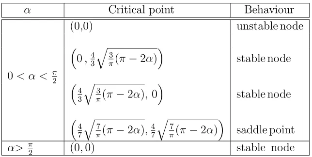
R′ two stable nodes, one unstable node, and one saddle point. For α > π2 the critical point is a stable node (see table 1).
Table 1: The behaviour of the critical points
α Critical point Behaviour
(0,0) unstable node
From the table it can readily be seen that if the damping parameter α is increasing (starting from α = 0) then the two stable nodes and the saddle point are moving to the unstable node. Forα = π
2 the four critical points coincide in (0,0), and for α >
π
2 a stable
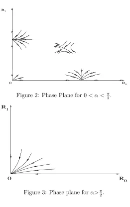
node occurs in (0,0). The behaviour of the solution of (2.44) - (2.45) can also be seen in figure 2 and in figure 3.
For 0 < α < π2 it can be seen in figure 2 that the solution (usually) will finally tend to a single mode vibration as t → ∞. For α > π2 it can be seen in figure 3 that the string vibrations will finally come to rest up to O(ǫ) as t→ ∞.
R0
R1
0
Figure 2: Phase Plane for 0< α < π
2.
R
R 0
1
0
Figure 3: Phase plane for α>π2.
some lengthy, but elementary calculations we obtain
wn (t, τ) =Fn(t, τ) +
∞
X
k=0 k6=n
gnk
A∗
kcos(
p
λkt) +B
∗
ksin(
p
λkt)
(2.46)
− 1
4
∞∗
X
k,l,m=0 k+l−m=n
− ∞
X
k,l,m=0 k−l−m−1=n
−1
3
∞
X
k,l,m=0 k+l+m+1=n
Sklm
4
X
i=1
cos(Ti
klmt+δklmi )
λn−(Tklmi )2
,
where Fn(t, τ) =Cn(τ) cos(
√
λnt) +Dn(τ) sin(
√ λnt),
A∗
n =mλnAn−γAn−α
√ λnBn,
B∗
n=mλnBn−γAn+α
gnk = 2π
k+1 2 n+1 2
2
(−1)k+n
λn−λk ,
Sklm =
√
λkλlλm
Q
i=k,l,m
p
A2
i(τ) +Bi2(τ),
T1
klm=
√ λk+
√ λl+
√
λm, δklm1 =αk+αl+αm,
Tklm2 =
√ λk+
√ λl−
√
λm, δ2klm =αk+αl−αm,
Tklm3 =Tkml2 , δklm3 =δkml2 ,
T4
klm=
√ λk−
√ λl−
√
λm, δklm4 =αk−αl−αm,
and where αn is defined as follows:
for A2
n+Bn2 = 0 :αn = 0,
for A2
n+Bn2 6= 0 : cos(αn) = √ Bn A2
n+B2n
, and sin(αn) = √An A2
n+Bn2
.
It should be observed thatwn still contains infinitely many free functionsCn andDnof
τ for n = 0,1,2,· · ·. These functions can be used to avoid secular terms in the solution of theO(ǫ2)-problem forv2. It is, however, our goal to construct a function ¯uthat satisfies the
partial differential equation, the boundary conditions, and the initial values up to order
ǫ2. For that reason Cn and Dn are taken to be equal to their initial values Cn(0) and
Dn(0) respectively. So far we constructed a formal approximation ¯u =vo+ǫv1 for u that
satisfies the partial differential equation, the boundary conditions, and the initial values up to orderǫ2. In [4,10,12,13] asymptotic theories are presented for wave and beam equations with similar nonlinearities. The formal approximations constructed for those problems were shown to be asymptotically valid, i.e., the differences between the approximations and the exact solutions are of order ǫon timescales of orderǫ−1
asǫ→0. It is beyond the scope of this paper to give the asymptotic analysis for the wave equation we discussed. We expect that the asymptotic validity of the constructed approximations can be shown in a way similar to the analysis presented in [4,10,12,13]. Finally it should be remarked that from these asymptotic theories it follows thatvo+ǫv1 andvo are both (orderǫ) asymptotic
approximations of the exact solution on timescales of orderǫ−1
.
3
Conclusions
α > π2 it also has been shown that all solutions tend to zero as t → ∞. For 0 < α < π2 it can be shown that the string system usually will oscillate in only one mode (up to O(ǫ)) as t→ ∞.
References
[1] A.H. Nayfeh, Perturbation Methods, Wiley, New York, 1973.
[2] J.B. Keller, and S. Kogelman, Asymptotic Solutions of Initial Value Problems for Nonlinear Partial Differential Equation, SIAM Journal on Applied Mathematics 18, 1970, 748 - 758.
[3] G.J. Boertjens and W.T. van Horssen, On Mode Interactions for a Weakly Nonlinear Beam Equation, Nonlinear Dynamics 17, 1998, 23 - 40.
[4] G.J. Boertjens and W.T. van Horssen, An Asymptotic Theory for A weakly Nonlinear Beam Equation With A Quadratic Perturbation, SIAM J. Appl. Math. Vol. 60, No. 2, 2000, pp. 602-632.
[5] Darmawijoyo and W.T. van Horssen, On the weakly Damped Vibration of A String Attached to A Spring-Mass-Dashpot System, 2001 (to appear).
[6] O. Morg¨¨ ul, B.P. Rao, and F. Conrad, On the stabilization of a cable with a Tip Mass, IEEE Transactions on automatic control, 39, no.10(1994,pp.2140-2145.
[7] J. Kevorkian and J.D. Cole, Multiple Scale and Singular Perturbation Methods, Springer-Verlag, New York, 1996.
[8] M.H. Holmes, Introduction to Perturbation Methods, Springer-Verlag, New York, 1995.
[9] Pao-Liu Chow, Asymptotic solutions of inhomogeneous initial boundary value prob-lems for weakly nonlinear partial differential equations, SIAM J. Appl. Math. Vol.22, No. 4, 1972, pp. 629 - 647.
[10] M.S. Krol, On a Galerkin - Averaging Method for Weakly nonlinear Wave Equa-tions, Math. Meth. Appl. Sci., 11(1989), pp. 649 - 664.
[11] N.J. Durant, Stress in a dynamically loaded helical spring, Quart. J. Mech. and Appl. Math., vol. xiii, Pt.2, 1960. pp. 251-256.
[12] W.T. van Horssen and A.H.P. van Der Burgh,On initial-boundary value prob-lems for weakly semi-linear telegraph equations. Asymptotic theory and application,
[13] W.T. van Horssen, An asymptotic Theory for a class of Initial - Boundary Value Problems for Weakly Nonlinear Wave Equations with an application to a model of the Galloping Oscillations of Overhead Transmission Lines, SIAM J. Appl. Math., 48 (1988), pp.1227 - 1243.
[14] F. Conrad, and ¨O. Morg¨ul, On the Stabilization of a Flexible Beam with a Tip Mass, SIAM J. Control Optim., 36 (1998), pp. 1962 - 1986.
[15] C. Castro, and E. Zuazua,Boundary Controllability of a Hybrid System Consist-ing in two Flexible Beams Connected by a Point Mass, SIAM J. Control Optim., 36 (1998), pp. 1576 - 1595.
[16] S. Cox, and E. Zuazua, The Rate at which Energy Decays in a String Damped at one End, Indiana Univ. Math. J., 44 (1995), pp. 545 - 573.
[17] B.P. Rao, Decay Estimates of Solutions for a Hybrid System of Flexible Structures, European J. App. Math., vol.4 (1993), pp. 303 - 319.