Abstract
This work deals with the numerical simulation on an unstructured mesh of the ignition and burning of an isolated fuel droplet modelled as a porous cylindrical wall. The reaction is assumed to be described by the equation A + B −→ P. The complexity of the physical model considered, including multi-scale feature and the presence of sti propagating fronts, justies manifold developments to overcome the diculties connected with corresponding simulations. Within this report, two recently developed methods are employed and compared. Both methods rely on nite volume approaches, but show distinct dierences in data-structures, choice of control volumes, meshing-strategy and even programming language.
c
1999 Elsevier Science B.V. All rights reserved.
Keywords:Droplet ignition; Finite volumes; Unstructured meshes; Roe; Gradient interpolation; Object-oriented numerics;
C++
1. Introduction
The numerical simulation of combustion phenomena continues to be a subject of great interest. Flame propagation processes play an essential role in most technical combustion devices, such as combustion engines, conventional power plants or house heating. Studying such processes to un-derstand the physical phenomena is a prerequisite for their optimization, thus having an important impact on a reduced production of pollutants in a wide range of technological applications.
However, the simulation of combustion problems faces diculties of several origins. A rst prob-lem is how to discretize and solve the full Navier–Stokes equations including reaction mechanisms eciently. These equations contain a hyperbolic part related to transport phenomena, a parabolic part due to diusion and viscosity as well as nonlinear and often sti source terms modelling chemical reactions.
∗Corresponding author.
A second problem is how to deal with the time and space multi-scale feature of the physical problem. The thinness of the reaction zone requires cells with very small scale lengths, at least in the normal direction. Since computational resources are restricted, adaptive, specially anisotropically adaptive meshing is very protable.
A third and throughgoing question, which is however not of major importance for the present studies, is the formulation of schemes, able to treat reacting ow problems with embedded shock waves. The development and improvement of upwind solvers, limiter formulations and extension to higher-order schemes is thus a continuous challenge.
According to the variety of diculties, many dierent methods and corresponding codes were de-veloped. Within the present paper, two numerical codes arising from dierent origins of development are presented and compared for the given physical problem. The aim is to evolve toward a unique code beneting of the advantages of both approaches.
2. Mathematical model
Considering an homogeneous mixture of N species A1; : : : ; AN and assuming that their combustion
process can be reduced to a one-step overall chemical reactionPN
i=1 iAi −→P N
i=1 iAi, the
conserva-tion equaconserva-tions can be expressed in the following general form:
@W
In the above equations, ; u; v; P; E are the density of the mixture, velocity components, pressure and total energy per unit volume, respectively. Yi and Mi represent the mass fraction and the molecular
mass of the species Ai. Q indicates the heat of the chemical reaction at a reference temperature T0. The components of the viscous tensor are
where B represents an algebraic function of the temperature and Ta the activation temperature of the reaction. Finally, for the problem to be closed, the equation of state has to be added to the above set:
where Pi is the partial pressure of Ai and R the perfect gas constant.
3. Sketch of the algorithms employed
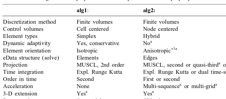
In the following the algorithmic approaches are referred to as alg1 and alg2. Both methods rely on nite volumes for logically unstructured grids. Their main purposes may be described in brief as in Table 1.
In the table, alg1 is especially designed for the physical problem described here, while alg2
corresponds to a multi-purpose development. Therefore, alg2 is still missing a reliable dynamic adaption tool as oered by alg1.
In the further sections of this paper, discretization methods of both algorithms will be described in more detail. However, before continuing, a short overview of the algorithmic structures is outlined.
3.1. The sequential algorithm, alg1
This code is especially designed for the physical problem described here and is thus highly opti-mized. As the vast majority of numerical methods for the simulation of complex physical problems, it relies on a procedural programming language, that is FORTRAN. The major advantage of such languages is the availability of very good compilers for Fortran as well as for C. Besides, For-tran codes are being developed since several decades and new versions are usually based on older ones.
As usual for sequential programming, the code splits up in subroutines, performing the dierent tasks. For the present system, we may summarize these as follows:
Table 1
Basic issues of algorithms employed.∗1: in development or unused property within the current paper
alg1: alg2:
Discretization method Finite volumes Finite volumes Control volumes Cell centered Node centered
Element types Simplex Hybrid
Dynamic adaptivity Yes, conservative Noa
Element orientation Isotropic Anisotropic∗1a eData structure (solve) Elements Edges
Projection MUSCL, 2nd order MUSCL, second or quasi-thirda order Time integration Expl. Runge Kutta Expl. Runge Kutta or dual time-stepa
Order in time Second First or second
Acceleration None Multi-sequencea or multi-grida
3-D extension Yesa Yesa
Programming Sequential Objective
Programming language FORTRAN C++
• Advance in time. This part performs the discretization and integration for an interval.
• Mesh adaptation. This task performs a rearrangement by discrete operations.
The latter two items are interchangeable: that is a mesh rearrangement is performed in cycles after a set of (or a single) time step(s).
To conclude, we may say that procedural languages are very useful for the solution of a specic problem. However, the corresponding algorithms are less exible. In practice, this results in large numbers of program versions when solving dierent physical problems.
3.2. The objective algorithm, alg2
The aim of this development is the construction of a reliable platform for a variety of applications. At the site of the authors these range from ship-hydrodynamics to the simulation of the structure of detonation waves.
Dealing with the same grid types, data structures and iteration methods, a very high partition of the code is independent from a concrete physical problem to be simulated. The advantage of objective programming in this context is that it allows a very consequent dissection in modules for logical and physical parts of the program.
The whole software is therefore split in three major programming levels:
• Basic storage classes. These classes include dynamic data handling. These objects are independent of the kind of problems treated and thus do not even relate to the solution of dierential equations.
• Basic functionality. These objects include the solution concepts, mesh generators, handling of data structures as well as some utility routines and hardware-dependent loop iterators.
• The physical level. Herein a user may allocate data and create the processing methods for his specic application. All calls to procedures are virtual. Using a method of the basic functionality suitable for its application does not require knowing much about these.
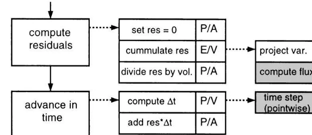
Fig. 1. Sketch of a simple explicit time step. P: pointwise, E: edgewise, A: automatic, V: virtual. Grey elds: dependent on a specic application.
that is, regardless of the variables in use, the corresponding method is always available. For the projection of variables from the nodes to the cell interfaces, a choice of automatic methods is available. The user of the system may thus concentrate on the computation of the time step length and the ux-formulation for his application (Fig. 1).
The dotted arrows indicate virtual function calls. These require an additional amount of computa-tional time. To minimize this overhead it is useful to provide a sucient amount of computacomputa-tional work within the virtually called methods. Therefore, these methods contain loops for subsets of points or edges, respectively. Since data are passed between subsequent virtual calls, it is not useful to perform the inner loops over all points or edges, but only for moderate-sized groups, thus saving memory.
The one-step time integration is the simplest version. However, all other explicit integration strate-gies are implemented in the same way. Therefore, once a ux and a time-step calculation for a physical problem is formulated, other more complex integration methods are accessible as well.
4. Finite volume schemes and discretizations
4.1. The nite volume scheme
Integration of system (1) over a control volume Vi and Gauss divergence formulas leads to
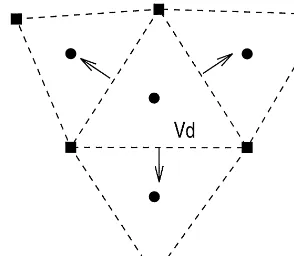
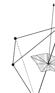
Fig. 2. Cell–centred control volume.
The discrete form of the above equations for a control volume Vd reads
W
Since unstructured grids do not oer a natural ordering of nodes and elements, an articial or-dering, i.e., a data structure is required. Further on an element of the data structure will be called a molecule. To perform a time step for the equation given above, the discrete residual Res;Vd has
to be constructed upon such molecules. Introducing the discrete ux functions and v for the
nonviscous and viscous uxes yields
Res;Vd=
where nr(Vd) is the number of molecules contributing to the residual, VVd is the corresponding
volume, nj˜(j) represents the outward normal vector and Aj˜(j) the area of the control interface supported by a molecule ˜j(j).
alg1 employs cell-centred control volumes. Corresponding molecules are the common edges be-tween two neighbouring cells and the normal vectors are the normals ni˜(i) to these interfaces (Fig. 2).
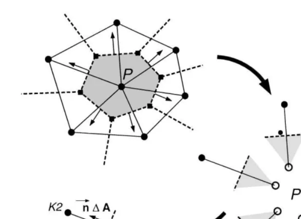
Fig. 3. Decomposition of a 3-D control volume and edge-based molecule.
A mixed discrete-analogue edge-based data structure is employed. For each edge of the mesh the addresses of the two ending nodes K1; K2 and the control interface area-normal vectors nA
between the control volumes of both nodes are stored.
For a ux evaluation at a cell interface, a projection of the variables stored at the cells (alg1), respectively nodes (alg2), onto the corresponding cell interfaces is required. The formal spatial order of the algorithm is determined by this projection. Both algorithms employ MUSCL projection.
For the cell-centred approach of alg1, the cell gradients are evaluated by minimizing the quadratic functional
LVd(X; Y) =
X
k∈K(Vd)
|WVd+ (xk−xVd)X + (yk−yVd)Y −Wk|
2
;
where K(Vd) is the set of indices of neighbourhood cells that have a common edge or vertex with the control volume Vd, (xVd; yVd) and (xk; yk) are respectively the barycentre coordinates of cells Vd
and Vk.
Nodal gradients of the conservative variables, required for the projections to be performed for
alg2, are obtained by a Green–Gauss-type integration at the control volumes themselves:
∇WVd =
1
VVd
nr(Vd) X
j=1
Wj˜(j)nj˜(j)Aj˜(j): (5)
Fig. 4. Decomposition of a 2-D control volume and edge-based molecule.
4.2. Flux formulations for the hyperbolic part
For the present simulations, both schemes employ Roe’s approximate Riemann ux function. Consider the hyperbolic part of Eqs. (1):
Wt+Fnv(W)x+Gnv(W)y= 0 (6)
classically called the Euler equations.
The hyperbolic contribution to the residual, requires the evaluation of the term:
Z
where j˜(j) is calculated upon the left- and right-hand side projected variables Wl and Wr. Rather
than regarding an edge ˜j(j), we will thus refer to the left and right sides of the cell interface l and
r. Roe proposed the following particular choice of (Wl; Wr) [6]:
where A( ˜W ;nlr) is an average Jacobian matrix constructed to satisfy the following properties, which
traduce respectively the consistency with jump conditions, positiveness and convective ux denition, (i) Fnv(Wr;nlr)−Fnv(Wl;nlr) =A( ˜W ;nlr) (Wr−Wl);
(ii) A( ˜W ;n) is diagonalisable with real eigenvalues, (iii) (W; W)·n = F
simple to evaluate. For details we may refer here to [2].
4.2.2. Entropy correction
One disadvantage of Roe’s linearization is that the resulting approximate Riemann solution consists of only discontinuities which can lead to nonentropic shocks. In this case, entropic modication is required. The approach used here due to Harten and Hyman [4] consists of introducing a rarefaction wave wherever the Roe scheme produces nonadmissible shocks. A correction is required, if the left and right sonic eigenvalues of same type have dierent signs, while representing a rarefaction:
l=(Wl)¡0¡ r =(Wr):
This situation may correspond to a nonphysical shock. To overcome the problem, the eigenvalues are modied. Depending on the simplication chosen, one of the following modications are required:
∗
4.3. Formulation of diusive terms
The discretization of the diusive ux contributions in the context of nite volume methods require the discretization of terms of the following type:
Z
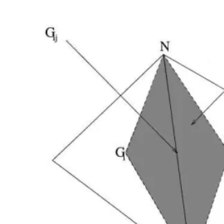
Fig. 5. Diamond shaped co-volume.
towards the entropy solution was proved under some stability condition and some requirements on the mesh: the angles of each triangle must be lower than 1
2.
The algorithms presented here use two-step formulations to compute the ux contribution. In a rst step, the gradients required at the cell interfaces are computed. In a second step an ordinary nite volume type discretization is performed. For the computation of gradients, Green–Gauss-type integrations are employed for both algorithms.
4.3.1. Diamond shaped co-volume
The cell-centred approach of alg1 uses an edge centred co-volume, as sketched in Fig. 5. The gradients, which are supposed to be constants on the co-volume Cdec, are computed upon the values of the data on the nodes Gi, Gj, N, and S as follows:
To obtain the values at a node N of the mesh, a specic linear interpolation based on the set of cells sharing the vertex N is employed, ensuring weak consistency of the scheme (see [3]).
4.3.2. Direct nite volume method
Since already required for the higher-order projections, alg2 provides a set of conservative gradi-ents at the nodes, as computed in Eq. (5). These gradigradi-ents are thus reused for the formulation of viscous uxes.
In a rst step, average gradients are obtained at the cell interfaces. Following the left–right notation, where the stateslandr correspond to the nodes at both the ends of the edge regarded, the preliminary gradient reads:
∇W˜lr = 1
Fig. 6. Continued
Since in the direction of the edge a central formulation of the gradients is possible, the preliminary conservative gradient may be corrected in order to reduce the range of inuence:
∇Wlr =∇W˜lr+
where Llr is the length of the corresponding edge, mlr the unit vector aligned with.
The primitive gradients, required for the evaluation of the terms 10, are then computed at the cell interface employing dierentiation rules. For example, the gradient of the speed u in x-direction reads:
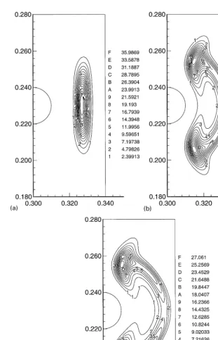
Fig. 8. alg2: reaction rate isolines of the mixture at dierent time steps t1; t2; t3:
Fig. 9.alg1: mass fraction isolines of fuel at timet3:
Fig. 11. alg2: mass fraction isolines of the fuel at timet3:
that K has to be divided into 4 sons, and that each of these sons has to be divided into 4m−1 sub-triangles. The algorithm is then based upon a multi level hierarchical tree data structure.
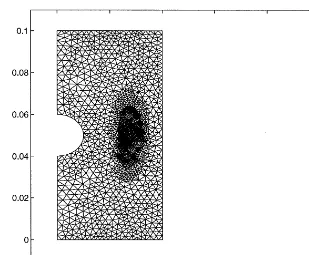
6. Numerical experiments
For the comparison of the two algorithms described above, the simulation of the ignition and burning of a fuel droplet is considered. Therefore a simplied combustion model was used consisting of three species, including a one-step overall chemical reaction A + B −→ P. The fuel indicated by the symbol A reacts with the oxidizer B to form a new species P. The density of the mixture, initially consisting only of the oxidizer (YF(x; y;0) = 1, YO(x; y;0) = 0), was assumed to be (x; y;0) = 1. The ow was initially at rest having a temperature of T(x; y;0) = 300 K. On the droplet surface the mass fraction of the fuel was set to YF;drop= 1 so that YO;drop = 0.
The leakage of the fuel through the droplet surface is obtained by relating the conditions specied on the droplet surface to the maximum pressure Pmax inside the computational domain. Initiated by a temperature ofT = 1100 K at the right boundary of the domain the mixture was ignited. For this pla-nar wall the Neumann condition has been applied to the mass fractions@YF=@n=@YO=@n= 0. On the boundaries at the top and the bottom of the domain, the velocities were assumed to beu= 0; v= 0. The values of constants taken are as follows: = 1:4; Cv= 717 J kg
−1
K−1;
0 = 0:03 kg m
−1 s−1;
Fig. 12. alg2: mass fraction isolines of the oxidizer at time t3:
Fig. 14. Temperature isolines foralg2at time t3:
7. Conclusion
Two dierent methods, developed at dierent sites, have been studied to simulate the problem of a droplet ignition. Both codes rely on nite volume approaches and employ a simplied version of Roe’s approximate Riemann solver. Beside these similarities, both methods dier signicantly. It is thus interesting to note that the results of both methods are in good agreement, although they were not even applied on the same computational mesh.
Upon further development we plan to combine the advantages of the dierent methods. Concerning the discretization and meshing techniques, a 3-D extension of the methods is a challenging problem. Adaptive or not, both meshing concepts employed for the present studies where isotropic. Due to the high computational complexity, such concepts are not useful in 3-D. Anisotropic concepts, by way of contrast, most often result in additional diculties for the discretization of viscous terms, crucial for the problem presented.
References
[1] F. Benkhaldoun, T. Fernandez, B. Larrouturou, P. Leyland, A dynamical adaptive method based on local renement and unrenement for triangular nite-element meshes : Preliminary results, Rapport de Recherche no. 1271, INRIA, 1990.
[2] T. Buard, J.M. Herard, Methodes de resolution pour les systemes hyperboliques en forme conservative sur maillage non structure, Rapport EDF, HE-41=90:43, 1990.