24 (2000) 273}295
Animal spirits, technology shocks and the
business cycle
Mark Weder*
Department of Economics, Humboldt University Berlin, Spandauer Str. 1, 10178 Berlin, Germany
Abstract
This paper presents a two-sector growth model which allows indeterminacy to occur at relatively mild degrees of increasing returns. It is shown that economies of scale need only be present in one sector of the economy, e.g. the investment good producing sector. This new feature of the model builds on evidence that was recently reported by Basu and Fernald (1997), (Journal of Political Economy 105, 249}283) and others. The time series that are generated by the model have properties that are comparable to the real U.S. postwar data. The sunspot driven model is also able to solve some puzzles of business cycle research which standard Real Business Cycle models have not been able to explain. ( 2000 Elsevier Science B.V. All rights reserved.
JEL classixcation: E00; E32
Keywords: Sunspots; Technology shocks; Economic #uctuations; Dunlop}Tarshis-puzzle
1. Introduction
The last few years have witnessed a revival of business cycle models in which beliefs of agents (or animal spirits) have played a leading role in explaining economic #uctuations.1 Most of these models involve strong economy-wide increasing returns to scale in order for sunspot equilibria to exist. In a recent paper, however, Basu and Fernald (1997) present evidence that returns to scale
*E-mail: [email protected].
1See, for example, Farmer (1993), Farmer and Guo (1994), Gali (1994) and Schmitt-Grohe (1997). 0165-1889/00/$ - see front matter ( 2000 Elsevier Science B.V. All rights reserved.
are far from evenly distributed across the U.S. economy. In particular, they report that scale economies are present mainly in the domain of durable goods production. In the nondurable goods sector of the U.S. economy evidence of increasing returns to scale cannot be found. Similarily, Harrison (1996)"nds evidence of modest increasing returns to scale in the U.S. investment good sector. The consumption goods sector, however, appears to operate under constant returns.
The innovation of this work is to demonstrate that these empirical "nd-ings can be used within a two-sectoral optimal growth model with market imperfections to generate non-uniqueness of rational expectations equilibria. Moreover, it will be shown that returns to scale in the consumption good sector are theoretically irrelevant for obtaining indeterminacy. Indeter-minacy arises at returns to scale of around 1.07 in the investment sector alone.2
Although the debate on business cycles was revived as a result of the new literature on self-fulxlling expectations, it is indisputable that these recent developments have failed to produce a widely accepted paradigm as of today. The principal problem in this new literature is the dependency on degrees of scale economies and market power that are not suggested by (most) recent empirical studies. Benhabib and Farmer (1996), however, are able to show that by working with a two-sector optimal growth model the extent of increasing returns that is needed to obtain indeterminacy can be reduced signi"cantly.3
The main di!erence between their work and the model presented here is that Benhabib and Farmer do not consider any asymmetry of scale economies of the sort reported by Basu and Fernald (1997). A further distinction is that they study an economy with perfect competition and sector speci"c externalities whereas the model developed here is characterized by Cournot competiton and internal returns to scale. Unlike the work by Gali (1994), however, in the present model the variable markup is not a function of the composition of demand but rather dependent on the degree of economic activity in each sector. The market structure allows to obtain indeterminacy in the case of increasing marginal costs where returns to scale originate from overhead costs only.
The paper proceeds as follows: Section 2 presents the model. The economy's steady state and the dynamics will be derived in Section 3. In Section 4 the model is calibrated. This is followed by two exercises; the "rst will establish parameter constellations at which indeterminacy is possible and the second
2See Harrison (1996) for a related result.
will compute model statistics to assess the model's business cycle properties (Sections 5 and 6). Section 7 concludes the paper.
2. The model
The economic model developed is a two-sector extension of a baseline Real Business Cycle model as in, for example, King et al. (1988). Markets for investment goods and consumption goods are characterized by oligopoly.4
2.1. The household
It will be assumed that the economy consists of a representative household. The household supplies labor and capital services to the"rms on competitive markets. A representative agent has expected lifetime utility
E
C
+= t/0bt;(C
t,lt)DIt
D
, (1)where;( . ) is instantaneous utility,C
t is a consumption index,lt leisure time,
bthe discount factor andI
tthe set of information available att. The following
speci"c functional form for periodic utility is assumed:
;(C
t,¸t)"logCt#
B
1#sl1t`s with s40, (2)
where Bis a constant. Consumption of the households is de"ned by a CES-aggregator over all di!erentiated goods which are normalized to unity:5
C
The aggregator for the investment good,I
t, is de"ned as:
The period-by-period budget constraint of the household is given by
P
14Gali (1995) also includes oligopoly in the Real Business Cycle framework.
wherep
c,c,t (pi,i,t) is the price of the consumption (investment) goodc(i). Both
prices are taken as given to the households.w
tis the nominal wage.
Further-more, the household receives pro"t income from all existing "rms P
t. It also
owns the stock of capitalK
t, which is rented out to the"rms at the rental price
q
t. Factor markets are perfectly competitive. Households are endowed with one
unit of time per period which they can either use for leisure or work¸
t:
1"¸
t#lt. (6)
The consumer's capital holdings evolve as
K
t`1"(1!d)Kt#It, (7)
wheredis the rate of depreciation. The household maximizes Eq. (1) subject to Eqs. (3)}(7). As is well known for this class of models, maximization can be conducted as a two step procedure. The conditional demand on consumption goods can be derived in the"rst step as
C
which has a constant price elasticity. Herep
c,t,(:10ptc,@(ct,t~1)dc)(t~1)@tis the exact
price indices for the consumption goods. The analogous investment good demand becomes
Given these conditional demands, it is possible to derive the intertemporal optimality condition for the household. In symmetric equilibrium, which is the only case to be considered in this work, the household buys the same amount of every product and the prices of all goods equal. The price of the consumption goods in equilibrium is used as the numeraire and, without loss of generality, is normalized to unity. The budget constraint transforms into
C
t#ptIt"wt¸t#qtKt#Pt. (10)
p
t can be interpreted as the relative price of investment goods in symmetric
equilibrium.
The second step of the household's optimization program consists of comput-ing the optimal path of spendcomput-ing and workcomput-ing. Each household chooses a se-quence MC
t,¸t,Kt`1N=t/0 subject to K0 and to the distribution of technology
innovations (see below). The household's optimal decisions must satisfy
as well as satisfying the household's budget constraint and the transversality condition. Eq. (11) describes the household's consumption-leisure trade o!and Eq. (12) is the standard intertemporal optimality condition.
2.2. Thexrms
One signi"cant modi"cation of conventional Real Business Cycle modelling is considered: consumption and investment goods are produced in two distinct sectors. Households can move their labor and capital services freely and without costs between the two sectors. It is assumed that product markets are oligo-polistic.
2.3. The consumption goods sector
The part of the economy that produces consumption goods consists of subsectors or markets of measure one, each producing a di!erentiated product.6
There areN
c,t"rms supplying their single goodjevery periodtin their subsectorc.
Each"rm supplies its product on the market under the assumption of Cournot competition. Costless endogenous entry and exit of "rms will be allowed in order to drive pure pro"ts to zero.
Firmjhas access to the following increasing returns technology:
>
c,j,t"Cc,j,t"Zt(Kac,j,t¸1~c,j,ta)c!/, (13)
withK
c,j,tcapital input,¸c,j,tlabor input, and/overhead costs.Ztis the state of
technology which evolves as7
logZ
t`1"ologZt#zt`1, 04o(1 andN(0,p2z).
Given the assumption on the form of competition and Eq. (8), the "rm's program can be written in the speci"c Cournot form
maxP
subject to its production function. p
c,j,t is the price of the "rm's good and
C
c,~j,tis the supply of all other"rms on the market which is taken as given for
every"rmj. The cost function of a"rm is given by
C(w
6Basically both sectors of the economy are the same in structure. Therefore, only the sector that is discussed"rst is described in detail.
where A is a constant. Marginal costs are decreasing (increasing) for
The last equation equalizes marginal revenues and marginal costs. At every period in time the number of active "rms is implicitly determined by a zero pro"t condition.
In symmetric equilibrium,N
c,tCc,j,t"Cc,t"Ct,Nc,t"Ntandpc,j,t"pc,t"1
hold, where the last equality follows from the normalization that was already made in the previous subsection. Inserting the optimal pricing rule into the zero pro"t condition yields in symmetric equilibrium
C
t#1 is the inverse of the markup in the consumption goods
sector. Note that the markup is decreasing in t which implies that a high substitutability of the input goods translates into a low degree of market power. The markup is also decreasing in the number of "rms. That is, the model predicts a countercyclical pattern of the markup. This behavior is supported by empirical evidence summarized by Rotemberg and Woodford (1991).8By com-bining the optimal markup rule with the conditional demand for labor, it is possible to derive the (equilibrium) wage rate as
w
The rental rate of capital is given by
q
2.4. The investment goods sector
There areM
i,t"rms supplying their respective investment goodjin subsector
i.9The market structure and the production technology in the investment goods
8See also Burda (1985).
sector are essentially the same as in the consumption goods sector. Each"rm supplies its product under the assumption of Cournot competition. It operates with increasing returns technology
>
i,j,t"Ii,j,t"Zt(Kai,j,t¸1~i,j,ta)g!C, (19)
whereK
i,j,tand¸i,j,tare the"rm's capital and labor input andCare overhead
costs. In symmetric equilibrium, the zero pro"t condition is given by
I
The optimal inverse factor demands are implicitly determined in symmetric equilibrium by
From the zero pro"t condition, it is easy to show that the internal increasing returns to scales are equal to the markup.
3. The solution method
The following section describes the dynamics of the economy near its steady state. Since the Second Welfare Theorem does not apply because of the existing market power, the dynamics cannot be derived by means of the social planner problem. Therefore, the necessary and su$cient "rst order conditions are log-linearized.10The model reduces to the three-dimensional dynamical system
C
E[p(whereJis 3]3. The eigenvalues ofJmust be evaluated at the steady state. The system contains one predetermined variable, the stock of capital, KK t, one endogenous nonpredetermined variable, p(
t, and one exogenous
nonpredeter-mined variable,ZKt. Thus, if all eigenvalues of J are inside the unit circle, the
rational expectations equilibrium is non-unique. This will be analyzed in the following section. The calibration method will be applied to check if indetermin-acy has realistic relevance.
4. Calibration
Parameter value determination will follow in the Real Business Cycle tradi-tion. Steady-state values of the model will be matched with estimates of average growth rates and great ratios. A baseline model structure will be de"ned. Without setting"xed values for all variables, the regions of realistic calibrations will be shown.
To calibrate the model as close as possible to established Real Business Cycle theory, parameters are set as proposed in existing studies. Quarterlydis equal to 0.025 anda, the capital share, is set at 0.30.
Basu and Fernald (1995) report estimates for increasing returns from 1.00 to 1.26. However, their preferred point estimate is 1.03. In their work the regression was restricted by assuming that returns to scale are the same over the economy. In a more recent work, Basu and Fernald (1997), in turn show that economies of scale are largely heterogenous across the economy. For durable goods manufac-turing, they report signi"cant increasing returns.11 For the production of nondurables, on the other hand, (insigni"cant) diminishing returns are reported. A similar picture arises in Harrison (1996). Based on these results, it will be assumed that the consumption sector in the present model displays close to constant returns. This is an assumption which will not be changed throughout this paper.
The markups over marginal cost are given by
1
MC"
N t!1#N
for the consumption goods sector and by
P
MC"
M
h!1#M
for the investment goods sector. The last two equations each possess one degree of freedom. For example, if one"xes both the markup andtin the consumption goods sector, the number of steady state"rmsN is uniquely determined. The same holds for the investment goods sector. Existing empirical literature does
not o!er information concerning the magnitude of the elasticity of substitution in Eqs. (3) and (4). In models of monopolistic competition, the elasticity of substitution and the markup are interdependent since they are exactly inverse to each other. This is not the case in under Cournot competition. Basu and Fernald report markup margins from 1.00 to 1.26. Morrison (1990) reports the markup to be around 1.14. In the remainder, it is simply assumed that the inverse oft(h) always equals the markup as a normalization.
Kydland and Prescott (1990) report that total consumption expenditures amount to 80% of output net of government expenditures. If only expenditures on nondurables and services are considered, the ratio falls to 68%. In the present model, the ratio of consumption to overall expenditures is generally "xed at 80% which is the same value as in Benhabib and Farmer (1996).12The steady-state rate of return can be represented by
r"q
p!d"
1 b!1.
An annual return of four percent conveys a discount rate ofb+0.99.13 This assumption is standard in Real Business Cycle models.Cand/do not appear in the linearized version of the economy.
5. Indeterminacy
5.1. Indeterminacy zones
Indeterminacy is present in the model as long as both roots of the matrixJare inside the unit circle. A numerical solution is used here. Table 1 considers the parameters which are not changed in the analysis unless otherwise noted.
Table 1 implies that the markup in the consumption sector is essentially one. This value is also the measure of increasing returns.14The assumption can be justi"ed by comparing it to the empirical work by Basu and Fernald (1997) and Harrison (1996). The other calibrations were discussed in the previous section. Table 2 displays regions for indeterminacy for alternative values of scale economies in the investment goods sector. The labor market follows the Hansen (1985) construct, that is s"0. Marginal costs are constant in both sectors:
c"g"1.00, thus, for h(1, the markup is variable. The table shows that the
12This is done by adjusting the preference parameterB. The main results of the paper carry over to alternative assumptions on the consumption share.
13Harrison (1996) calibrates the discount factor instead. This minor di!erence shows up in very small numerical deviations to her work in Tables 2}5.
Table 1 Parameters
¸ C/> a t d b
1/3 0.80 0.30 0.9999 0.025 0.99
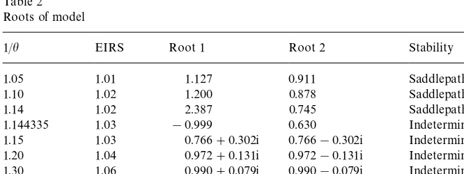
Table 2 Roots of model
1/h EIRS Root 1 Root 2 Stability
1.05 1.01 1.127 0.911 Saddlepath stable
1.10 1.02 1.200 0.878 Saddlepath stable
1.14 1.02 2.387 0.745 Saddlepath stable
1.144335 1.03 !0.999 0.630 Indeterminacy
1.15 1.03 0.766#0.302i 0.766!0.302i Indeterminacy 1.20 1.04 0.972#0.131i 0.972!0.131i Indeterminacy 1.30 1.06 0.990#0.079i 0.990!0.079i Indeterminacy 1.40 1.08 0.995#0.061i 0.995!0.061i Indetermiancy 1.50 1.10 0.996#0.051i 0.996!0.051i Indeterminacy
present model does not require unrealistic scale economies in order to produce indeterminacy.15The model is indeterminate at increasing returns to scale in the investment goods sector of 1.15. Existing one-sector models which were sum-marized in Schmitt-Grohe (1997) require much higher scale economies. This result alone indicates an improvement over previous work. Moreover, the presence of returns to scale is limited to one sector only. The economy-wide returns to scale (EIRS) amount to 1.03.16 It is generally the case that the eigenvalues do not change if other assumptions are made on the returns to scale in the consumption sector. The indeterminacy result depends solely on the scale economies that are present in the investment goods sector. Finally, if it had been assumed instead that the markup is constant, for example through monopolistic competition and by a "xed number of "rms, the constancy of marginal costs would exclude the possibility of indeterminacy.17
15The matrixJcontains a third root which equals the parameterowhich is not reported in the
tables.
16These are computed by weighting the respective sectoral returns to scale by the respective output share.
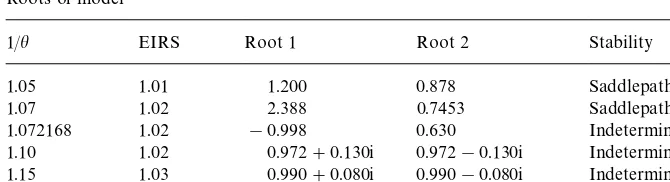
Table 3 Roots of model
1/h EIRS Root 1 Root 2 Stability
1.05 1.01 1.200 0.878 Saddlepath stable
1.07 1.02 2.388 0.7453 Saddlepath stable
1.072168 1.02 !0.998 0.630 Indeterminacy
1.10 1.02 0.972#0.130i 0.972!0.130i Indeterminacy 1.15 1.03 0.990#0.080i 0.990!0.080i Indeterminacy 1.20 1.04 0.994#0.061i 0.994!0.061i Indeterminacy
Table 4 Roots of model
1/h EIRS Root 1 Root 2 Stability
1.15 1.03 1.248 0.862 Saddlepath stable
1.18364 1.04 !0.991 0.629 Indeterminacy
1.20 1.04 0.904#0.226i 0.904!0.226i Indeterminacy
gis set equal 0.90.
Table 3 repeats the analysis for decreasing marginal costs, in particular
g"1/h.18By assuming decreasing marginal costs the returns to scale that are
needed to produce indeterminacy can be reduced even further. They must be around 1.07 in the investment sector alone. This value is well within the reported scale economies in Basu and Fernald (1998). Furthermore, it is marginally lower than what is reported in Harrison (1996) who considers a model which is closer in essence to the original Benhabib and Farmer (1996) approach in which returns to scale are the result of externalities. The economy-wide scale econo-mies are a mere 1.015. It is also of interest that Basu (1995) points out the case that observed scale economies do not arise from decreasing marginal costs (as in Farmer and Guo, 1994, or Benhabib and Farmer, 1996), but rather result from overhead. Table 4 shows that decreasing marginal costs are not generally needed in the present model: indeterminacy may arise with an upward sloping marginal costs curve (herec"0.90).
Until now I have demonstrated the results in an indivisible labor environment only. In Table 5 it is assumed that parametersvaries. The left-hand column of
(Table 5
Alternative labor supply elasticities
1/h EIRS s ELS
1.072 1.015 !0 R
1.121 1.026 !1 2
1.159 1.032 !2 1
1.202 1.040 !5 0.40
1.224 1.045 !10 0.20
1.242 1.049 !20 0.10
the table indicates the minimum returns to scale that are needed to obtain indeterminacy. All other remaining parameters are the same as in Table 3. For lower labor supply elasticities (ELS), the scale economies needed are higher but are still low when compared to other models. Therefore, the model does not rely on outright unrealistic labor supply elasticities in order to produce indeterminacy. Until now only the average returns to scale have been reported. However, the apparent aggregate returns to scale might be higher due to (strong) procyclical-ity of sectoral inputs. A useful check on the accuracy of the claim that returns to scale are indeed modest in the above calculations would be to estimate the aggregate returns by regressing aggregate output on the bundle of aggregate inputs.19The data is taken from a simulated model with 2000 realizations that is driven by animal spirits shocks alone.20It is assumed that parameters are set the same as in Table 2. The returns to scale in the investment sector are 1/h"1.10 which implies average aggregate returns of around 1.02. The regression is as follows
ln>
t"b1(alnKt#(1!a)ln¸t)#et.
This is equivalent to the regressions run by Basu and Fernald (1995). The procedure yields an estimatebK1"1.12. The returns increase by the amount of 0.10, however, they can still be considered modest. Other possible calibrations yield similar results.
In sum the most signi"cant aspect of the present model is that it is able to yield an indeterminate solution for largely realistic parameter constellations. In face of recent critique on the animal spirits approach to business cycles, a criti-cism which centered on the implausible assumptions that were made on the degree of market imperfections, the present model is able to set out a structure that allows for the existence of indeterminacy at realistic measures. Moreover,
19I thank one referee for suggesting this procedure.
these increasing returns need only be present in the investment goods sector. In the present economy increasing returns to scale are due to overhead costs, a feature which is also supported empirically. The model must still be evaluated to see how well it is able to replicate stylized business cycle facts, however. This will be carried out in the next section. Before doing so, an economic reasoning for the indeterminacy result will be given.
5.2. The economic intuition behind the indeterminacy result
The economic intuition for indeterminacy in the model can be formulated as follows: suppose agents expect (unrelated to any changes in economic funda-mentals) that the future return to capital is going to be high. This will induce a shift of current resources towards investment goods. However, the expecta-tions must be supported in the new equilibrium, namely at a higher return to capital. There are several ways to generate an increase in the rental rate at a higher level of economic activity. All of these cases can be accounted for in the present in model. First of all, it is assumed that increasing returns are present in the economy. If returns to scale are the result of a falling marginal cost curve and not only of overhead costs, an increase in investment goods production can straightforwardly convey a higher capital return. Second, an increase in invest-ment demand generates also an in#ow of "rms which implies a fall of the markup (see for example Eq. (18)). If the markup is countercyclical in the investment goods sector for any given stock of capital, the labor input and the return to capital can potentially increase at higher activity. That is, even when marginal costs are constant or increasing, indeterminacy is possible. Third, labor moves freely across sectors. If the production of investment goods rises, labor is shifted into the investment goods sector and the return of a given stock of capital increases.21 If all of these features are combined or work seperately, the return to capital can increase with economic activity. For all these situation to arise, the returns to scale in the consumption goods sector are irrelevant.
6. Business cycle properties
6.1. Population moments
The model must still be judged on how good it can replicate the variability of the di!erent aggregate macroeconomic time series behavior. In accordance with
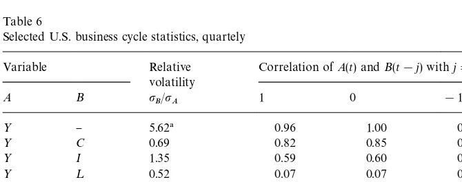
the Real Business Cycle approach, the generated model data will be compared with real data. Table 6 reports population moments for the U.S. economy.
The well-known stylized business cycle fact can be observed: consumption #uctuates less than output and investment displays a greater volatility than output. The right part of the table gives cross correlations of the variables. All variables peak with output. The bottom line displays the autocorrelation of output growth which measures the persistence of aggregate output. The process of "rms'entry and exit takes on an important role in the present model. The procyclical behavior of net business formation is well documented for the U.S. economy in Audretsch and Acs (1991) or Campbell (1995), and are further discussed in Devereux et al. (1996).
6.2. Model moments
Sunspot equilibria are de"ned as rational expectations equilibria in which cyclical behavior arises in response to arbitrary random events that do not have an e!ect on the fundamental equilibrium conditions of the economy. Once the sequence of sunspots is generated, the law of motion of the economy, which
Table 6
Selected U.S. business cycle statistics, quartely
Variable Relative Correlation ofA(t) andB(t!j) withj" volatility
A B pB/pA 1 0 !1
> } 5.62! 0.96 1.00 0.96
> C 0.69 0.82 0.85 0.84
> I 1.35 0.59 0.60 0.57
> ¸ 0.52 0.07 0.07 0.06
> = 1.14 0.72 0.76 0.74
> IS 0.56 0.74 0.81 0.77
> CS 0.70 !0.72 !0.89 !0.73
*> } 0.99! 0.37 1.00 0.37
The table is taken from King et al. (1988)} deviations from common linear trend, quarterly, 1948:I}1986:IV. Variable de"nitions:>"real gross national output,C"consumption expenditure on nondurables and services,I"gross"xed investment,¸"total workers employed (Household Survey) and="gross average hourly earnings of production workers.IS"investment expendi-tures share ("xed invesment) andCS"consumption expenditures share (nondurables and services) are from Kydland and Prescott (1990), deviations from HP trend, quarterly, 1954:I}1989:IV.
*>"output growth which is taken from Christiano and Todd (1996) whose data set covers the 1947:I}1995:I period.
below includes technology shocks, is given by
t`1 is an i.i.d. expectational error which can be interpreted as animal
spirits (see Farmer, 1993 or Woodford, 1991).
In the remainder of this section the sample moments of the model will be reported for various calibrations. First, a baseline calibration is speci"ed which will not be altered unless noted (Table 7). The value of s implies that the intraperiod utility is equivalent to that in the Hansen}Rogerson model. The t calibration follows the notion that increasing returns are only present in the investment goods sector.
Table 8 reports a version of the model with very low scale economies (1.10) and which is driven by an i.i.d. animal spirits shock sequence only. The table
Table 7
Variable Relative Correlation ofA(t) andB(t!j) withj" volatility
Deviations from linear trend. Variable de"nitions:>"output (>
t"Ct#ptIt),C"consumption expenditures, I"investment (p
indicates two major counterfactual characteristics of the model. First, consump-tion and labor productivity are countercyclical. Second investment is much too volatile. Along other lines, the model performs reasonably well. Most notably it generates highly autocorrelated time series and realistic relative volatilities of the remaining variables. The expenditures shares move in correct directions: the investment share is strongly procyclical and aggregate expenditures on con-sumption goods are countercyclical.
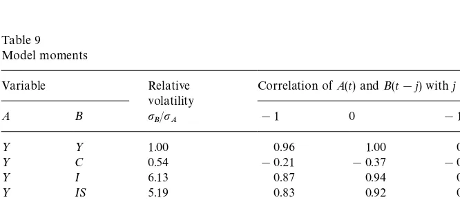
The countercylical behavior of consumption in two sector models is well-known from the Benhabib and Farmer (1997) survey. However, this fact is not limited to multiple equilibria models. Hu!man and Wynne (1997) report the very same result for a two sector Real Business Cycle model with technology shocks. Only the introduction of adjustment costs allows the latter authors to obtain procyclical consumption. Other potential solutions that will be discussed in the remainder of this work are higher returns to scale, a variable markup and, combined with greater scale economies, technology shocks. To make Hu!man and Wynne's (1997) result visible in the present model, Table 9 reports the time series of the model when it is driven by i.i.d. technology shocks alone (o"0). The calibration is the same as in the preceeding version. Surprisingly, Tables 8 and 9 o!er a very similar picture of the model economy. Moreover, at least at low increasing returns to scale, consumption appears to be negatively correlated with output if technology is i.i.d. Also, as in Hu!man and Wynne (1997), aggregate labor productivity is countercyclical.
Benhabib and Farmer (1996) point out that a su$ciently higher degree of returns to scale allows the generation of procyclical consumption in their model. Therefore, Table 10 considers the case of a model economy observes higher
Table 9 Model moments
Variable Relative Correlation ofA(t) andB(t!j) withj" volatility
A B pB/pA !1 0 !1
> > 1.00 0.96 1.00 0.96
> C 0.54 !0.21 !0.37 !0.47
> I 6.13 0.87 0.94 0.96
> IS 5.19 0.83 0.92 0.94
> CS 1.29 !0.83 !0.92 !0.94
> ¸ 1.30 0.83 0.92 0.94
> P 0.54 !0.21 !0.37 !0.44
¸ P 0.38 !0.54 !0.69 !0.74
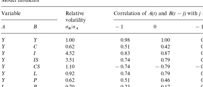
Table 10 Model moments
Variable Relative Correlation ofA(t) andB(t!j) withj" volatility
A B pB/pA !1 0 !1
> > 1.00 0.98 1.00 0.98
> C 0.62 0.51 0.42 0.41
> I 4.52 0.83 0.87 0.89
> IS 3.51 0.74 0.79 0.81
> CS 1.10 !0.74 !0.79 !0.81
> ¸ 0.92 0.74 0.79 0.81
> P 0.62 0.51 0.46 0.41
¸ P 0.70 !0.23 !0.17 !0.11
*> *> 1.00 0.20 1.00 0.20
returns to scale of 1.20. This is the same extent of returns to scale as in Benhabib and Farmer's (1996) simulated model except that scale economies are present in both sectors in theirs. Animal spirits are the only source of#uctuations. The dynamics of consumption are substantially altered: the contemporaneous cor-relation of consumption with output becomes positive and the relative volatility is very close to what is found in data. This result conforms to the Benhabib and Farmer (1996) model, although returns to scale are limited to one sector of the economy here. Labor productivity is procyclical. Also, hours and productivity are mildly negatively correlated. The prediction of the model is quite close to the value of!0.34, as reported Canova (1998) for the U.S.economy.22This is the socalled Dunlop-Tarshis puzzle which states that real wages (productivity) and labor input move essentially uncorrelated to each other (see Tarshis, 1939; Dunlop, 1938). The model is thus able to solve an arduous puzzle of business cycle research which standard Real Business Cycle models have not been able to.23
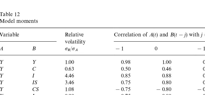
Introducing persistent technology innovations into the last model version helps to generate an even better match (o"0.90). Both shock sequences are uncorrelated and of equal size. As can be seen from the last line in Table 11, output persistence increases and resides at the level that is reported by Christiano and Todd (1996). Also, the low zerocorrelation of labor and produc-tivity is similar to the predicted one in mentioned empirical studies.
22McGrattan (1994) who HP"ltered the data reports a correlation of!0.20.
Table 11 Model moments
Variable Relative Correlation ofA(t) andB(t!j) withj" volatility
A B pB/pA !1 0 !1
> > 1.00 0.99 1.00 0.99
> C 0.63 0.50 0.43 0.40
> I 4.56 0.85 0.86 0.89
> IS 3.55 0.77 0.81 0.83
> CS 1.11 !0.77 !0.81 !0.83
> ¸ 0.93 0.77 0.81 0.83
> P 0.63 0.50 0.43 0.40
¸ P 0.70 !0.21 !0.15 !0.09
*> *> 1.00 0.34 1.00 0.34
Table 12 Model moments
Variable Relative Correlation ofA(t) andB(t!j) withj" volatility
A B pB/pA !1 0 !1
> > 1.00 0.98 1.00 0.98
> C 0.63 0.50 0.46 0.40
> I 4.46 0.85 0.88 0.90
> IS 3.46 0.75 0.80 0.82
> CS 1.08 !0.75 !0.80 !0.82
> ¸ 0.90 0.75 0.80 0.82
> P 0.63 0.55 0.51 0.47
¸ P 0.70 !0.24 !0.19 !0.13
*> *> 1.00 0.14 1.00 0.14
investment goods, the (relative) markup declines. This makes investment goods even more attractive and consumption goods are substituted. Only if returns to scale are high, the induced wealth e!ect creates a positive correlation.
Table 13 reports the e!ect of the slope of marginal costs onto consumption's procyclicality. It shows the output-consumption correlation for alternative gs while holding "xed 1/h"1.20. Procyclical consumption is easier to obtain if marginal costs are decreasing. One may interprete this"ndings as being similar to the wealth e!ect that operates in a pure RBC model with technology shocks. It is this e!ect } a downward shift of the cost function } that generates procyclical consumption in that model. A falling marginal costs schedule oper-ates similarly.
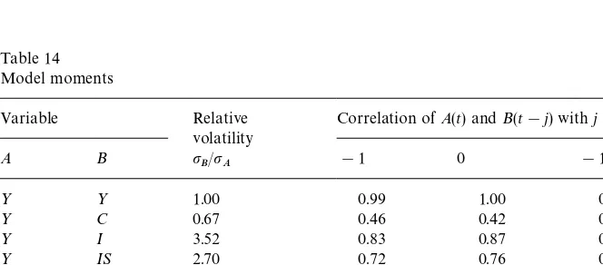
Finally, an even higher degree of returns to scale is assumed: c"1.50, combined with constant marginal costs g"1.00 e.g. the case of a variable markup where increasing returns are solely the result of overhead costs. This amount of scale economies correponds to the Baxter and King (1991) model. Animal spirits are the only present driving variable (Table 14). The above extent
Table 13 Model moments
g Correlation ofC(t) and>(t)
1.20 0.43
1.15 0.18
1.10 !0.06
1.00 !0.36
0.90 !0.77
Table 14 Model moments
Variable Relative Correlation ofA(t) andB(t!j) withj" volatility
A B pB/pA !1 0 !1
> > 1.00 0.99 1.00 0.99
> C 0.67 0.46 0.42 0.36
> I 3.52 0.83 0.87 0.89
> IS 2.70 0.72 0.76 0.79
> CS 0.94 !0.72 !0.76 !0.79
> ¸ 0.94 0.72 0.76 0.79
> P 0.67 0.46 0.82 0.36
¸ P 1.40 !0.21 !0.27 !0.32
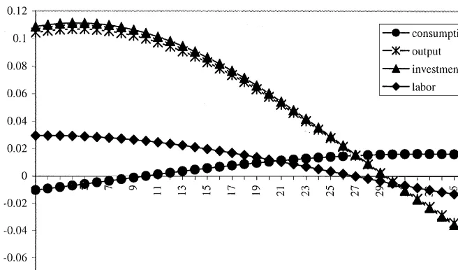
Fig. 1.
of returns to scale is admittedly unrealistically high. However the model predic-tions display close similarities to the ones that have been reported in Table 6 for the U.S. economy.
Overall, in terms of business cycle statistic, the model is not necessarily worse than existing (one sector) Real Business Cycle models. Most features of data can be replicated.
6.3. Impulse response dynamics
24See also Farmer and Guo (1994) for the analysis of the one-sector animal spirits model. persistence is due to endogenous propagation for the white noise animal spirits shock.24 The model provides an example of an economy with the ability to signi"cantly propagate temporary shocks.
7. Conclusion
In this paper a stochastic two-sector growth model is developed which allows indeterminacy to occur at very mild degrees of increasing returns. Furthermore, it is shown that it is su$cient that these economies of scale are present in only one sector of the economy. This feature of the model builds on empirical evidence that was recently reported by Basu and Fernald (1997) and Harrison (1996). The size of the returns to scale in the consumption good sector is theoretically irrelevant in generating indeterminacy. The model is also able to solve some puzzles of business cycle research which standard Real Business Cycle models have not been able to. Namely, the introduction of animal spirits at modest returns to scale allows the generation of a low and negative contem-poraneous correlation of hours and productivity. Considering more standard measures of the business cycle, such as the relative volatility of aggregate variables and comovements, the model performs equally as well as existing Real Business Cycle models. Finally the paper provides an example of a model which o!ers a strong endogenous propagation mechanism.
Acknowledgements
I am indebted to Michael Burda for his guidance. I would like to thank Jess Benhabib, Dalia Marin, Ellen McGrattan, Harald Uhlig, Rolf Tschernig, two anonymous referees and seminar participants at Heidelberg, EUI-Florence (EEA Summer School), SUNY at Stony Brook and Toulouse (EEA '97) for valuable comments. All remaining errors are mine. This research was supported by the DFG-Sonderforschungsbereich 373 &Quanti"cation and Simulation of Economic Processes'.
References
Audretsch, D.B., Acs, Z.J., 1991. New-"rm startups, technology and macroeconomic#uctuations. WZB Discussion Paperd91-17.
Basu, S., Fernald, J.G., 1997. Returns to scale in U.S. production: estimates and implications. Journal of Political Economy 105, 249}283.
Basu, S., Fernald, J.G., 1995. Are apparent productivity spillovers a"gment of speci"cation error? Journal of Monetary Economics 36, 165}188.
Baxter, M., King, R.G., 1991. Productive externalities and business cycles. Federal Reserve Bank of Minneapolis Discussion Paperd53, Institute for Empirical Macroeconomics.
Benhabib, J., Farmer, R.E.A., 1997. Indeterminacy and sunspots in Macroeconomics. In: Woodford, M., Taylor, J. (Eds.), Handbook of Macroeconomics, forthcoming.
Benhabib, J., Farmer, R.E.A., 1996. Indeterminacy, and sector speci"c externalities. Journal of Monetary Economics 37, 421}443.
Burda, M.C., 1985. New evidence on real wage-employment correlations from U.S. manufacturing data. Economics Letters 18, 283}285.
Campbell, J.R., 1995. Entry, exit technology, and business cycles. Rochester Center for Economic Research Working Paperd407.
Canova, F., 1998. Detrending and business cycle facts. Journal of Monetary Economics 41, 475}512.
Christiano, L.J., Todd, R.M., 1996. Time to plan and aggregate#uctuations. Federal Reserve Bank of Minneapolis Quarterly Review 20, 14}27.
Devereux, M.B., Head, A.C., Lapham, B.J., 1996. Aggregate#uctuations with constant returns to specialization and scale. Journal of Economic Dynamics and Control 28, 627}656.
Dunlop, J., 1938. The movement of real and money wage rates. Economic Journal 48, 413}434. Farmer, R.E.A., 1993. The Macroeconomics of Self-Ful"lling Prophecies. MIT Press, Cambridge. Farmer, R.E.A., Guo, J.T., 1994. Real business cycles and the animal spirits hypothesis. Journal of
Economic Theory 63, 42}72.
Gali, J., 1994. Monopolistic competition, business cycles and the composition of aggregate demand. Journal of Economic Theory 63, 73}96.
Gali, J., 1995. Non-Walrasian unemployment#uctuations. NBER Working Paperd5337. Hansen, G.D., 1985. Indivisible labor and the business cycle. Journal of Monetary Economics 16,
309}328.
Harrison, S.G., 1996. Production externalities and indeterminacy in a two sector model: theory and evidence. Department of Economics, Northwestern University, Mimeo.
Hu!man, G.W., Wynne, M.A., 1997. The role of intratemporal adjustment costs in a multi-sector economy. Federal Reserve Bank of Dallas, Journal of Monetary Economics, forth-coming.
King, R.G., Plosser, C.I., Rebelo, S.T., 1988. Production growth and business cycles I: the basic neoclassical model. Journal of Monetary Economics 21, 195}232.
Kydland, F.E., Prescott, E.C., 1990. Business cycles: real facts and a monetary myth. Federal Reserve Bank of Minneapolis, Quarterly Review 14, 3}18.
McGrattan, E.R., 1994. A progress report on business cycle models. Federal Reserve Bank of Minneapolis, Quarterly Review 18, 2}16.
Morrison, C., 1990. Market power, economic pro"tability and productivity growth measurement: an integrated structual approach. NBER Working Paperd3355.
Perli, R., 1997. Indeterminacy, Home production and the business cycle: a calibrated analysis. Journal of Monetary Economics, forthcoming.
Rotemberg, J., Woodford, M., 1991. Markups and the business cycle. In: Blanchard, O.J., Fischer, S. (Eds.), NBER Macroeconomics Annual 6. MIT Press, Cambridge, pp. 63}129.
Schmitt-Grohe, S., 1997. Comparing four models of aggregate#uctuations due to self-ful"lling expectations. Journal of Economic Theory 72, 96}147.
Tarshis, L., 1939. Changes in real and money wage rates. Economic Journal 49, 150}154. Uhlig, H., 1995. A toolkit for analyzing nonlinear dynamic stochastic models easily. Tilburg
Weder, M., 1998. Fickle consumers, durable goods and business cycles. Journal of Economic Theory 81, 37}57.
Weder, M., 1996. Self-ful"lling prophecies and business cycles in a two-sector stochastic growth model. Mimeo, Humboldt University, Berlin.