for rules that use forecasts of inflation rather than just contemporaneous inflation. Under the uncertainty considered, the magnitudes of the efficient response coefficients tend to increase. © 2000 Elsevier Science Inc.
Keywords: Monetary policy rules; Uncertainty; Potential output
JEL classification: E52; E31; E17
I. Introduction
Research on monetary policy rules has demonstrated the efficacy of simple rules. For example, Rudebusch and Svensson (1998) illustrate that efficient simple rules have similar stabilization properties to more complex optimal rules. Levin et al. (1998) show that simple rules are more robust than optimal rules to model uncertainty. Clarida et al. (1997) demonstrate that simple rules appear to explain how policymakers actually behave. In addition to their efficacy, simple rules may be widely used in practice because they
Economics Department, Reserve Bank of New Zealand, Wellington, New Zealand
Address correspondence to: Dr. B. Hunt, Reserve Bank of New Zealand, Economics Department, 2 The Terrace, P.O. Box 2498, Wellington, New Zealand.
The views expressed in this paper are those of the authors and do not necessarily represent the views of the Reserve Bank of New Zealand. The author’s would like to thank an anonymous referee, Ralph Bryant, and participants at a workshop on ‘Monetary Policy Under Uncertainty’, held at the Reserve Bank in June 1998, for comments on an earlier version of the paper. Any remaining errors and omissions are the responsibility of the authors.
provide policymakers with a comprehensible framework to communicate the factors motivating their actions.
Common to many of these simple rules is their dependence on measures of the economy’s supply capacity or potential output. There is considerable uncertainty about the economy’s level of potential output, however, because it is unobservable. Policymakers must rely on estimates derived from observed data. Several recent studies have examined the implications of potential output uncertainty for response coefficients in simple policy rules. In Smets (1999), observation errors associated with an unobserved-components model of potential output lower the magnitude of response coefficients in an optimal Taylor rule. Considering the implications of statistical uncertainty around a Phillips curve estimate of the natural rate of unemployment, Wieland (1998) finds that the uncertainty reduces the magnitude of optimal policy rule coefficients. However, Isard et al. (1998), find the opposite result when considering the effect of uncertainty about the natural rate of unemployment on efficient Taylor rule coefficients. The difference in results appears to arise from the nature of the policymaker’s errors. In Isard et al., the errors are generated from a real-time updating process that leads to errors that are correlated through time and with the cycle. The optimal control techniques employed in Smets (1999) and Wieland (1998) do not allow for uncertainty of this nature.
We generate the inflation-output variability frontiers, as introduced in Taylor (1979), to investigate the effects of a particular characterization of potential output uncertainty on the performance and characteristics of three classes of simple efficient policy rules. Stochastic simulations of the Reserve Bank of New Zealand’s macroeconomic model are used to trace out the efficient frontiers. The three classes of rules considered are inflation-forecast-based rules; Taylor (1993) rules; and inflation-forecast-based rules that include the contemporaneous output gap. We choose this set of rules because they have been examined extensively in the literature and appear to be used in practice.1 The characterization of uncertainty about the economy’s supply capacity that we consider embodies the notion that the techniques employed by policymakers to estimate potential output will often lead to errors that are serially correlated and depend on the state of the business cycle.
Not surprisingly, the performance of all three classes of rules deteriorates under potential output uncertainty. However, the stabilization properties of rules responding to forecasts of inflation rather than just contemporaneous inflation deteriorate less. Under the characterization of potential output uncertainty considered, the magnitude of the efficient response coefficients tend to increase, or remain unchanged, depending on the class of rule and the constraints placed on instrument variability.
The remainder of the paper is as follows. In Section II, a brief overview of the structure of the Reserve Bank’s macroeconomic model is presented. Efficient policy frontiers under certainty about potential output are presented in Section III. The effects of uncertainty about potential output on these frontiers are examined in Section IV. Section V contains a brief summary and conclusion.
together, the actions of these agents determine expenditure flows that support the set of stock equilibrium conditions underlying the balanced growth path.
The dynamic adjustment process overlaid on the equilibrium structure embodies both “expectational” and “intrinsic” dynamics. Expectational dynamics arise through the in-teraction of exogenous disturbances, policy actions, and private agents’ expectations. Policy actions are introduced to re-anchor expectations when exogenous disturbances move the economy away from equilibrium. Because policy actions do not immediately re-anchor expectations, real variables in the economy must follow disequilibrium paths until expectations return to equilibrium. To capture this notion, expectations are modeled as a linear combination of a backward-looking autoregressive process and a forward-looking model-consistent process. Intrinsic dynamics arise because adjustment is costly. The costs of adjustment are modeled using a polynomial adjustment cost framework [see Tinsley (1993)]. In addition to expectational and intrinsic dynamics, the behavior of the fiscal authority also contributes to the overall dynamic adjustment process.
On the supply side, FPS is a single good model. That single good is differentiated in its use by a system of relative prices. Overlaid on this system of relative prices is an inflation process. Although inflation can potentially arise from many sources in the model, it is driven fundamentally by the difference between the economy’s supply capacity and the demand for goods and services. Further, the relationship between goods-markets disequilibrium and inflation is asymmetric.4Excess demand generates more inflation than the deflation caused by an identical amount of excess supply.
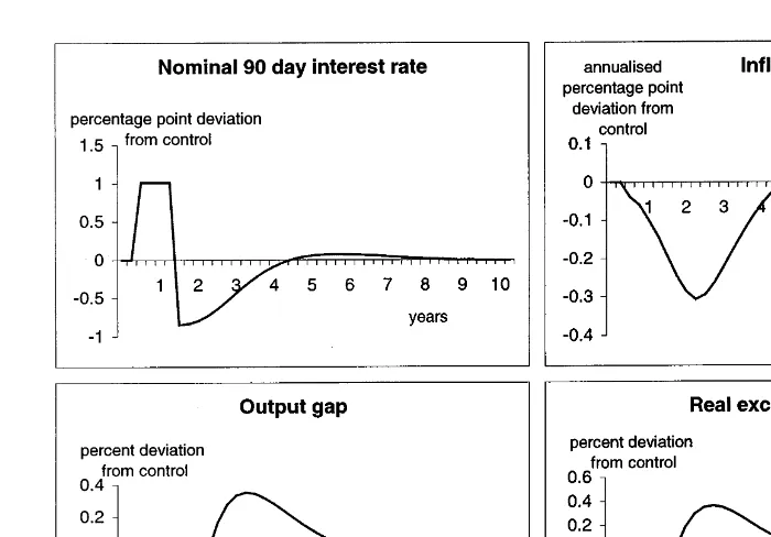
To illustrate some of the properties of the FPS, the model’s dynamic response to a four-quarter one percentage-point increase in the short-term nominal interest rate is graphed in Figure 1.
2See Black et al. (1997) for a more complete description of the FPS model.
3The specification is based on the overlapping-generations framework of Yaari (1965), Blanchard (1985), Weil (1989), and Buiter (1988), but in a discrete time form as in Frenkel and Razin (1992) and Black et al. (1994).
III. Efficient Policy Rules
In this section, three classes of policy rules are examined: inflation-forecast-based (IFB) rules; standard Taylor rules; and inflation-forecast-based rules that include a contempo-raneous output gap term (IFB 1 G). Assuming certainty about potential output, the efficient frontiers are traced out and compared. Consistent with Taylor (1979), the efficient frontier is defined to be the locus of the lowest achievable combinations of inflation and output variability.
Inflation-Forecast-Based (IFB) Rules
5These rules adjust the policy instrument in response to a model-consistent projection of the deviation of inflation from its target rate.6This class of rules can be expressed as
rst5rst *1
O
i51 j
ui~p
t1i
e 2pT! (1)
5Referring to this class of rules as IFB rules is consistent with Haldane and Batinni (1998) and Amano et al. (1999).
6The base-case FPS policy reaction function used in the Bank’s economic projections falls within this class of rules.
Figure 1. Impact of a four-quarter, one percentage-point increase in the short-term nominal interest
where rs is the short-term nominal interest rate,7rs*is its equilibrium equivalent,pTis the policy target, andpte1iis the model-consistent projection of inflation i quarters ahead. The number of leads, j, and the weights,ui, are a calibration choice.
Stochastic simulations of the model and a grid search technique over policy rule coefficients are employed to trace out the efficient frontier.8 To determine the set of efficient policy rules, both the magnitudes of the weights and the targeting horizon are searched over. The targeting horizon is a three-quarter moving window starting from one quarter ahead and extending to 12 quarters ahead (ten different windows in all). The weights,ui, range in value from 0.5 to 20. For each rule considered, the resulting moments
are calculated by averaging the results from 100 draws, each of which is simulated over a 25-year horizon.9The resulting output and CPI inflation variability pairs are graphed in Figure 2.
The measures of variability used are the root mean squared deviation (RMSD) of inflation from its target rate and output from potential output. The asymmetry in the interaction of goods market disequilibrium and inflation in FPS make this the most appropriate measure of variability to use. The consequences of the asymmetric inflation process under stochastic disturbances are that, on average, inflation is above target and output is below its deterministic steady state.10Relative to the standard deviation statistic, the RMSD statistic penalizes policy rules that result in inflation being more above the inflation target and output being further below its deterministic steady-state level.
7In the model code, the policy reaction function is specified in terms of the yield spread. However, substituting the identity that solves for the short-term nominal rate into the policy reaction function yields a policy reaction function as given. Rewriting the reaction function in terms of the short-term nominal interest rate yields identical model properties provided the response coefficients are scaled up by roughly 30 percent.
8The technique for simulating FPS under stochastic disturbances is presented in Drew and Hunt (1998). 9Consistent with the suggestion in Bryant et al. (1993), the first 5 years of simulation results are ignored when computing the summary statistics.
10For a discussion of why the stochastic steady state for output is below the deterministic equilibrium, see Laxton et al. (1994) and Debelle and Laxton (1997).
In Figure 2, the thin line labeledu51 is derived using a weight of one on the projected deviation of inflation from its target rate and varying the forward-looking targeting horizon. At point A, the targeting horizon is one, two and three quarters ahead. Moving from point A to point B, the targeting horizon is extended through to five, six and seven quarters ahead and both inflation and output variability are reduced. As the targeting horizon is extended beyond that point, the variability in output is reduced, but only at the expense of increased variability in inflation.
The thin line labeledu 5 1.4 traces out the results of increasing the weight on the projected inflation gap to 1.4, and varying the targeting horizon. Increasing the weight reduces inflation variability and output variability for rules with targeting windows that start at 5 quarters ahead and beyond. However, for rules with targeting windows that start at horizons of less than five quarters ahead, output variability increases as inflation variability is reduced. As the weights increase, the targeting horizon at which both inflation and output variability can be reduced lengthens. Once the weights reach a level of 6, reduced inflation variability can only be achieved at the expense of increased output variability at all targeting horizons examined. This is the point where the thick line starts to trace out the globally efficient frontier for IFB rules.
Taylor Rules
For convenience, the second class of rules examined is referred to as Taylor rules. However, it should be noted that we use the term Taylor rule to refer to any policy rule where the instrument responds to the contemporaneous deviations of output from potential and year-over-year inflation from target, regardless of the weights.11This class of rule is given by
rst5rs*1u~pt2pT!1d~yt2ypt! (2)
where ytis the log of real output, yptis the log of potential output and IE 7 here anddare
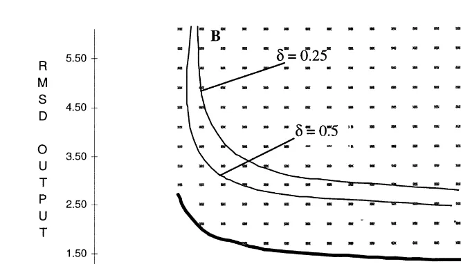
response coefficients. To trace out the efficient frontier under Taylor rules, six weights on the contemporaneous output gap ranging from 0.25 to 10 are examined, in combination with 9 weights on the contemporaneous deviation of inflation from target, ranging from 0.5 to 10.
The output and CPI inflation variability pairs achieved under Taylor rules are graphed in Figure 3. The thin line labeled d 5 0.25 traces out the inflation-output variability trade-off achieved by holding the weight on the output gap fixed at 0.25 and increasing the weight on the inflation gap from 0.5 to 10. Point A has an inflation gap coefficient of 0.5. Moving along the line to point B this weight is increased gradually to 10. Increasing
dto 0.5 shifts the trade-off curve toward the origin, as illustrated by the thin line labeled d50.5. Increasingdup to a value of 6 continues to shift the trade-off curve toward the
origin. No appreciable shifts occur withdvalues larger than 6.
Taylor rules are able to achieve notably lower output variability than IFB rules, but inflation variability is higher regardless of the weight put on the contemporaneous deviation of inflation from target.
Including a Contemporaneous Output Gap in Inflation-Forecast-Based Rules
The final class of rules examined combines aspects of the IFB rules and Taylor rules by including the contemporaneous deviation of output from potential in IFB rules. This class of rules is given by
rst5rst*1
O
i51 jui~p
t1i
e 2pT!1d~y
t2ypt!. (3)
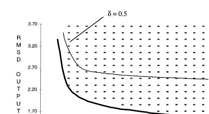
To make the required simulation task manageable, we search over fewer horizons and weights on the forward-looking inflation gap.12Consequently, the frontiers examined here are traced out with slightly fewer observations than for the IFB rules. As with the standard Taylor rules, six alternative values fordare examined ranging from 0.25 to 10.
Comparison of the frontiers traced out in Figure 4 with the IFB frontier in Figure 2, reveals that, for a given level of CPI inflation variability, output variability can be reduced by responding to the contemporaneous output gap in addition to the forward-looking deviation of inflation from target. For example, given inflation variability of 1.0, including the standard Taylor weight of 0.5 on the output gap term reduces output variability from 2.8 to 2.6. The larger is the weight on the output gap, the more output variability can be reduced.13
Comparison of these results to those achieved under Taylor rules illustrates the benefits of policy being forward looking in terms of the deviation of inflation from the target.
12The number of weights on the forward-looking inflation gaps are reduced from 17 to 10 and the number of targeting windows are reduced from 10 to 6.
13This reduction in output variability comes at the cost of increased variability in instruments. Given a RMSD of inflation around 1, increasing the weight on the contemporaneous output gap from 0.5 to 1.5 increases the RMSD in nominal interest rates from 4.6 to only 5.1. However, increasing the weight on output to 6 results in the RMSD of the nominal short-term interest rate increasing to 10.6. This increase in instrument variability is such that the policy rule is not considered when instrument constraints are applied.
Under IFB1G rules, inflation variability in notably reduced relative to that achievable under Taylor rules.
These results differ from those presented in Haldane and Batini (1998), where the inclusion of the contemporaneous output gap did not shift the efficient frontier downwards as it does here. The Haldane and Batini result lead the authors to conclude that IFB rules were “output encompassing.” An obvious potential source of the conflicting result is model specification differences. In addition, a possible explanation is that the search over rule specifications conducted in Haldane and Batini is not quite as general as in the analysis presented in this paper. In Haldane and Battini, the contemporaneous output gap term was included in a rule that had the horizon and weight optimized in the absence of an output gap term. It is possible that a more general search technique would have yielded different results.
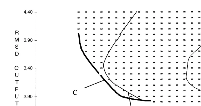
Comparing the Three Classes of Policy Rules
Taylor rules and the inclusion of the contemporaneous output gap in inflation-forecast-based rules yield output and CPI inflation variability combinations not achievable under pure inflation-forecast-based rules. In Figure 5, the achievable frontiers under the three classes of policy rules are compared. Relative to inflation-forecast-based rules, Taylor rules allow for significant improvements in output variability, although they cannot achieve the same inflation variability performance. Including the contemporaneous output gap in inflation-forecast-based rules allows for a similar reduction in output variability, without sacrificing inflation variability performance.
One outcome of achieving reduced output variability by including the contemporane-ous output gap is that instrument variability increases. In many cases this variability would imply that nominal short-term interest rates would often be negative. In similar experi-ments with a simple demand side version of FPS, imposing a non-negativity constraint on
nominal interest rates constrains variability such that their RMSD never exceeds 8.014. The shaded lines in Figure 6 trace out the efficient frontiers that result from considering only the policy rules that result in instrument variability consistent with a non-negativity constraint. This constraint reduces the output variability performance of the rules that include the contemporaneous output gap. The frontier under IFB rules is not materially affected.
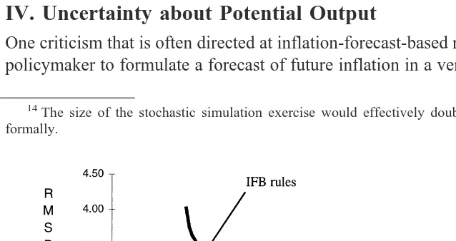
IV. Uncertainty about Potential Output
One criticism that is often directed at inflation-forecast-based rules is that they require the policymaker to formulate a forecast of future inflation in a very uncertain world [see, for
14The size of the stochastic simulation exercise would effectively double if the constraint was imposed formally.
Figure 5. Comparing the efficient frontiers. (RMSD, root mean squared deviation).
example, McCallum and Nelson (1998)]. The policymaker is uncertain about the true structure of the economy, the nature of the disturbances that are likely to occur, and the underlying state of the economy and how it is likely to evolve over the forecast horizon. These are all legitimate concerns that policymakers need to address. In this section, the implications of the policymaker’s uncertainty about one aspect of the state of the economy, its supply capacity, are examined. This is important for IFB rules and rules that rely on the contemporaneous output gap.
Incorporating Uncertainty
To examine the implications of uncertainty about potential output, it is necessary to derive a characterization of what the policymaker’s typical errors about potential output might look like. Methods for estimating the contemporaneous level of potential output used by policymakers often rely on techniques for decomposing real output data into their trend (supply) and cyclical (temporary) components. Examples of these techniques used by policymakers that rely on a variant of the Hodrick and Prescott (1997) filter can be found in Laxton and Tetlow (1992), Butler (1996), Haltmaier (1996), and Conway and Hunt (1997). Harvey and Jaeger (1993) illustrate that techniques based on the Hodrick–Prescott (HP) filter are restricted versions of a more general unobserved-component modeling framework.
The uncertainty about how accurately estimates from unobserved-component models reflect the “true” level of potential output has been shown in Kuttner (1994) to arise from two sources. The first is “filter” or “signal extraction” uncertainty. This arises because even if the parameters of the model are known with certainty, the unobserved state variable still has a noisy link to the data and the estimate must be extracted given the available data set. The second source is “parameter” uncertainty. The parameters of unobserved-component models are estimated using the Kalman (1960) recursion and maximum likelihood techniques. The estimated parameters thus have associated vari-ances. The dimension of uncertainty that is examined here corresponds to filter uncer-tainty. Specifically, we consider the implications that HP filter uncertainty about the monetary authority’s estimate of potential output has on the relative performance of the simple policy rules examined.
A multi-step procedure is used to generate the time-series paths for the errors about potential output arising from HP filter uncertainty. The model is first simulated under the set of seeded disturbances used to generate the 100 draws applied in the experiments under consideration. Policy is characterized as the FPS base-case IFB policy rule and potential output is known with certainty. To extract the proxy for the monetary authority’s typical errors associated with filter uncertainty, the resulting times-series paths for real output from each draw are detrended using the HP filter in two ways. First, the HP filter is run as a true filter through data using only data up to time t to extract the estimate of potential up to and including time t. Next it is run as a smoother using the complete data set up to time T to extract estimates of potential output for all t. The monetary authority’s error about potential output is the difference between the filter estimate and the smoother estimate. As noted in Kuttner (1994), the smoother can be used in this way to extract the level of filter uncertainty associated with an unobserved-component model.
cording to a fixed growth rate in the monetary authority’s forecasting framework. The policy setting solved for within this framework is then sent to the real world along with all the temporary disturbances plus the error on potential output. Given the policy settings, the temporary shocks and the correct level of potential, the model solves for the actual outcome. The process is updated one quarter to date t11, and the monetary authority sets policy again. The monetary authority receives some feedback that it made an error, in that real outcomes and inflation were not as it expected for date t; however, it persists with its view of how potential output evolves. In this set-up, the real world is effectively hit with productivity shocks of which that the monetary authority is always unaware. On average the monetary authority will estimate the level of potential correctly, but over the cycle it makes errors that are persistent and correlated with the evolution of the cycle in each draw.15
It is worth noting that this analysis does not consider whether the HP filter is the “correct” unobserved-component model to be using to estimate potential output. Examples of literature examining this issue are Harvey and Jaeger (1993), Cogely and Nason (1995), and Guay and St–Amant (1996). As noted earlier, the HP filter is a restricted version of a more general unobserved-component model and, consequently, this dimension of the issue should be thought of as parameter uncertainty rather than the filter uncertainty considered here.
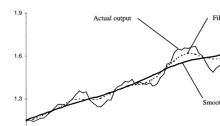
One can argue that this technique provides an effective proxy for the type of errors that a monetary authority might make about the evolution of potential output. In Figure 7, the evolution of real output for one draw under the base-case policy rule is graphed against the proxy for the monetary authority’s current estimate of potential output (filter estimate) and the ex-post estimate of potential output (smoother estimate). When output is expand-ing rapidly, the monetary authority tends to overestimate potential output growth, and
when output growth is weak the monetary authority tends to underestimate potential output growth.
The Implications of Uncertainty
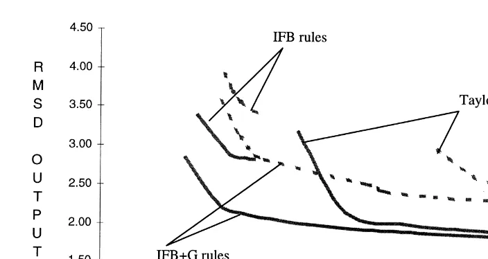
The stochastic experiment in Section III is repeated for all three classes of policy rules under uncertainty about potential output. The relative performance of the three classes of rules is graphed in Figure 8. The solid lines are the efficient frontiers achievable with no
Figure 7. Actual output, filter and smoother estimates of potential output.
Figure 8. The implications of uncertainty for efficient frontiers (RMSD, root mean squared
Rather it reduces the deterioration in inflation variability. For IFB rules, virtually all of the deterioration shows up in an increase in output variability.
The relative shifts in the three classes of efficient rules to some extent reflect the nature of the rules that lie on the efficient frontier. The IFB rules that lie on the frontier are all fairly hawkish, with the magnitude of the weights being 5 or larger on the forward looking inflation gap. However, the efficient frontiers under the other two classes of rules have weights on the inflation gap (forward-looking or contemporaneous) that range from 0.5 to 20. Consequently, some points on these efficient frontiers shift back more in inflation terms than do the IFB rules.
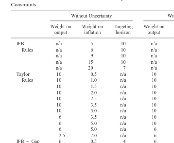
Consideration of the change in the characteristics of efficient rules when uncertainty is introduced illustrates some interesting differences, as shown in Table 1. For the Taylor rules that achieve the very lowest variability in inflation, the weights on inflation and the output gap actually increase under uncertainty about potential output. Efficient Taylor rules that achieve the lowest variability in output undergo no changes in their character-istics. On the other hand, the characteristics of IFB 1 rules that achieve the lowest variability in output do change. For these rules, the forward-looking horizon increases, while the weights remain the same. Under forward-looking inflation targeting rules, the change in characteristics is small and occurs in those that achieve the lowest variability in output. For these rules, the weights on the inflation gap increase slightly under uncertainty. Both the direction and the relatively minor magnitude of the changes in the charac-teristics of efficient rules under this dimension of uncertainty about potential output are rather different from the implications of uncertainty about potential output in Smets (1999) and uncertainty about the natural rate of unemployment in Wieland (1998). In Smets (1999), the observation errors associated with the unobserved-components model considered reduced the degree of activism of optimal Taylor rules. The magnitudes of the optimal coefficients on both the output gap and to a lesser extent the contemporaneous deviation of inflation from target in a Taylor rule declined relative to the case of no uncertainty. In Wieland (1998) uncertainty about the natural rate of unemployment also reduced the optimal degree of policy activism.
reconcile. There are two potential sources for the difference. The first is related to the differences in the nature of the error process considered. The second source compounds the first and is related to the asymmetric inflation process in FPS.
Unlike the estimated Kalman-recursion-observation errors considered in Smets (1999), the HP-filter-uncertainty errors considered here are in general positively correlated with the business cycle. On average over the cycle, the monetary authority underestimates the degree to which output is deviating from potential, and consequently, it forecasts a smaller deviation of inflation from target. Responding less strongly implies inflationary distur-bances get more embedded in expectations. This leads to the second source, the asym-metric inflation process in FPS. Because excess demand leads to more inflationary pressure than an equivalent amount of excess supply leads to deflationary pressure, unwinding inflation shocks requires permanent losses of output. The efficient frontiers presented here are calculated as RMSD from the deterministic steady state and thus they penalize policy rules that lead to larger permanent losses. Up to a point, the less activist the policy rule, the greater will be these losses. It is worth noting that the results obtained here are consistent with those in Isard et al. (1998). Here the authors use a model with a non-linear inflation process similar to that in FPS to examine the implications of uncer-tainty about the natural rate of unemployment. The unceruncer-tainty about the natural rate arises from filter uncertainty associated with an unobserved-component model, and the resulting
Table 1. Characteristics of Some Efficient Policy Rules Without Instrument Variability
errors exhibit similar cyclical variation and serial correlation to the ones considered here. The authors find that increasing the weight on the deviation of inflation from target in a Taylor rule reduces both inflation and output variability under this uncertainty.
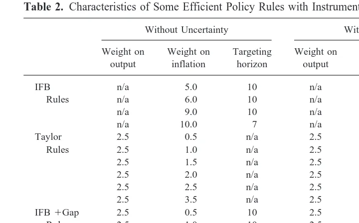
As noted in the previous section, an important consideration is also the variability of nominal interest rates. If the set of rules considered is limited to those with instrument variability consistent with a non-negativity constraint, the efficient frontiers are those traced out in Figure 9. The shaded solid lines trace out the efficient frontiers under certainty and instrument constraints and the shaded dashed lined trace out the implications under uncertainty and instrument constraints. Two points are worth noting that can be inferred from Table 2. The first is that the characteristics of rules that lie on the efficient frontier remain virtually unchanged when uncertainty is introduced for Taylor rules and forward-looking inflation rules that include the contemporaneous output gap. Only the characteristics of IFB rules change under uncertainty with instrument constraints. Under these rules, the effect of uncertainty is still to slightly increase the weights on the inflation gap on those rules that achieve the lowest variability in output. However, the weights do not increase as much as they do when there is no constraint on instrument variability. The second point is that Taylor rules and IFB1G rules are the most affected by the instrument constraint. Again their ability to reduce output variability relative to IFB rules becomes less pronounced. This point is illustrated in Figure 10, which shows the impact of instrument constraints on the efficient frontiers under uncertainty about potential output.
V. Summary and Conclusions
We examine the relative performance of three classes of policy rules using stochastic simulations of the Reserve Bank of New Zealand’s macroeconomic model, FPS. The resulting efficient frontiers achievable under these rules illustrate that Taylor rules can achieve lower output variability than IFB rules. However, to achieve the same inflation variability performance as IFB rules, the inflation gap entering a rule including the
Figure 9. The implications of uncertainty plus instrument constraints (RMSD, root mean squared
contemporaneous output gap needs to be forward looking (IFB1G rule). Consequently, a policy rule containing features of both Taylor rules and inflation-forecast-based rules can achieve outcomes that are unambiguously better than either of the rules can achieve individually. Although reasonable constraints on instrument variability slightly reduce the output variability performance of rules that respond to the contemporaneous output gap, the qualitative story remains the same.
In response to the criticism that uncertainty will reduce the efficacy of IFB rules, the implications of uncertainty about the evolution of potential output are also examined. A
Table 2. Characteristics of Some Efficient Policy Rules with Instrument Variability Constraints
Without Uncertainty With Uncertainty
Figure 10. The implications of instrument constraints under uncertainty (RMSD, root mean
Amano, R., Coletti D., and Macklem T. 1999. Monetary rules when economic behaviour changes. In Monetary Policy Under Uncertainty (B. Hunt and A. Orr, eds.). Wellington, New Zealand: Reserve Bank of New Zealand.
Black, R., Cassino V., Drew A., Hansen, E., Hunt B., Rose, D., and Scott A. 1997. The forecasting and policy system: The core model. Reserve Bank of New Zealand Research Paper No. 43. Wellington.
Black, R., Laxton, D., Rose, D., and Tetlow, R. 1994. The Steady-State Model: SSQPM. The Bank of Canada’s New Quarterly Projection Model, Part 1. Technical Report No. 72. Ottawa: Bank of Canada.
Black, R., Macklem, T., and Rose, D. 1998. On policy rules for price stability. In Price Stability, Inflation Targets and Monetary Policy. Ottawa: Bank of Canada Conference Volume. Blanchard, O. J. 1985. Debt, deficits and finite lives. Journal of Political Economy 93:223–247. Brainard, W. 1967. Uncertainty and the effectiveness of policy. American Economic Review
57:411–425.
Bryant, R., Hooper, P., and Mann, C. 1993. Evaluating Policy Regimes: New Research in Empirical Macroeconomics. Washington, DC: The Brooking Institution.
Buiter, W. H. 1988. Death, birth, productivity growth and debt neutrality. The Economic Journal 98(June):279–293.
Butler, L. 1996. A Semi-Structural Approach to Estimating Potential Output: Combining Economic Theory with a Time-Series Filter. Technical Report No 76. Ottawa: Bank of Canada.
Clarida R., Gali, J., and Gertler, M. 1997. Monetary Policy Rules in Practice: Some International Evidence. NBER Working Paper No. 6254.
Cogely, T., and Nason, J. 1995. Effects of the Hodrick–Prescott filter on trend and difference stationary time series: Implications for business-cycle research. Journal of Economic Dynamics and Control 19:253–278.
Conway, P., and Hunt, B. 1997. Estimating potential output: a semi structural approach. Reserve Bank of New Zealand Discussion Paper G97/9, Wellington.
Debelle, G., and Laxton, D. 1997. Is the Phillips curve really a curve? Some evidence for Canada, the United Kingdom, and the United States. International Monetary Fund Staff Papers 44(2): 249–282.
Drew, A. and Hunt, B. 1998. The Forecasting and Policy System: Stochastic Simulations of the Core Model. Discussion Paper G98/6. Reserve Bank of New Zealand, Wellington.
Fuhrer, J. 1994. Optimal Monetary Policy in a Model of Overlapping Price Contracts. Federal Reserve Bank of Boston. Working Paper No. 94-2 (July).
Guay, A. and St-Amant, P. 1996. Do Mechanical Filters Provide a Good Approximation of Business Cycles? Bank of Canada Technical Report No 78, Bank of Canada, Ottawa.
Haldane, A., and Batini, N. 1998. Forward-looking rules for monetary policy. In Monetary Policy Rules (J.B. Taylor, ed.). Chicago: University Press for NBER.
Haltmaier, J. 1996. Inflation adjusted potential output. International Finance Discussion Papers, No. 561, Board of Governors of the Federal Reserve System.
Harvey, A., and Jaeger, A. 1993. Detrending, stylized facts and the business cycle. Journal of Applied Econometrics 8:231–247.
Hodrick, R., and Prescott, E. 1997. Post-war U.S. business cycles: An empirical investigation. Journal of Money Credit and Banking 29:1–16.
Isard, P., Laxton, D., and Eliasson, A. 1998. Inflation targeting with NAIRU uncertainty and endogenous policy credibility. Paper presented at the Fourth Conference on Computational Economics, Cambridge, United Kingdom.
Kalman, R. 1960. A new approach to linear filtering and prediction problems. Journal of Basic Engineering 82:35–45.
Kuttner, K. 1994. Estimating potential output as a latent variable. Journal of Business and Economic Statistics 12:361–368.
Laxton, D., and Tetlow, R. 1992. A simple multivariate filter for the estimation of potential output. Technical Report No. 59. Ottawa: Bank of Canada.
Laxton, D., Rose, D., and Tetlow, R. 1994. Monetary policy, uncertainty and the presumption of linearity. Technical Report No. 63. Ottawa: Bank of Canada.
Levin, A., Wieland, V., and Williams, J. 1998. Robustness of simple monetary policy rules under model uncertainty. NBER Working Paper No. 6570.
McCallum, B., and Nelson, E. 1998. Performance of operational monetary policy rules in an estimated semi-classical structural model. In Monetary Policy Rules (J. B. Taylor, ed.). Chicago: University Press for NBER.
Rudebusch, G. 1998. Is the Fed too timid? Monetary policy in an uncertain world. Paper presented at the NBER conference Formulation of Monetary Policy, Cambridge, Massachusetts. Rudebusch, G., and Svensson, L. 1998. Policy rules for inflation targeting. In Monetary Policy Rules
(J. B. Taylor, ed.) . Chicago: University Press for NBER.
Smets, F. 1999. Output gap uncertainty: Does it matter for the Taylor rule? Monetary Policy Under Uncertainty (B. Hunt and A. Orr, eds.). Wellington, New Zealand: Reserve Bank of New Zealand.
Taylor, J. 1979. Estimation and control of a macroeconomic model with rational expectations. Econometrica 47:1267–1286.
Taylor, J. 1993. Discretion versus policy rules in practice. Carnegie-Rochester Series on Public Policy 39:195–214.
Tinsley, P. A. 1993. Fitting both data and theories: Polynomial adjustment costs and error-correction decision rules. FRB FEDS Working Paper 93-21.
Weil, P. 1989. Overlapping families of infinitely-lived agents. Journal of Public Economics 38:183–198.
Wieland, V. 1998. Monetary Policy and Uncertainty about the Natural Unemployment Rate. Paper presented at the NBER conference on Formulation of Monetary Policy.