CIVIL
CIVIL
ENGINEERING
FORMULAS
Tyler G. Hicks,
P.E.
International Engineering Associates Member: American Society of Mechanical Engineers
United States Naval Institute
McGRAW-HILL
New York Chicago San Francisco Lisbon London Madrid Mexico City Milan New Delhi San Juan
Copyright © 2002 by The McGraw-Hill Companies. All rights reserved. Manufactured in the United States of America. Except as permitted under the United States Copyright Act of 1976, no part of this publication may be reproduced or distributed in any form or by any means, or stored in a data-base or retrieval system, without the prior written permission of the publisher.
0-07-139542-3
The material in this eBook also appears in the print version of this title: 0-07-135612-3. All trademarks are trademarks of their respective owners. Rather than put a trademark symbol after every occurrence of a trademarked name, we use names in an editorial fashion only, and to the benefit of the trademark owner, with no intention of infringement of the trademark. Where such designations appear in this book, they have been printed with initial caps.
McGraw-Hill eBooks are available at special quantity discounts to use as premiums and sales pro-motions, or for use in corporate training programs. For more information, please contact George Hoare, Special Sales, at [email protected] or (212) 904-4069.
TERMS OF USE
This is a copyrighted work and The McGraw-Hill Companies, Inc. (“McGraw-Hill”) and its licen-sors reserve all rights in and to the work. Use of this work is subject to these terms. Except as per-mitted under the Copyright Act of 1976 and the right to store and retrieve one copy of the work, you may not decompile, disassemble, reverse engineer, reproduce, modify, create derivative works based upon, transmit, distribute, disseminate, sell, publish or sublicense the work or any part of it without McGraw-Hill’s prior consent. You may use the work for your own noncommercial and personal use; any other use of the work is strictly prohibited. Your right to use the work may be terminated if you fail to comply with these terms.
THE WORK IS PROVIDED “AS IS”. McGRAW-HILL AND ITS LICENSORS MAKE NO GUARANTEES OR WARRANTIES AS TO THE ACCURACY, ADEQUACY OR COM-PLETENESS OF OR RESULTS TO BE OBTAINED FROM USING THE WORK, INCLUDING ANY INFORMATION THAT CAN BE ACCESSED THROUGH THE WORK VIA HYPER-LINK OR OTHERWISE, AND EXPRESSLY DISCLAIM ANY WARRANTY, EXPRESS OR IMPLIED, INCLUDING BUT NOT LIMITED TO IMPLIED WARRANTIES OF MER-CHANTABILITY OR FITNESS FOR A PARTICULAR PURPOSE. McGraw-Hill and its licen-sors do not warrant or guarantee that the functions contained in the work will meet your require-ments or that its operation will be uninterrupted or error free. Neither McGraw-Hill nor its licen-sors shall be liable to you or anyone else for any inaccuracy, error or omission, regardless of cause, in the work or for any damages resulting therefrom. McGraw-Hill has no responsibility for the content of any information accessed through the work. Under no circumstances shall McGraw-Hill and/or its licensors be liable for any indirect, incidental, special, punitive, consequential or similar damages that result from the use of or inability to use the work, even if any of them has been advised of the possibility of such damages. This limitation of liability shall apply to any claim or cause whatsoever whether such claim or cause arises in contract, tort or otherwise. DOI: 10.1036/0071395423
abc
CONTENTS
Preface xiii
Acknowledgments xv
How to Use This Book xvii
Chapter 1. Conversion Factors for Civil
Engineering Practice 1
Chapter 2. Beam Formulas 15
Continuous Beams / 16
Ultimate Strength of Continuous Beams / 53 Beams of Uniform Strength / 63
Safe Loads for Beams of Various Types / 64 Rolling and Moving Loads / 79
Curved Beams / 82
Elastic Lateral Buckling of Beams / 88 Combined Axial and Bending Loads / 92 Unsymmetrical Bending / 93
Eccentric Loading / 94
Natural Circular Frequencies and Natural Periods of Vibration of Prismatic Beams / 96
Chapter 3. Column Formulas 99
General Considerations / 100 Short Columns / 102
Eccentric Loads on Columns / 102 Column Base Plate Design / 111
American Institute of Steel Construction Allowable-Stress Design Approach / 113
Composite Columns / 115
Elastic Flexural Buckling of Columns / 118
Allowable Design Loads for Aluminum Columns / 121 Ultimate-Strength Design of Concrete Columns / 124
Chapter 4. Piles and Piling Formulas 131
Allowable Loads on Piles / 132 Laterally Loaded Vertical Piles / 133 Toe Capacity Load / 134
Groups of Piles / 136
Foundation-Stability Analysis / 139 Axial-Load Capacity of Single Piles / 143 Shaft Settlement / 144
Shaft Resistance to Cohesionless Soil / 145
Chapter 5. Concrete Formulas 147
Reinforced Concrete / 148
Water/Cementitious Materials Ratio / 148 Job Mix Concrete Volume / 149 Modulus of Elasticity of Concrete / 150 Tensile Strength of Concrete / 151 Reinforcing Steel / 151
Continuous Beams and One-Way Slabs / 151
Design Methods for Beams, Columns, and Other Members / 153 Properties in the Hardened State / 167
Compression at Angle to Grain / 220
Recommendations of the Forest Products Laboratory / 221 Compression on Oblique Plane / 223
Adjustments Factors for Design Values / 224 Fasteners for Wood / 233
Adjustment of Design Values for Connections with Fasteners / 236
Roof Slope to Prevent Ponding / 238 Bending and Axial Tension / 239 Bending and Axial Compression / 240
Chapter 7. Surveying Formulas 243
Units of Measurement / 244 Theory of Errors / 245
Measurement of Distance with Tapes / 247 Vertical Control / 253
Stadia Surveying / 253 Photogrammetry / 255
Chapter 8. Soil and Earthwork Formulas 257
Physical Properties of Soils / 258 Index Parameters for Soils / 259
Relationship of Weights and Volumes in Soils / 261 Internal Friction and Cohesion / 263
Vertical Pressures in Soils / 264
Lateral Pressures in Soils, Forces on Retaining Walls / 265 Lateral Pressure of Cohesionless Soils / 266
Lateral Pressure of Cohesive Soils / 267 Water Pressure / 268
Lateral Pressure from Surcharge / 268 Stability of Slopes / 269
Bearing Capacity of Soils / 270 Settlement under Foundations / 271 Soil Compaction Tests / 272
Compaction Equipment / 275 Formulas for Earthmoving / 276 Scraper Production / 278 Vibration Control in Blasting / 280
Chapter 9. Building and Structures Formulas 283
Load-and-Resistance Factor Design for Shear in Buildings / 284 Allowable-Stress Design for Building Columns / 285
Load-and-Resistance Factor Design for Building Columns / 287 Allowable-Stress Design for Building Beams / 287
Load-and-Resistance Factor Design for Building Beams / 290 Allowable-Stress Design for Shear in Buildings / 295 Stresses in Thin Shells / 297
Bearing Plates / 298 Column Base Plates / 300 Bearing on Milled Surfaces / 301 Plate Girders in Buildings / 302
Load Distribution to Bents and Shear Walls / 304
Combined Axial Compression or Tension and Bending / 306 Webs under Concentrated Loads / 308
Design of Stiffeners under Loads / 311 Fasteners for Buildings / 312 Composite Construction / 313
Number of Connectors Required for Building Construction / 316 Ponding Considerations in Buildings / 318
Chapter 10. Bridge and Suspension-Cable
Formulas 321
Shear Strength Design for Bridges / 322
Allowable-Stress Design for Bridge Columns / 323
Load-and-Resistance Factor Design for Bridge Columns / 324 Allowable-Stress Design for Bridge Beams / 325
Stiffeners on Bridge Girders / 327 Hybrid Bridge Girders / 329
Load-Factor Design for Bridge Beams / 330 Bearing on Milled Surfaces / 332
Bridge Fasteners / 333
Composite Construction in Highway Bridges / 333 Number of Connectors in Bridges / 337
Allowable-Stress Design for Shear in Bridges / 339 Maximum Width/Thickness Ratios for Compression
Elements for Highway Bridges / 341 Suspension Cables / 341
General Relations for Suspension Cables / 345 Cable Systems / 353
Chapter 11. Highway and Road Formulas 355
Circular Curves / 356 Parabolic Curves / 359
Highway Curves and Driver Safety / 361 Highway Alignments / 362
Structural Numbers for Flexible Pavements / 365 Transition (Spiral) Curves / 370
Designing Highway Culverts / 371
American Iron and Steel Institute (AISI) Design Procedure / 374
Chapter 12. Hydraulics and Waterworks
Formulas 381
Capillary Action / 382 Viscosity / 386
Pressure on Submerged Curved Surfaces / 387 Fundamentals of Fluid Flow / 388
Similitude for Physical Models / 392 Fluid Flow in Pipes / 395
Pressure (Head) Changes Caused by Pipe Size Change / 403 Flow through Orifices / 406
Fluid Jets / 409
Orifice Discharge into Diverging Conical Tubes / 410 Water Hammer / 412
Pipe Stresses Perpendicular to the Longitudinal Axis / 412 Temperature Expansion of Pipe / 414
Forces Due to Pipe Bends / 414 Culverts / 417
Open-Channel Flow / 420
Manning’s Equation for Open Channels / 424 Hydraulic Jump / 425
Nonuniform Flow in Open Channels / 429 Weirs / 436
Flow Over Weirs / 438
Prediction of Sediment-Delivery Rate / 440 Evaporation and Transpiration / 442 Method for Determining Runoff for Minor
Hydraulic Structures / 443 Computing Rainfall Intensity / 443 Groundwater / 446
Water Flow for Firefighting / 446 Flow from Wells / 447
Economical Sizing of Distribution Piping / 448 Venturi Meter Flow Computation / 448 Hydroelectric Power Generation / 449
Index 451
PREFACE
This handy book presents more than 2000 needed formulas for civil engineers to help them in the design office, in the field, and on a variety of construction jobs, anywhere in the world. These formulas are also useful to design drafters, structural engineers, bridge engineers, foundation builders, field engineers, professional-engineer license examination candidates, concrete specialists, timber-structure builders, and students in a variety of civil engineering pursuits.
The book presents formulas needed in 12 different spe-cialized branches of civil engineering—beams and girders, columns, piles and piling, concrete structures, timber engi-neering, surveying, soils and earthwork, building struc-tures, bridges, suspension cables, highways and roads, and hydraulics and open-channel flow. Key formulas are pre-sented for each of these topics. Each formula is explained so the engineer, drafter, or designer knows how, where, and when to use the formula in professional work. Formula units are given in both the United States Customary System (USCS) and System International (SI). Hence, the text is usable throughout the world. To assist the civil engineer using this material in worldwide engineering practice, a com-prehensive tabulation of conversion factors is presented in Chapter 1.
In assembling this collection of formulas, the author was guided by experts who recommended the areas of
greatest need for a handy book of practical and applied civil engineering formulas.
Sources for the formulas presented here include the var-ious regulatory and industry groups in the field of civil engi-neering, authors of recognized books on important topics in the field, drafters, researchers in the field of civil engineer-ing, and a number of design engineers who work daily in the field of civil engineering. These sources are cited in the Acknowledgments.
When using any of the formulas in this book that may come from an industry or regulatory code, the user is cautioned to consult the latest version of the code. Formulas may be changed from one edition of a code to the next. In a work of this magnitude it is difficult to include the latest formulas from the numerous constant-ly changing codes. Hence, the formulas given here are those current at the time of publication of this book.
In a work this large it is possible that errors may occur. Hence, the author will be grateful to any user of the book who detects an error and calls it to the author’s attention. Just write the author in care of the publisher. The error will be corrected in the next printing.
In addition, if a user believes that one or more important formulas have been left out, the author will be happy to consider them for inclusion in the next edition of the book. Again, just write him in care of the publisher.
Tyler G. Hicks, P.E.
ACKNOWLEDGMENTS
Many engineers, professional societies, industry associa-tions, and governmental agencies helped the author find and assemble the thousands of formulas presented in this book. Hence, the author wishes to acknowledge this help and assistance.
The author’s principal helper, advisor, and contributor was the late Frederick S. Merritt, P.E., Consulting Engineer. For many years Fred and the author were editors on com-panion magazines at The McGraw-Hill Companies. Fred was an editor on Engineering-News Record, whereas the
author was an editor on Power magazine. Both lived on
Long Island and traveled on the same railroad to and from New York City, spending many hours together discussing engineering, publishing, and book authorship.
When the author was approached by the publisher to pre-pare this book, he turned to Fred Merritt for advice and help. Fred delivered, preparing many of the formulas in this book and giving the author access to many more in Fred’s exten-sive files and published materials. The author is most grate-ful to Fred for his extensive help, advice, and guidance.
Further, the author thanks the many engineering soci-eties, industry associations, and governmental agencies whose work is referred to in this publication. These organizations provide the framework for safe design of numerous struc-tures of many different types.
The author also thanks Larry Hager, Senior Editor, Pro-fessional Group, The McGraw-Hill Companies, for his excellent guidance and patience during the long preparation of the manuscript for this book. Finally, the author thanks his wife, Mary Shanley Hicks, a publishing professional, who always most willingly offered help and advice when needed.
Specific publications consulted during the preparation of this text include: American Association of State Highway and Transportation Officials (AASHTO) “Standard Specifi-cations for Highway Bridges”; American Concrete Institute (ACI) “Building Code Requirements for Reinforced Con-crete”; American Institute of Steel Construction (AISC) “Manual of Steel Construction,” “Code of Standard Prac-tice,” and “Load and Resistance Factor Design Specifica-tions for Structural Steel Buildings”; American Railway Engineering Association (AREA) “Manual for Railway Engineering”; American Society of Civil Engineers (ASCE) “Ground Water Management”; American Water Works Association (AWWA) “Water Quality and Treat-ment.” In addition, the author consulted several hundred civil engineering reference and textbooks dealing with the topics in the current book. The author is grateful to the writers of all the publications cited here for the insight they gave him to civil engineering formulas. A number of these works are also cited in the text of this book.
HOW TO USE
THIS BOOK
The formulas presented in this book are intended for use by civil engineers in every aspect of their professional work— design, evaluation, construction, repair, etc.
To find a suitable formula for the situation you face, start by consulting the index. Every effort has been made to present a comprehensive listing of all formulas in the book. Once you find the formula you seek, read any accompa-nying text giving background information about the formula. Then when you understand the formula and its applications, insert the numerical values for the variables in the formula. Solve the formula and use the results for the task at hand.
Where a formula may come from a regulatory code, or where a code exists for the particular work being done, be certain to check the latest edition of the appli-cable code to see that the given formula agrees with the code formula. If it does not agree, be certain to use the latest code formula available. Remember, as a design engineer you are responsible for the structures you plan, design, and build. Using the latest edition of any govern-ing code is the only sensible way to produce a safe and dependable design that you will be proud to be associ-ated with. Further, you will sleep more peacefully!
CHAPTER 1
CONVERSION
FACTORS FOR
CIVIL
ENGINEERING
PRACTICE
Civil engineers throughout the world accept both the
United States Customary System (USCS) and the System International (SI) units of measure for both applied and
theoretical calculations. However, the SI units are much more widely used than those of the USCS. Hence, both the USCS and the SI units are presented for essentially every formula in this book. Thus, the user of the book can apply the formulas with confidence anywhere in the world.
To permit even wider use of this text, this chapter con-tains the conversion factors needed to switch from one sys-tem to the other. For engineers unfamiliar with either system of units, the author suggests the following steps for becoming acquainted with the unknown system:
1. Prepare a list of measurementscommonly used in your
daily work.
2. Insert, opposite each known unit,the unit from the other
system. Table 1.1 shows such a list of USCS units with corresponding SI units and symbols prepared by a civil engineer who normally uses the USCS. The SI units shown in Table 1.1 were obtained from Table 1.3 by the engineer.
3. Find, from a table of conversion factors,such as Table 1.3,
the value used to convert from USCS to SI units. Insert each appropriate value in Table 1.2 from Table 1.3.
4. Apply the conversion valueswherever necessary for the
formulas in this book.
5. Recognize—here and now—that the most difficult
aspect of becoming familiar with a new system of meas-urement is becoming comfortable with the names and magnitudes of the units. Numerical conversion is simple, once you have set up your own conversion table.
Be careful, when using formulas containing a numerical constant, to convert the constant to that for the system you are using. You can, however, use the formula for the USCS units (when the formula is given in those units) and then convert the final result to the SI equivalent using Table 1.3. For the few formulas given in SI units, the reverse proce-dure should be used.
CONVERSION FACTORS 3
TABLE 1.1 Commonly Used USCS and SI Units†
Conversion factor (multiply USCS unit
by this factor to
USCS unit SI unit SI symbol obtain SI unit)
square foot square meter m2 0.0929
cubic foot cubic meter m3 0.2831
pound per
square inch kilopascal kPa 6.894
pound force newton Nu 4.448
foot pound
torque newton meter Nm 1.356
kip foot kilonewton meter kNm 1.355
gallon per
minute liter per second L/s 0.06309
kip per square
inch megapascal MPa 6.89
4 CHAPTER ONE
TABLE 1.2 Typical Conversion Table†
To convert from To Multiply by‡
square foot square meter 9.290304 E02 foot per second meter per second
squared squared 3.048 E01
cubic foot cubic meter 2.831685 E02 pound per cubic kilogram per cubic
inch meter 2.767990 E04
gallon per minute liter per second 6.309 E02 pound per square
inch kilopascal 6.894757
pound force newton 4.448222
kip per square foot pascal 4.788026 E04 acre foot per day cubic meter per E02
second 1.427641
acre square meter 4.046873 E03
cubic foot per cubic meter per
second second 2.831685 E02
†This table contains only selected values. See the U.S. Department of the
Interior Metric Manual, or National Bureau of Standards,The International System of Units(SI), both available from the U.S. Government Printing Office (GPO), for far more comprehensive listings of conversion factors.
‡The E indicates an exponent, as in scientific notation, followed by a positive
or negative number, representing the power of 10 by which the given version factor is to be multiplied before use. Thus, for the square foot con-version factor, 9.2903041/1000.09290304, the factor to be used to convert square feet to square meters. For a positive exponent, as in convert-ing acres to square meters, multiply by 4.04687310004046.8.
Where a conversion factor cannot be found, simply use the dimensional substitution. Thus, to convert pounds per cubic inch to kilograms per cubic meter, find 1 lb0.4535924 kg and 1 in30.00001638706 m3. Then,
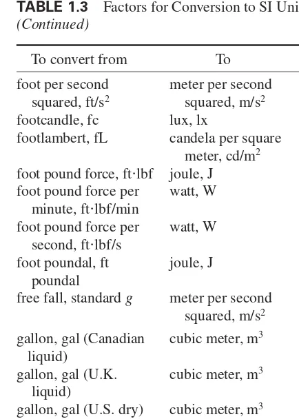
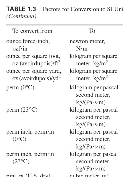
TABLE 1.3 Factors for Conversion to SI Units of Measurement
To convert from To Multiply by
acre foot, acre ft cubic meter, m3 1.233489 E03
acre square meter, m2 4.046873 E03
angstrom, Å meter, m 1.000000* E10
atmosphere, atm pascal, Pa 1.013250* E05
(standard)
atmosphere, atm pascal, Pa 9.806650* E04
(technical 1 kgf/cm2)
bar pascal, Pa 1.000000* E05
barrel (for petroleum, cubic meter, m2 1.589873 E01
42 gal)
board foot, board ft cubic meter, m3 2.359737 E03
British thermal unit, joule, J 1.05587 E03 Btu, (mean)
British thermal unit, watt per meter 1.442279 E01 Btu (International kelvin, W/(mK)
Table)in/(h)(ft2)
(°F) (k, thermal conductivity)
British thermal unit, watt, W 2.930711 E01 Btu (International
Table)/h
British thermal unit, watt per square 5.678263 E00 Btu (International meter kelvin,
Table)/(h)(ft2)(°F) W/(m2K)
(C, thermal conductance)
British thermal unit, joule per kilogram, 2.326000* E03
Btu (International J/kg Table)/lb
TABLE 1.3 Factors for Conversion to SI Units of Measurement (Continued)
To convert from To Multiply by
British thermal unit, joule per kilogram 4.186800* E03
Btu (International kelvin, J/(kgK) Table)/(lb)(°F)
(c, heat capacity)
British thermal unit, joule per cubic 3.725895 E04 cubic foot, Btu meter, J/m3
(International Table)/ft3
bushel (U.S.) cubic meter, m3 3.523907 E02
calorie (mean) joule, J 4.19002 E00 candela per square candela per square 1.550003 E03
inch, cd/in2 meter, cd/m2
centimeter, cm, of pascal, Pa 1.33322 E03 mercury (0°C)
centimeter, cm, of pascal, Pa 9.80638 E01 water (4°C)
chain meter, m 2.011684 E01
circular mil square meter, m2 5.067075 E10
day second, s 8.640000* E04
day (sidereal) second, s 8.616409 E04 degree (angle) radian, rad 1.745329 E02 degree Celsius kelvin, K TKtC273.15 degree Fahrenheit degree Celsius, °C tC(tF32)/1.8 degree Fahrenheit kelvin, K TK(tF459.67)/1.8 degree Rankine kelvin, K TKTR/1.8 (°F)(h)(ft2)/Btu kelvin square 1.761102 E01
(International meter per watt, Table) (R, thermal Km2/W
resistance)
TABLE 1.3 Factors for Conversion to SI Units of Measurement (Continued)
To convert from To Multiply by
(°F)(h)(ft2)/(Btu kelvin meter per 6.933471 E00
(International watt, Km/W Table)in) (thermal
resistivity)
dyne, dyn newton, N 1.000000† E05
fathom meter, m 1.828804 E00
foot, ft meter, m 3.048000† E01
foot, ft (U.S. survey) meter, m 3.048006 E01 foot, ft, of water pascal, Pa 2.98898 E03
(39.2°F) (pressure)
square foot, ft2 square meter, m2 9.290304† E02
square foot per hour, square meter per 2.580640† E05
ft2/h (thermal second, m2/s
diffusivity)
square foot per square meter per 9.290304† E02
second, ft2/s second, m2/s
cubic foot, ft3(volume cubic meter, m3 2.831685 E02
or section modulus)
cubic foot per minute, cubic meter per 4.719474 E04 ft3/min second, m3/s
cubic foot per second, cubic meter per 2.831685 E02 ft3/s second, m3/s
foot to the fourth meter to the fourth 8.630975 E03 power, ft4(area power, m4
moment of inertia)
foot per minute, meter per second, 5.080000† E03
ft/min m/s
foot per second, meter per second, 3.048000† E01
ft/s m/s
TABLE 1.3 Factors for Conversion to SI Units of Measurement (Continued)
To convert from To Multiply by
foot per second meter per second 3.048000† E01
squared, ft/s2 squared, m/s2
footcandle, fc lux, lx 1.076391 E01 footlambert, fL candela per square 3.426259 E00
meter, cd/m2
foot pound force, ftlbf joule, J 1.355818 E00 foot pound force per watt, W 2.259697 E02
minute, ftlbf/min
foot pound force per watt, W 1.355818 E00 second, ftlbf/s
foot poundal, ft joule, J 4.214011 E02 poundal
free fall, standard g meter per second 9.806650† E00 squared, m/s2
gallon, gal (Canadian cubic meter, m3 4.546090 E03
liquid)
gallon, gal (U.K. cubic meter, m3 4.546092 E03
liquid)
gallon, gal (U.S. dry) cubic meter, m3 4.404884 E03
gallon, gal (U.S. cubic meter, m3 3.785412 E03
liquid)
gallon, gal (U.S. cubic meter per 4.381264 E08 liquid) per day second, m3/s
gallon, gal (U.S. cubic meter per 6.309020 E05 liquid) per minute second, m3/s
grad degree (angular) 9.000000† E01
grad radian, rad 1.570796 E02
grain, gr kilogram, kg 6.479891† E05
gram, g kilogram, kg 1.000000† E03
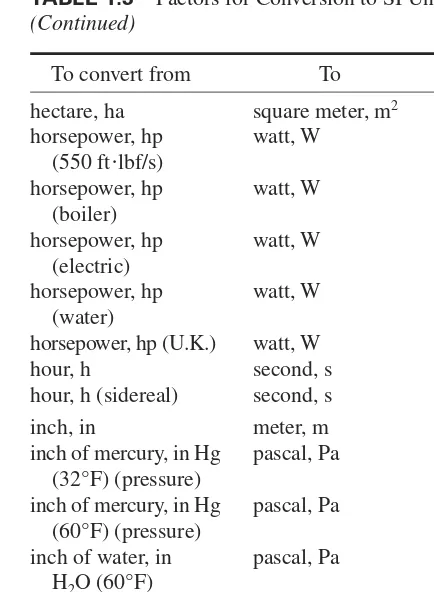
TABLE 1.3 Factors for Conversion to SI Units of Measurement (Continued)
To convert from To Multiply by
hectare, ha square meter, m2 1.000000† E04
horsepower, hp watt, W 7.456999 E02 (550 ftlbf/s)
horsepower, hp watt, W 9.80950 E03 (boiler)
horsepower, hp watt, W 7.460000† E02
(electric)
horsepower, hp watt, W 7.46043† E02
(water)
horsepower, hp (U.K.) watt, W 7.4570 E02
hour, h second, s 3.600000† E03
hour, h (sidereal) second, s 3.590170 E03
inch, in meter, m 2.540000† E02
inch of mercury, in Hg pascal, Pa 3.38638 E03 (32°F) (pressure)
inch of mercury, in Hg pascal, Pa 3.37685 E03 (60°F) (pressure)
inch to the fourth meter to the fourth 4.162314 E07 power, in4(area power, m4
moment of inertia)
inch per second, in/s meter per second, 2.540000† E02
m/s
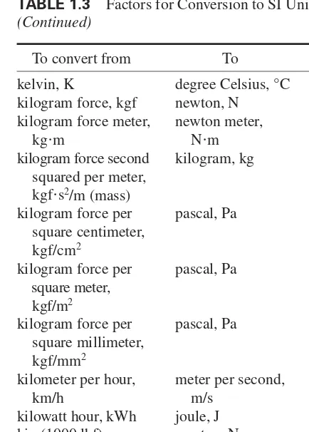
TABLE 1.3 Factors for Conversion to SI Units of Measurement (Continued)
To convert from To Multiply by
kelvin, K degree Celsius, °C tCTK273.15 kilogram force, kgf newton, N 9.806650† E00
kilogram force meter, newton meter, 9.806650† E00
kgm Nm
kilogram force second kilogram, kg 9.806650† E00
squared per meter, kgfs2/m (mass)
kilogram force per pascal, Pa 9.806650† E04
square centimeter, kgf/cm2
kilogram force per pascal, Pa 9.806650† E00
square meter, kgf/m2
kilogram force per pascal, Pa 9.806650† E06
square millimeter, kgf/mm2
kilometer per hour, meter per second, 2.777778 E01
km/h m/s
kilowatt hour, kWh joule, J 3.600000† E06
kip (1000 lbf) newton, N 4.448222 E03 kipper square inch, pascal, Pa 6.894757 E06
kip/in2ksi
knot, kn (international) meter per second, 5.144444 E01 m/s
lambert, L candela per square 3.183099 E03 meter, cd/m
liter cubic meter, m3 1.000000† E03
maxwell weber, Wb 1.000000† E08
mho siemens, S 1.000000† E00
CONVERSION FACTORS 11
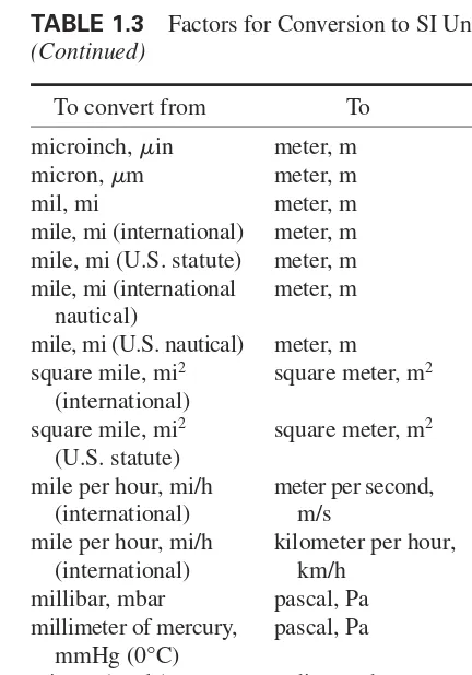
TABLE 1.3 Factors for Conversion to SI Units of Measurement (Continued)
To convert from To Multiply by
microinch,in meter, m 2.540000† E08
micron,m meter, m 1.000000† E06
mil, mi meter, m 2.540000† E05
mile, mi (international) meter, m 1.609344† E03
mile, mi (U.S. statute) meter, m 1.609347 E03 mile, mi (international meter, m 1.852000† E03
nautical)
mile, mi (U.S. nautical) meter, m 1.852000† E03
square mile, mi2 square meter, m2 2.589988 E06
(international)
square mile, mi2 square meter, m2 2.589998 E06
(U.S. statute)
mile per hour, mi/h meter per second, 4.470400† E01
(international) m/s
mile per hour, mi/h kilometer per hour, 1.609344† E00
(international) km/h
millibar, mbar pascal, Pa 1.000000† E02
millimeter of mercury, pascal, Pa 1.33322 E02 mmHg (0°C)
minute (angle) radian, rad 2.908882 E04 minute, min second, s 6.000000† E01
minute (sidereal) second, s 5.983617 E01 ounce, oz kilogram, kg 2.834952 E02
(avoirdupois)
ounce, oz (troy or kilogram, kg 3.110348 E02 apothecary)
ounce, oz (U.K. fluid) cubic meter, m3 2.841307 E05
ounce, oz (U.S. fluid) cubic meter, m3 2.957353 E05
TABLE 1.3 Factors for Conversion to SI Units of Measurement (Continued)
To convert from To Multiply by
ounce forceinch, newton meter, 7.061552 E03
ozfin Nm
ounce per square foot, kilogram per square 3.051517 E01 oz (avoirdupois)/ft2 meter, kg/m2
ounce per square yard, kilogram per square 3.390575 E02 oz (avoirdupois)/yd2 meter, kg/m2
perm (0°C) kilogram per pascal 5.72135 E11 second meter,
kg/(Pasm)
perm (23°C) kilogram per pascal 5.74525 E11 second meter,
kg/(Pasm)
perm inch, permin kilogram per pascal 1.45322 E12
(0°C) second meter,
kg/(Pasm)
perm inch, permin kilogram per pascal 1.45929 E12
(23°C) second meter,
kg/(Pasm)
pint, pt (U.S. dry) cubic meter, m3 5.506105 E04
pint, pt (U.S. liquid) cubic meter, m3 4.731765 E04
poise, p (absolute pascal second, 1.000000† E01
viscosity) Pas
pound, lb kilogram, kg 4.535924 E01 (avoirdupois)
pound, lb (troy or kilogram, kg 3.732417 E01 apothecary)
pound square inch, kilogram square 2.926397 E04 lbin2(moment of meter, kgm2
inertia)
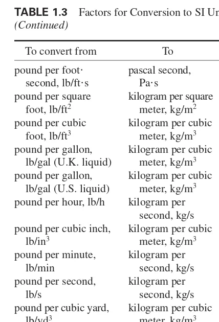
TABLE 1.3 Factors for Conversion to SI Units of Measurement (Continued)
To convert from To Multiply by
pound per foot pascal second, 1.488164 E00 second, lb/fts Pas
pound per square kilogram per square 4.882428 E00 foot, lb/ft2 meter, kg/m2
pound per cubic kilogram per cubic 1.601846 E01 foot, lb/ft3 meter, kg/m3
pound per gallon, kilogram per cubic 9.977633 E01 lb/gal (U.K. liquid) meter, kg/m3
pound per gallon, kilogram per cubic 1.198264 E02 lb/gal (U.S. liquid) meter, kg/m3
pound per hour, lb/h kilogram per 1.259979 E04 second, kg/s
pound per cubic inch, kilogram per cubic 2.767990 E04 lb/in3 meter, kg/m3
pound per minute, kilogram per 7.559873 E03
lb/min second, kg/s
pound per second, kilogram per 4.535924 E01
lb/s second, kg/s
pound per cubic yard, kilogram per cubic 5.932764 E01 lb/yd3 meter, kg/m3
poundal newton, N 1.382550 E01
poundforce, lbf newton, N 4.448222 E00 pound force foot, newton meter, 1.355818 E00
lbfft Nm
pound force per foot, newton per meter, 1.459390 E01
lbf/ft N/m
pound force per pascal, Pa 4.788026 E01 square foot, lbf/ft2
pound force per inch, newton per meter, 1.751268 E02
lbf/in N/m
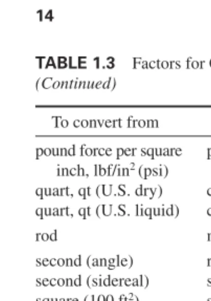
TABLE 1.3 Factors for Conversion to SI Units of Measurement (Continued)
To convert from To Multiply by
pound force per square pascal, Pa 6.894757 E03 inch, lbf/in2 (psi)
quart, qt (U.S. dry) cubic meter, m3 1.101221 E03
quart, qt (U.S. liquid) cubic meter, m3 9.463529 E04
rod meter, m 5.029210 E00
second (angle) radian, rad 4.848137 E06 second (sidereal) second, s 9.972696 E01 square (100 ft2) square meter, m2 9.290304† E00
ton (assay) kilogram, kg 2.916667 E02 ton (long, 2240 lb) kilogram, kg 1.016047 E03 ton (metric) kilogram, kg 1.000000† E03
ton (refrigeration) watt, W 3.516800 E03 ton (register) cubic meter, m3 2.831685 E00
ton (short, 2000 lb) kilogram, kg 9.071847 E02 ton (long per cubic kilogram per cubic 1.328939 E03
yard, ton)/yd3 meter, kg/m3
ton (short per cubic kilogram per cubic 1.186553 E03 yard, ton)/yd3 meter, kg/m3
ton force (2000 lbf) newton, N 8.896444 E03 tonne, t kilogram, kg 1.000000† E03
watt hour, Wh joule, J 3.600000† E03
yard, yd meter, m 9.144000† E01
square yard, yd2 square meter, m2 8.361274 E01
cubic yard, yd3 cubic meter, m3 7.645549 E01
year (365 days) second, s 3.153600† E07
year (sidereal) second, s 3.155815 E07
†Exact value.
From E380, “Standard for Metric Practice,” American Society for Testing and Materials.
CHAPTER 2
BEAM
FORMULAS
In analyzing beams of various types, the geometric proper-ties of a variety of cross-sectional areas are used. Figure 2.1 gives equations for computing area A, moment of inertia I,
section modulus or the ratio SI/c,where cdistance from the neutral axis to the outermost fiber of the beam or other member. Units used are inches and millimeters and their powers. The formulas in Fig. 2.1 are valid for both USCS and SI units.
Handy formulas for some dozen different types of beams are given in Fig. 2.2. In Fig. 2.2, both USCS and SI units can be used in any of the formulas that are applicable to both steel and wooden beams. Note that Wload, lb (kN); Llength, ft (m); Rreaction, lb (kN); Vshear, lb (kN); Mbending moment, lbft (Nm); D deflec-tion, ft (m); aspacing, ft (m); bspacing, ft (m); E modulus of elasticity, lb/in2 (kPa); Imoment of inertia,
in4(dm4); less than; greater than.
Figure 2.3 gives the elastic-curve equations for a variety of prismatic beams. In these equations the load is given as
P, lb (kN). Spacing is given as k, ft (m) and c, ft (m).
CONTINUOUS BEAMS
Continuous beams and frames are statically indeterminate. Bending moments in these beams are functions of the geometry, moments of inertia, loads, spans, and modulus of elasticity of individual members. Figure 2.4 shows how any span of a continuous beam can be treated as a single beam, with the moment diagram decomposed into basic com-ponents. Formulas for analysis are given in the diagram. Reactions of a continuous beam can be found by using the formulas in Fig. 2.5. Fixed-end moment formulas for beams of constant moment of inertia (prismatic beams) for
17
FIGURE 2.1
Geometric properties of sections.
18
19
FIGURE 2.1
(
Continued
)
Geometric properties of sections.
20
21
FIGURE 2.1
(
Continued
)
Geometric properties of sections.
22
23
FIGURE 2.1
(
Continued
)
Geometric properties of sections.
24
25
FIGURE 2.1
(
Continued
)
Geometric properties of sections.
26
FIGURE 2.1
(
Continued
)
Geometric properties of sections.
several common types of loading are given in Fig. 2.6. Curves (Fig. 2.7) can be used to speed computation of fixed-end moments in prismatic beams. Before the curves in Fig. 2.7 can be used, the characteristics of the loading must be computed by using the formulas in Fig. 2.8. These include , the location of the center of gravity of the load-ing with respect to one of the loads; G2 Pn/W, where bnL is the distance from each load Pn to the center of
gravity of the loading (taken positive to the right); and S3 Pn/W. These values are given in Fig. 2.8 for some
com-mon types of loading.
Formulas for moments due to deflection of a fixed-end beam are given in Fig. 2.9. To use the modified moment distribution method for a fixed-end beam such as that in Fig. 2.9, we must first know the fixed-end moments for a beam with supports at different levels. In Fig. 2.9, the right end of a beam with span Lis at a height dabove the left
end. To find the fixed-end moments, we first deflect the beam with both ends hinged; and then fix the right end, leaving the left end hinged, as in Fig. 2.9b. By noting that a
line connecting the two supports makes an angle approxi-mately equal to d/L(its tangent) with the original position
of the beam, we apply a moment at the hinged end to pro-duce an end rotation there equal to d/L.By the definition of
stiffness, this moment equals that shown at the left end of Fig. 2.9b. The carryover to the right end is shown as the top
formula on the right-hand side of Fig. 2.9b. By using the
law of reciprocal deflections, we obtain the end moments of the deflected beam in Fig. 2.9 as
28
29
30
31
FIGURE 2.2
(
Continued
)
Beam formulas.
32
33
FIGURE 2.2
(
Continued
)
Beam formulas.
34
35
FIGURE 2.2
(
Continued
)
Beam formulas.
36
37
FIGURE 2.2
(
Continued
)
Beam formulas.
38
39
FIGURE 2.2
(
Continued
)
Beam formulas.
40
FIGURE 2.3 Elastic-curve equations for prismatic beams. (a) Shears, moments, deflections for full
uni-form load on a simply supported prismatic beam. (b) Shears and moments for uniform load over part of
a simply supported prismatic beam. (c) Shears, moments, deflections for a concentrated load at any point
41
42
43
44
45
46
47
48
FIGURE 2.3 (Continued) Elastic-curve equations for prismatic beams. (q) Beam fixed at both ends—
49
50 CHAPTER TWO
BEAM FORMULAS 51
FIGURE 2.6 Fixed-end moments for a prismatic beam. (a) For a
concentrated load. (b) For a uniform load. (c) For two equal
con-centrated loads. (d) For three equal concentrated loads.
In a similar manner the fixed-end moment for a beam with one end hinged and the supports at different levels can be found from
(2.3)
where Kis the actual stiffness for the end of the beam that
is fixed; for beams of variable moment of inertia Kequals
the fixed-end stiffness times (1CLFCRF).
MFKd
FIGURE 2.7 Chart for fixed-end moments due to any type of
loading.
BEAM FORMULAS 53
FIGURE 2.8 (Continued) Characteristics of loadings.
ULTIMATE STRENGTH OF
CONTINUOUS BEAMS
Methods for computing the ultimate strength of continuous beams and frames may be based on two theorems that fix upper and lower limits for load-carrying capacity:
1. Upper-bound theorem. A load computed on the basis of
54 CHAPTER TWO
FIGURE 2.9 Moments due to deflection of a fixed-end beam.
2. Lower-bound theorem. The load corresponding to an
equilibrium condition with arbitrarily assumed values for the redundants is smaller than, or at best equal to, the ultimate loading—provided that everywhere moments do not exceed MP. The equilibrium method, based on
BEAM FORMULAS 55
For the continuous beam in Fig. 2.10, the ratio of the plastic moment for the end spans is ktimes that for the
cen-ter span (k 1).
Figure 2.10bshows the moment diagram for the beam
made determinate by ignoring the moments at Band Cand
the moment diagram for end moments MBand MCapplied
to the determinate beam. Then, by using Fig. 2.10c,
equilib-rium is maintained when
(2.4)
The mechanism method can be used to analyze rigid frames of constant section with fixed bases, as in Fig. 2.11. Using this method with the vertical load at midspan equal to 1.5 times the lateral load, the ultimate load for the frame is 4.8MP/Llaterally and 7.2MP/Lvertically at midspan.
Maximum moment occurs in the interior spans ABand CDwhen
(2.5) or if
(2.6)
A plastic hinge forms at this point when the moment equals
kMP. For equilibrium,
56 CHAPTER TWO
57
leading to
(2.7)
When the value of MPpreviously computed is substituted,
from which k0.523. The ultimate load is
(2.8)
In any continuous beam, the bending moment at any section is equal to the bending moment at any other section, plus the shear at that section times its arm, plus the product of all the intervening external forces times their respective arms. Thus, in Fig. 2.12,
Table 2.1 gives the value of the moment at the various supports of a uniformly loaded continuous beam over equal
BEAM FORMULAS 59
FIGURE 2.12 Continuous beam.
FIGURE 2.13 Relation between moment and shear diagrams for
a uniformly loaded continuous beam of four equal spans.
spans, and it also gives the values of the shears on each side of the supports. Note that the shear is of the opposite sign on either side of the supports and that the sum of the two shears is equal to the reaction.
60
TABLE 2.1 Uniformly Loaded Continuous Beams over Equal Spans
(Uniform load per unit lengthw; length of each spanl)
Distance to
point of Distance to
Shear on each side max moment, point of
Notation of support. Lleft, measured to inflection, Number of Rright. Reaction at Moment Max right from measured to
of support any support is LR over each moment in from right from
supports of span L R support each span support support
2 1 or 2 0 0 0.125 0.500 None
3 1 0 0 0.0703 0.375 0.750
2 0.0703 0.625 0.250
4 1 0 0 0.080 0.400 0.800
2 0.025 0.500 0.276, 0.724
1 0 0 0.0772 0.393 0.786
5 2 0.0364 0.536 0.266, 0.806
3 0.0364 0.464 0.194, 0.734
61
6 2 0.0332 0.526 0.268, 0.783
3 0.0461 0.500 0.196, 0.804
1 0 0 0.0777 0.394 0.788
2 0.0340 0.533 0.268, 0.790
7 3 0.0433 0.490 0.196, 0.785
4 0.0433 0.510 0.215, 0.804
1 0 0 0.0778 0.394 0.789
8 2 0.0338 0.528 0.268, 0.788
3 0.0440 0.493 0.196, 0.790
4 0.0405 0.500 0.215, 0.785
Values apply to wl wl wl2 wl2 l l
The numerical values given are coefficients of the expressions at the foot of each column.
62 CHAPTER TWO
inflection. Figure 2.14 shows the values of the functions for a uniformly loaded continuous beam resting on three equal spans with four supports.
Maxwell’s Theorem
When a number of loads rest upon a beam, the deflection at any point is equal to the sum of the deflections at this point due to each of the loads taken separately. Maxwell’s theo-rem states that if unit loads rest upon a beam at two points,
Aand B, the deflection at Adue to the unit load at Bequals
the deflection at Bdue to the unit load at A.
Castigliano’s Theorem
This theorem states that the deflection of the point of application of an external force acting on a beam is equal
FIGURE 2.14 Values of the functions for a uniformly loaded
BEAM FORMULAS 63
to the partial derivative of the work of deformation with respect to this force. Thus, if Pis the force,fis the
deflec-tion, and Uis the work of deformation, which equals the
resilience:
According to the principle of least work, the
deforma-tion of any structure takes place in such a manner that the work of deformation is a minimum.
BEAMS OF UNIFORM STRENGTH
Beams of uniform strength so vary in section that the unit stress Sremains constant, and I/cvaries as M. For
rectangu-lar beams of breadth band depth d,I/cI/cbd2/6 and MSbd2/6. For a cantilever beam of rectangular cross
sec-tion, under a load P,PxSbd2/6. If bis constant,d2varies
with x, and the profile of the shape of the beam is a parabola,
as in Fig. 2.15. If dis constant,bvaries as x,and the beam
is triangular in plan (Fig. 2.16).
Shear at the end of a beam necessitates modification of the forms determined earlier. The area required to resist shear is P/Svin a cantilever and R/Svin a simple beam.
Dot-ted extensions in Figs. 2.15 and 2.16 show the changes nec-essary to enable these cantilevers to resist shear. The waste in material and extra cost in fabricating, however, make many of the forms impractical, except for cast iron. Figure 2.17 shows some of the simple sections of uniform strength. In none of these, however, is shear taken into account.
64 CHAPTER TWO
SAFE LOADS FOR BEAMS
OF VARIOUS TYPES
Table 2.2 gives 32 formulas for computing the approximate safe loads on steel beams of various cross sections for an allowable stress of 16,000 lb/in2 (110.3 MPa). Use these formulas for quick estimation of the safe load for any steel beam you are using in a design.
BEAM FORMULAS 65
FIGURE 2.16 Triangular beam of uniform strength.
TABLE 2.2 Approximate Safe Loads in Pounds (kgf) on Steel Beams*
(Beams supported at both ends; allowable fiber stress for steel, 16,000 lb/in2(1.127 kgf/cm2) (basis of table)
for iron, reduce values given in table by one-eighth)
Greatest safe load, lb‡ Deflection, in‡
Shape of section Load in middle Load distributed Load in middle Load distributed
Solid rectangle
Hollow rectangle
Solid cylinder
Hollow cylinder wL3
67
Even-legged angle or tee
Channel or Z bar
68
TABLE 2.3 Coefficients for Correcting Values in Table 2.2 for Various Methods of Support and of Loading†
Max relative deflection under Max relative max relative safe
Conditions of loading safe load load
Beam supported at ends
Load uniformly distributed over span 1.0 1.0
Load concentrated at center of span 0.80
Two equal loads symmetrically concentrated l/4c
Load increasing uniformly to one end 0.974 0.976
Load increasing uniformly to center 0.96
Load decreasing uniformly to center 3兾 1.08
69
Beam fixed at one end, cantilever
Load uniformly distributed over span 2.40
Load concentrated at end 3.20
Load increasing uniformly to fixed end 1.92
Beam continuous over two supports equidistant from ends Load uniformly distributed over span
1. If distance a 0.2071l l2/4a2
2. If distance a0.2071l l/(l –4a)
3. If distance a0.2071l 5.83
Two equal loads concentrated at ends l/4a
†llength of beam; cdistance from support to nearest concentrated load; adistance from support to end
of beam.
70
71
FIGURE 2.17
Beams of uniform strength (in bending).
72
73
FIGURE 2.17
(
Continued
)
Beams of uniform strength (in bending).
74
75
FIGURE 2.17
(
Continued
)
Beams of uniform strength (in bending).
76
77
FIGURE 2.17
(
Continued
)
Beams of uniform strength (in bending).
78
FIGURE 2.17
(
Continued
)
Beams of uniform strength (in bending).
BEAM FORMULAS 79
ROLLING AND MOVING LOADS
Rolling and moving loads are loads that may change their position on a beam or beams. Figure 2.18 shows a beam with two equal concentrated moving loads, such as two wheels on a crane girder, or the wheels of a truck on a bridge. Because the maximum moment occurs where the shear is zero, the shear diagram shows that the maximum moment occurs under a wheel. Thus, with xa/2:
M2max when x a
M1max when x a
Figure 2.19 shows the condition when two equal loads are equally distant on opposite sides of the center of the beam. The moment is then equal under the two loads.
80
FIGURE 2.18 Two equal concentrated moving loads.
BEAM FORMULAS 81
If two moving loads are of unequal weight, the condi-tion for maximum moment is the maximum moment occur-ring under the heavier wheel when the center of the beam bisects the distance between the resultant of the loads and the heavier wheel. Figure 2.20 shows this position and the shear and moment diagrams.
When several wheel loads constituting a system are on a beam or beams, the several wheels must be examined in turn to determine which causes the greatest moment. The position for the greatest moment that can occur under a given
wheel is, as stated earlier, when the center of the span bisects the distance between the wheel in question and the resultant of all loads then on the span. The position for max-imum shear at the support is when one wheel is passing off the span.
CURVED BEAMS
The application of the flexure formula for a straight beam to the case of a curved beam results in error. When all “fibers” of a member have the same center of curvature, the concentric or common type of curved beam exists
(Fig. 2.21). Such a beam is defined by the Winkler–Bach theory. The stress at a point y units from the centroidal
axis is
Mis the bending moment, positive when it increases
curva-ture; yis positive when measured toward the convex side; A
is the cross-sectional area; Ris the radius of the centroidal
axis; Z is a cross-section propertydefined by
Analyticalexpressions for Zof certain sections are given
in Table 2.4. Zcan also be found by graphicalintegration
methods (see any advanced strength book). The neutral surfaceshifts toward the center of curvature, or inside fiber,
83
TABLE 2.4 Analytical Expressions for Z
Section Expression
A2 [(tb)C1bC2]
Z 1 R A
冤
b ln冢
RC2
RC2
冣
(tb) ln
冢
RC1 RC1冣
冥
and AtC1(bt) C3bC2
Z 1 R
A
冤
t ln (RC1)(bt) ln (RC0)b ln (RC2)冥
Z 12冢
Rr
冣
冤
R r√
冢
R r
冣
2
1
冥
Z 1 Rtheory, though practically satisfactory, disregards radial stresses as well as lateral deformations and assumes pure bending. The maximum stressoccurring on the inside fiber
is SMhi/AeRi, whereas that on the outside fiber is S
Mh0/AeR0.
The deflection in curved beams can be computed by
means of the moment-area theory. The resultant deflection is then equal to
in the direction defined by Deflections can also be found conveniently by use of Castigliano’s theorem.
It states that in an elastic system the displacement in the direction of a force (or couple) and due to that force (or cou-ple) is the partial derivative of the strain energy with respect to the force (or couple).
A quadrant of radius Ris fixed at one end as shown in
Fig. 2.22. The force Fis applied in the radial direction at
free-end B. Then, the deflection of Bis
tan y/ x.
0
√
2x 2yFIGURE 2.21 Curved beam.
By moment area,
FIGURE 2.22 Quadrant with fixed end.
Eccentrically Curved Beams
These beams (Fig. 2.23) are bounded by arcs having differ-ent cdiffer-enters of curvature. In addition, it is possible for either radius to be the larger one. The one in which the section depth shortens as the central section is approached may be called the arch beam. When the central section is the
largest, the beam is of the crescent type.
Crescent Idenotes the beam of larger outside radius and crescent IIof larger inside radius. The stress at the central section of such beams may be found from SKMC/I.
In the case of rectangular cross section, the equation becomes S6KM/bh2, where Mis the bending moment,b
is the width of the beam section, and hits height. The stress factors,Kfor the inner boundary, established from
photo-elastic data, are given in Table 2.5. The outside radius
86 CHAPTER TWO
BEAM FORMULAS 87
TABLE 2.5 Stress Factors for Inner Boundary at Central Section
(see Fig. 2.23)
1. For the arch-type beams
(a)
(b)
(c) In the case of larger section ratios use the equivalent beam solution
2. For the crescent I-type beams
(a)
(b)
(c)
3. For the crescent II-type beams
(a)
crescent beams is such that the stress can be larger in off-center sections. The stress at the central section determined
88 CHAPTER TWO
given in Table 2.6. As in the concentric beam, the neutral surface shifts slightly toward the inner boundary. (See
Vidosic, “Curved Beams with Eccentric Boundaries,”
Transactions of the ASME,79, pp. 1317–1321.)
ELASTIC LATERAL BUCKLING OF BEAMS
When lateral buckling of a beam occurs, the beam under-goes a combination of twist and out-of-plane bending (Fig. 2.24). For a simply supported beam of rectangular cross section subjected to uniform bending, buckling occurs at the critical bending moment, given by
where Lunbraced length of the member
Emodulus of elasticity
Iymoment of inertial about minor axis
Gshear modulus of elasticity
Jtorsional constant
The critical moment is proportional to both the lateral bending stiffness EIy/L and the torsional stiffness of the
member GJ/L.
For the case of an open section, such as a wide-flange or I-beam section, warping rigidity can provide additional tor-sional stiffness. Buckling of a simply supported beam of open cross section subjected to uniform bending occurs at the critical bending moment, given by
TABLE 2.6 Crescent-Beam Position Stress Factors
(see Fig. 2.23)†
Angle , k
degree Inner Outer
10 10.055 H/h 10.03 H/h
†Note: All formulas are valid for 0 H/h0.325. Formulas for the inner
boundary, except for 40 degrees, may be used to H/h0.36. Hdistance between centers.
where Cw is the warping constant, a function of
cross-sectional shape and dimensions (Fig. 2.25).
In the preceding equations, the distribution of bending moment is assumed to be uniform. For the case of a nonuni-form bending-moment gradient, buckling often occurs at
90 CHAPTER TWO
FIGURE 2.24 (a) Simple beam subjected to equal end moments. (b) Elastic lateral buckling of the beam.
a larger critical moment. Approximation of this critical bending moment,Mcrmay be obtained by multiplying Mcr given by the previous equations by an amplification factor
where Cb
12.5Mmax
2.5Mmax3MA4MB3MC
BEAM FORMULAS 91
and Mmaxabsolute value of maximum moment in the unbraced beam segment
MAabsolute value of moment at quarter point of
the unbraced beam segment
MBabsolute value of moment at centerline of the
unbraced beam segment
MCabsolute value of moment at three-quarter
point of the unbraced beam segment FIGURE 2.25 Torsion-bending constants for torsional buckling.
Across-sectional area; Ixmoment of inertia about x–xaxis;
Iymoment of inertia about y–yaxis. (After McGraw-Hill, New
Cbequals 1.0 for unbraced cantilevers and for members
where the moment within a significant portion of the unbraced segment is greater than, or equal to, the larger of the segment end moments.
COMBINED AXIAL AND BENDING LOADS
For short beams, subjected to both transverse and axial loads, the stresses are given by the principle of superposition if the deflection due to bending may be neglected without serious error. That is, the total stress is given with sufficient accuracy at any section by the sum of the axial stress and the bending stresses. The maximum stress, lb/in2 (MPa),
equals
where Paxial load, lb (N)
Across-sectional area, in2(mm2)
Mmaximum bending moment, in lb (Nm)
cdistance from neutral axis to outermost fiber at the section where maximum moment occurs, in (mm)
Imoment of inertia about neutral axis at that section, in4(mm4)
When the deflection due to bending is large and the axial load produces bending stresses that cannot be neglect-ed, the maximum stress is given by
f P
A
Mc I
BEAM FORMULAS 93
where dis the deflection of the beam. For axial
compres-sion, the moment Pdshould be given the same sign as M;
and for tension, the opposite sign, but the minimum value of MPdis zero. The deflection dfor axial compression
and bending can be closely approximated by
where dodeflection for the transverse loading alone, in
(mm); and Pccritical buckling load 2EI/ L2, lb (N).
UNSYMMETRICAL BENDING
When a beam is subjected to loads that do not lie in a plane containing a principal axis of each cross section, unsym-metrical bending occurs. Assuming that the bending axis of the beam lies in the plane of the loads, to preclude torsion, and that the loads are perpendicular to the bending axis, to preclude axial components, the stress, lb/in2(MPa), at any
point in a cross section is
where Mxbending moment about principal axis XX,
in lb (Nm)
Mybending moment about principal axis YY,
94 CHAPTER TWO
xdistance from point where stress is to be computed to YYaxis, in (mm)
ydistance from point to XXaxis, in (mm)
Ixmoment of inertia of cross section about XX,
in (mm4)
Iymoment of inertia about YY, in (mm4)
If the plane of the loads makes an angle with a principal plane, the neutral surface forms an angle with the other principal plane such that
ECCENTRIC LOADING
If an eccentric longitudinal load is applied to a bar in the
plane of symmetry, it produces a bending moment Pe,
where eis the distance, in (mm), of the load P from the
centroidal axis. The total unit stress is the sum of this moment and the stress due to Papplied as an axial load:
where Across-sectional area, in2(mm2)