A HYBRID TRANSFER FUNCTION AND ARTIFICIAL NEURAL NETWORK MODEL FOR TIME SERIES FORECASTING - ITS Repository

(1)

Thesis-SS14 2501

A HYBRID TRANSFER FUNCTION AND ARTIFICIAL

NEURAL NETWORK MODEL FOR TIME SERIES

FORECASTING

FAHMI (1314201210)

Supervisors

1. Dr. BRODJOL SUTIJO S.U., M.Si. 2. Dr. SUHARTONO

Master Program

Department of Statistics

Faculty of Mathematics and Natural Sciences Institut Teknologi Sepuluh Nopember

(2)

(3)

List of Tables

(6)

(7)

List of Figures

2.1 Input to, and Output from, a Dynamic System by Box and Jenkins . . 15

2.2 Prewhitening Step-by-Step . . . 16

2.3 A Basic Multiple Input Artificial Neuron Model . . . 25

2.4 Radial Basis Function Neural Networks Architecture . . . 27

2.5 Hybrid Model . . . 32

3.1 Representative Offices of Indonesian Central Bank (BI) in Aceh Province 37 3.2 Inflow (in Billion IDR) - Lhokseumawe and Banda Aceh . . . 38

3.3 Outflow (in Billion IDR) - Lhokseumawe and Banda Aceh . . . 38

3.4 Consumer Price Index (CPI) - Lhokseumawe and Banda Aceh . . . 39

4.1 Time Series plots of Differenced CPI, ACF, and PACF of Lhokseumawe 45 4.2 Actual vs Transfer Function-Noise prediction of Outflow Lhokseumawe 47 4.3 Actual vs Hybrid prediction of Outflow Lhokseumawe . . . 47

4.4 Actual vs Transfer Function-Noise prediction of Inflow Lhokseumawe-Model 1 . . . 50

4.5 Actual vs Hybrid prediction of Inflow Lhokseumawe-Model 1 . . . 50

4.6 Time Series plots of Differenced CPI, ACF, and PACF of Banda Aceh . 51 4.7 Actual vs Transfer Function-Noise prediction of Outflow Banda Aceh . 53 4.8 Actual vs Hybrid prediction of Outflow Banda Aceh . . . 53

4.9 Actual vs Transfer Function-Noise prediction of Outflow Banda Aceh . 55 4.10 Actual vs Hybrid prediction of Inflow Banda Aceh . . . 56

(8)

(9)

List of Abbreviations

ARIMA Autoregressive Integrated Moving Average ACF Autocorrelation Function

CPI Consumer Price Index CCF Cross Correlation Function

HP Hybrid Prediction

MAD Mean Average Deviation

PACF Partial Autocorrelation Function RBF Radial Basis Function

(10)

(11)

A HYBRID TRANSFER FUNCTION AND ARTIFICIAL NEURAL NETWORK MODEL FOR TIME SERIES FORECASTING

By : FAHMI

Student Identity Number : 1314201210

Supervisors : 1. Dr. BRODJOL SUTIJO S.U., M.Si.

Supervisor : 2. Dr. SUHARTONO

ABSTRACT

In finance and banking, the ability to accurately predict the future cash require-ment is fundarequire-mental to many decision activities. In this research, we study time series forecasting of cash inflow and outflow requirements as the output series of Indonesian Central Bank (BI) at the representative offices in Aceh Province, Indonesia. We use a Consumer Price Index (CPI) as the leading indicator of the input series to predict the output series. A CPI measures change in the price level of a market basket of consumer goods and services purchased by households. CPI has been used in time series modeling as a good predictor for response. In this study, we propose a hybrid approach to forecast the cash inflow and outflow by combining linear and non linear models. This methodology combines both Transfer Function and Radial Basis Func-tion (RBF) Neural Network models. The idea behind this model is the time series are rarely pure linear or nonlinear parts in practical situations. The RBF neural network is used to develop a prediction model of the residual from Transfer Function model. The RBF Neural Networks model is trained by Gaussian activation function in hidden layer. The main concept of the proposed hybrid model approach is to let the Transfer Function forms the linear component and let the neural network forms the nonlinear component and then combine the results from both linear and nonlinear models. This combination model provides a better forecast accuracy than the individual linear or non linear model. This combination model is expected to provide a better forecast accuracy thanxxx

Keywords: Inflow, Outflow, Consumer Price Index, Transfer Function, Artificial

(12)

(13)

CHAPTER 1 INTRODUCTION

1.1 Background

(14)

and other fiscal policies (Bank Indonesia, 2014). Fisher, Liu and Zhou (2002) stated that one of the important things for making monetary decisions is the forecasting of inflation. So far, BPS of Indonesia uses CPI as an indicator to measure the level of inflation in Indonesia. Therefore, the forecasting of inflation can be approached by modeling the forecasting of CPI.

The appropriate time series forecasting methodology plays an important role to meet the accurate future values. Time series modeling approach is the major tech-niques widely used in practice. Time series methods, on the other hand, use past or lagged values of the same criterion variable and model the relationship between these past observations and the future value. Autoregressive Integrated Moving Average (ARIMA) is one of the most important and popular linear models in time series fore-casting a few decades ago. This model was popularized by Box and Jenkins (1976). Due to its statistical properties, ARIMA is also called the Box-Jenkins model particu-larly in the model building process. Although ARIMA models are the effective method to study time series with one time series in systems and widely used in time series forecasting, their major limitation is unable to express well the relationships in multi-variate time series among variables in system (Zhang, 2003). So it is necessary to model a time series with multivariable models (Fan, Shan, Cao, and Li, 2009). Many different mathematical presentations of Transfer Function models can be found in the literature (Pektas and Cigizoglu, 2013). Transfer Function models have found extensive practical application. In Box and Jenkins methodology, ARIMA and Transfer Function model building follow the standard procedures.

(15)

and Zhang, (2010) and many other real world applications like Analysis of Groundwa-ter by Ding, Liu, and Zhao, (2010), Wind Energy Forecasting by Campbell, Ahmed, Fathulla, and Jaffar, (2010), RBF by Mohammadi, Ghomi, Zeinali (2014), Traffic vol-ume forecasting by Zhu, Cao, and Zhu (2014). Furthermore, Du, Leung, and Kwong (2014) shown that the distribution of the ANN in multi objective evolutionary algo-rithm produced the best forecast results.

In this study, we propose a hybrid approach to forecast the cash inflow and out-flow using both Transfer Function and Radial Basis Function (RBF) Neural Network models. Numerous efforts have been introduced for developing and improving time series forecasting methods. In practical situations, time series are rarely pure linear or nonlinear components. However, the linear nature of the transfer function model is inappropriate to capture nonlinear structure of time series data, where the residuals of linear model contain information about the nonlinearity. Since it is difficult to com-prehensively know the data characteristics whether a time series is generated from a linear or nonlinear process in a real world, hybrid methodology is proposed in practice (Zhang, 2003).

Makridakis and Hibon (2000) concluded in their paper of M3-competitions: re-sults, conclusions and implications point 3 that combination is more accurate than the individual methods being combined for practically all forecasting horizons. Six years later, De Gooijer and Hyndman (2006) concluded in their paper of25th years of time series forecasting that combination method for linear and nonlinear models is an important practical issue that will no doubt receive further research attention in the future. Therefore, combining different models become so popular in practice due to the ability of capturing different patterns in the data and nice forecasting performance. Combining model in time series forecasting can significantly improve the forecasting performance over each individual model used separately (Zhang, 2003; Zhang, 2004; Robles et al., 2008; Shukur and Lee, 2015; Khandelwal, Adhikari, and Verma 2015)

(16)

accurately model the complex autocorrelation structures in the data. Based on Zhang’s hybrid model (Zhang, 2003 and 2004), the methodology of the hybrid system consists of two steps. In the first step, an Transfer Function is used to analyze the linear part of the problem. In the second step, an RBF Neural Network model is developed to model the residuals from the Transfer Function. Since the Transfer Function model cannot capture the non linear structure of the data, the residuals of linear model will contain information about the non linearity. The results from RBF Neural Network can be used as predictions of the error terms for the Transfer Function model.

This research paper contains five chapters, which are organized as follows: Chap-ter 2 provides a related liChap-terature review on the basic concepts of time series analysis like stationarity, differencing, the theory of Transfer Function, Neural Network, Hybrid model, Forecasting, etc. are also stated in this chapter. In chapter 3 we present the location of research area, data, variables, and research methods. Section 4 displays and discusses the empirical results and the conclusions are provided in the last section.

1.2 Problem Statement

Based on the background described above, we want to figure out the following problem formulations:

1. How to obtain the appropriate Transfer Function-noise model to forecast the cash inflow and outflow of Indonesian Central Bank (BI) at representative offices in Aceh Province by using input variable Consumer Price Index (CPI).

2. How to obtain the appropriate RBF Neural Network for forecasting residual of Transfer Function

(17)

1.3 Purpose of Study

The objective of this research is to forecast cash inflow and outflow of Indonesian Central Bank using the hybrid Transfer Function and Radial Basis Function Neural Network time series model. This approach is valuable because time series are rarely pure linear or nonlinear components in practical situations.

1.4 Limitation of Study

Although this research was carefully prepared, we still aware of its limitations and shortcomings:

1. Numerous methods for selecting forecast combination have been proposed. For instance, the simple linear combination, non linear combination, and the mixture of linear and non linear combination. In this research we only restrict to the combination of linear (Transfer Function) and non linear (Radial Basis Function Neural Network) methods.

(18)

(19)

CHAPTER 2 LITERATURE REVIEW

xxxThe primary objective of time series analysis is to develop mathematical models that provide plausible descriptions for sample data. In this research, a time series

y1, . . . , yT are assumed to be generated by a collection of random variables with prob-ability structure (stochastic processes)_{yt_}_t∈_T, where T is an index set containing the

subset 1, . . . , T, the subscripts t are usually thought of as representing time or time periods (L¨utkepohl and Kr¨atzig, 2004).

The mathematical model which is used in this research is the Hybrid system of Transfer Function and Radial Basis Function Neural Network models. For the pur-pose of forecasting, the basic concepts of Autoregressive Integrated Moving Average (ARIMA) model is required due to its statistical properties as well as the well known Box and Jenkins methodology in the model building process. The other necessary con-cepts considered in this research are White Noise, Autocorrelation Function (ACF), Partial Autocorrelation Function (PACF), and Cross Correlation Function (CCF).

2.1 Autoregressive Integrated Moving Average (ARIMA)

Box and Jenkins (1976) and Wei (2006) define the autoregressive or self-regressive process of order p (AR(p)) as

˙

yt =ϕ1yt˙−1+ϕ2yt˙−2+· · ·+ϕpyt˙−p+εt (2.1)

or by using the lag operator

ϕp(L) ˙y=εt, (2.2)

where ϕp(L) = (1₋ϕ1L₋ϕ2L2_{− · · · −}_ϕpLp_{), and ˙}_yt ₌ _yt₋_µ_{. The analogy to the}

moving average process of orderq, denoted as MA(q) can be written

˙

(20)

or by using the lag operator

˙

yt=θ(L)εt, (2.4)

whereθ(L) = 1₋θ1L₋θ2L2 _{− · · · −}_θqLq_.

A mixed ARMA process yt with AR order p and MA order q (ARMA(p, q)) has the representation

˙

yt=ϕ1yt˙−1+ϕ2yt˙−2+· · ·+ϕpyt˙−p+εt−θ1εt−1−θ2εt−2− · · · −θqεt−q (2.5)

or by using the lag operator can be written

ϕp(L) ˙y =θq(L)εt, (2.6)

A stochastic process yt is called an ARIMA(p,d,q) process (yt _∼ ARIMA(p,d,q)) if it is I(d) and the d times difference process has an ARMA(p,q) representation, that is ∆d_yt _∼ _ARMA(_p,q_{) (L¨}_{utkepohl and Kr¨atzig, 2004). For practical purposes,} _d _is

usually equal to 1 or at most 2. It is important that the number of difference in ARIMA is written differently even though referring to the same model. Time seriesyt

is said to follow an integrated autoregressive moving average model if the dth differ-enceW t = ∆d_yt _{is a stationary ARMA process (Cryer and Chan, 2008). For example,}

ARIMA(1,1,0) of the original series can be written as ARMA(1,0,0) of the differenced series.

2.2 Stationarity and Differencing

2.2.1 Stationarity

The basis for any time series analysis is stationary time series. A stochastic process

yt is called stationary if it has time-invariant first and second moments (L¨utkepohl and Kr¨atzig, 2004). In other words, yt is stationary if

xxxE[yt] = µy for all t _∈ T and

xxxE[(yt₋µy)(yt−h−µy)] =γh for all t ∈ T and all integersh such thatt-h ∈T.

(21)

mean and variance. More specifically, there are two definitions of stationary stochastic processes that are sometimes used in the literature: strictly stationary and weakly stationary.

A processYtis said to bestrictly stationary if the joint distribution ofyt1, yt2, . . . , ytn

is the same as the joint distribution of yt1−k, yt2−k, . . . , ytn−k for all choices of time

points t1, t2, . . . tn and all choices of time lag k (Hamilton, 1994). A less restrictive requirement of stochastic process yt is considered by Kirchg¨assner and Wolters (2007) since the concept of strict stationary is difficult to apply in practice. This process is calledweakly stationary orcovariance stationary. A stochastic processyt having finite mean and variance is covariance stationary if for all t and t-s,

xxxE[yt] =E[yt−s] =µy xxxE[(yt₋µy)2_{] =}_E_[(_yt

−s−µy)2] =var(yt) =var(yt−s) = σy2 xxxE[(yt₋µy)(yt−s−µy)] = E[(yt−j −µy)(yt−j−s−µy)] xxxxxxxxxxxxxxxxxxxx.=Cov(yt, yt−s)

xxxxxxxxxxxxxxxxxxxx.=Cov(yt−j, yt−j−s) =γs,

where µy, σ2

y, and all γs are constants (Box and Jenkins, 1976; Hamilton, 1994; and

Enders, 2009).

For example, Hamilton (1994) shown that since the mean and autocovariances are not function of time, MA(1) process is weakly stationary regardless of the values ofθ. In the case when_|ϕ_|<1, AR(1) is also weakly stationary. In this research, we will use the term stationary as a weakly stationary where it is mean and covariance stationary.

2.2.2 Differencing

In practice, many time series are non-stationary and so we cannot apply stationary AR, MA or ARMA processes directly. One possible way of handling non-stationary series is to apply differencing so as to make them stationary (Chatfield, 2000). Dif-ferencing method governs the series to be lagged 1 step and subtracted from original series. For instance, (yt ₋yt−1) = (1− L)yt may themselves be differenced to give

second differences, and so on. The dth differences may be written as (1₋L)d_yt_.

(22)

expressed by ∆2_yt_{= ∆(∆}_yt_{) = (1}₋_L₎₍₁₋_L₎_yt_{= (1}₋₂_L₊_L2₎_yt_{= (}_yt₋₂_yt

−1+yt−2)

(Yafee and McGee, 1999).

2.3 White Noise

A stationary process, where all autocorrelations are zero is called white noise or a white noise process. Hamilton (1994) and Wei (2006) said a process εt is a white

noise process if it is a sequence of uncorrelated random variable from fixed distribution follows: E(εt) = 0, E(ε2t) = σ2, and for which the ε′s are uncorrelated across time, E(εtετ) = 0 for all t ₆=τ. Sinceεt and ετ are independent (uncorrelated) for allt ₆=τ, then εt ∼ N(0, σ2) which is also called Gaussian white noise process. The white noise

process εt may be regarded as a series of shocks which drive the system (Box and Jenkins, 1976)

2.4 Correlations

2.4.1 Autocorrelations

Autocovariances and autocorrelations are addiction measurements between vari-ables in a time series. Suppose thaty1, . . . , yT are square integrable random variables, then Falk (2006) and Montgomery, Jennings, and Kulahci (2008) defined the autoco-variance is the covariance between yt and its value at another time period yt−k

γk=Cov(yt, yt−k) =E[(yt−µy)(yt−k−µy)], k = 0,1,2, . . . , (2.7)

with the property that the covariance of observations with lag k does not depend on

t. The collection of the values of γk , k = 0, 1, 2, . . . is called the autocovariance

function. The autocovariance at lagk = 0 is just the variance of the time series; that is, γ0 = σy2. The autocorrelation between yt and its another time period yt−k can be

defined as

(23)

Thus, the autocorrelation coefficient at lagk is tion (ACF). In practice, the autocorrelation function from a time series of finite length

y1, y2, . . . , yT is estimated by the sample autocorrelation function (or sample ACF) rk. By usingy= _T1 PT_t=1 =µy as the sample mean, L¨utkepohl and Kr¨atzig (2004) compute the sample autocorrelations as follows

e

If the sample autocorrelations are mutually independent and identically distributed (i.i.d.) so that yt and yt−k are stochastically independent for k 6= 0, then the

nor-malized estimated autocorrelations are asymptotically standard normally distributed,

√

Tρk_e _−→d N(0,1), and thus ρk_e _≈ N(0,1/T). Hence, [₋1,96/p1/T; 1,96/p1/T] is an approximate 95% confidence interval around zero, where the variance of the sample autocorrelation coefficient isV ar(ρk_e )∼= 1/T and the standard error isSE(ρk_e )∼= 1/√T. For detail properties of autocovariance and autocorrelation see (Wei, 2006).

2.4.2 Partial Autocorrelations

L¨utkepohl and Kr¨atzig (2004) define the partial correlation between yt and yt−k is

the conditional autocorrelation given yt−1, yt−2, . . . , yt−k+1 as follows

φkk =Corr[yt, yt−k|yt−1, yt−2, . . . , yt−k+1] (2.12)

(24)

should be equal to zero. A more formal definition can be found below (Box and Jenkins, 1976; Wei, 2006; Kirchg¨assner and Wolters, 2007; and Montgomery et al., 2008). The Yule-Walker equations for the ACF of an AR(p) process for any fixed value of k is

(25)

φk =

with Cramer’s rule we have

φkk =

= 0 for k > p. Sample partial autocorrelation function,φbkk or some authors called the

sample estimate of φkkb is estimated as

(26)

Furthermore, in a sample of T observations from an AR(p) process, φkkb , for k > p is approximately normally distributed with

E[φkkb ]_≈0 and V ar(φkkb )_≈ 1 T

Hence the 95% critical limits to test whether anyφkkb is statistically significant different from zero are given by _±1,96/√T. For further detail and example could be seen in Wei (2006).

2.4.3 Cross-Correlation Function

For the bivariate time series, xt, yt, the cross-correlation function measures the strength and the direction of correlation between two random variables. In Transfer Function model, the shape of the cross-correlation between those input and output series reveals the pattern of (r, s, and b) parameters of the transfer function (Box and Jenkins, 1976). The two stationary stochastic processesxtandyt, fort= 0,_±1,_±2, . . . ,

have the following cross-covariance function

Cov(xt, yt) = γxy(k) =E[(xt₋µx)(yt+k₋µy)] (2.21)

fork = 0,_±1,_±2, . . . , where µx =E[xt] andµy =E[yt]. Hence Wei (2006) defined the

cross-correlation function (CCF) of the bivariate process as

ρxy(k) = γxy(k)

σxσy (2.22)

fork = 0,_±1,_±2, . . . , whereσx andσy are the standard deviations of xt and yt. For a given sample ofT observations of the bivariate process, the cross correlation function,

ρxy(k), is estimated by sample cross correlation

(27)

where n = T ₋d pairs of values (x1, y1),(x2, y2), . . . ,(xn, yn), Sx = p_bγxx(0) and

Sy =p_bγyy(0) available after differencing, and x and y are the sample mean of xt and

yt respectively.

2.5 Transfer Function Model

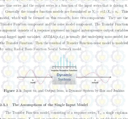
The relationship between the input series, Xt, and the output series, Yt, is a

func-tional process. The response may be delayed from one level to another and distributed over a period of time. Such relationships are called dynamic transfer functions. A dynamic system may exist where an input series seems related to an output series. Box and Jenkins (1976) illustrated a dynamic system of input and output series with impulse response function as shown in Figure 2.1. Both the input and output series are time series and the output series is a function of the input series that is driving it. Generally the transfer function models are formulated as Yt = v(L)Xt+nt. This model, which will be focused on this research, have two components. They are the Transfer Function component and the noise model component. The Transfer Function component consists of a response regressed on lagged autoregressive output variables and lagged input variables. ARIMA(p,d,q) is usually the underlying noise model for the Transfer Function. Then the residual of Transfer Function-noise model is modeled by using Radial Basis Function Neural Network model.

Figure 2.1: Input to, and Output from, a Dynamic System by Box and Jenkins

2.5.1 The Assumptions of the Single Input Model

(28)

are assumed stationary (Box and Jenkins, 1976; Wei, 2006). Therefore centered and differenced (if necessary) is required to attain a stationarity condition.

For the input modeling, an error term which may be autocorrelated, is usually assumed to be white noise (Bisgaard and Kulahci, 2011). The represent of the unob-servable noise process Nt, is assumed to be independent of the dynamic relationship between the output Yt and the input Xt (Montgomery et al., 2008). Moreover, Yafee and McGee (1999) presumed that this relationship is unidirectional with the direction of flow from the input to the output series. Therefore Xt in a Transfer Function must be input and the Transfer Function is assumed to be stable.

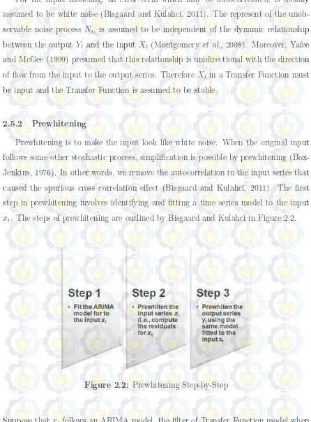
2.5.2 Prewhitening

Prewhitening is to make the input look like white noise. When the original input follows some other stochastic process, simplification is possible by prewhitening (Box-Jenkins, 1976). In other words, we remove the autocorrelation in the input series that caused the spurious cross correlation effect (Bisgaard and Kulahci, 2011). The first step in prewhitening involves identifying and fitting a time series model to the input

xt. The steps of prewhitening are outlined by Bisgaard and Kulahci in Figure 2.2.

Figure 2.2: Prewhitening Step-by-Step

(29)

(Montgomeryet al., 2008). For example, suppose that the sample of ACFand PACF indicate that the original input series Xt is non-stationary, but its differences xt = (1₋L)Xt are stationary. Then suppose the appropriate model might be a second order autoregressive AR(2) model

(1₋ϕ1L+ϕ2L2)xt=ϕ(L)xt=αt (2.25)

where xt = (1−L)Xt and the αt are the white noise process. After prewhitening the

input, the next step is to prewhiten the output Yt. The prewhitening filter for xt will be used to filter the differences output seriesyt= (1−L)Yt. This involves filtering the

output data through the same model with the same coefficient estimates that we fitted to the input data. The prewhitened output is

(1₋ϕ1L+ϕ2L2)yt =ϕ(L)yt=βt (2.26)

The process of transformingXttoαt and from Yt toβtvia the filter 1₋ϕ1L+ϕ2L2 ₌ ϕ(L) is known as whiteningor prewhitening (Cryer and Chan, 2008).

2.5.3 Identification of Transfer Function

The dynamic relationship between the outputYtand the inputXtusing the Transfer Function-Noise model for linear system is

Yt=v(L)Xt+Nt, (2.27)

where v(L) = P∞_j=0vjLj _{is Transfer Function filter and} _Nt _{is the noise series that}

is assumed to be independent of Xt and generated usually by an ARIMA process. However in our case Nt will be generated by non linear neural network process. If the series exhibits non-stationarity, an appropriate differencing is required to obtain stationaryxt, yt, and nt. Hence, the Transfer Function-Noise model becomes

(30)

and

v(L)_≈ ω(L)

δ(L)L

b _(2.29)

This imply that (2.27) can be written as

yt=v(L)xt+nt δ(L) in (2.30) determines the structure of the infinitely order, therefore the stability of

v(L) depends on the coefficients inδ(L). As an infinite series,v(L) converges as_|L_{| ≤}1 (Yafee and McGee, 1999; Mongomeryet al., 2008). v(L) is said to be stable under this condition, if all the roots of mr₋_δ1mr1 _{− · · · −}_δr _{are less than 1 in absolute value.}

When the transfer function is absolutely summable, it converges and is considered to be stable, then

∞ X

L=0

|v(L)_|<_∞ (2.31)

In the identification procedure, Wei (2006) derived the following simple steps to obtain the transfer function v(L):

1. Prewhiten the input series, ϕx(L)xt=θx(L)αt

i.e., αt= ϕx(L)

θx(L)

xt (2.32)

whereαt is a white noise series with mean zero and variance σ2α

2. Calculate the filtered output series. That is, transform the output seriesyt using the above prewhitening model to generate the series

βt =

ϕx(L)

θx(L)yt (2.33)

(31)

4. Identifyb, r, s, ω(L), δ(L) by matching the pattern of CCF. Onceb, r, sare chosen, preliminary estimates ωj_b and bδj can be found from their relationships with vk. Thus we have a preliminary estimates of the transfer functionv(L) as

b

v(L) = ωb(L)

b δ(L)L

b_. _(2.34)

The noise series of the transfer function can be estimated by

b

nt=yt₋_bv(L)xt

=yt₋ bω(L) b δ(L)L

b_xt. (2.35)

By examining the ACF and the PACF of_bnt, we have

ϕ(L)nt =θ(L)at (2.36)

By combining (2.34 ) and (2.36), the general form of transfer function-noise model is

yt= ω(L)

δ(L)xt−b+

θ(L)

ϕ(L)at. (2.37)

2.5.4 The Structure of the Transfer Function

The impulse response weightsvj consist of a ratio of a set ofs regression weights to a set of r decay rate weights, plus a lag level, b, associated with the input series, and may be expressed with parameters designated withr,s, andb subscripts, respectively. Box and Jenkins (1976) and Wei (2006) found the orders of r, s, and b and their relationships to the impulse response weightvj by equating the equations ofLb _{in both}

sides of the equation

δ(L)v(L) = ω(L)Lb (2.38) and we obtain the identity

(32)

Thus we have

xxxvj = 0 j < b,

xxxvj =δ1vj−1+δ2vj−2+· · ·+δrvj−r+ω0 j =b,

xxxvj =δ1vj−1+δ2vj−2+· · ·+δrvj−r−ωj−b j =b+ 1, b+ 2,· · · , b+s, xxxvj =δ1vj−1+δ2vj−2+· · ·+δrvj−r j > b+s.

The weightsvb+s, vb+s−1, . . . , vb+s−r+1 supplyr impulse response starting values for the

difference equation

δ(L)v

j

= 0,

j > b

+

s

(2.40)

In general, the impulse response vj consist of 1. b zero valuesv0, v1, . . . , vb−1

2. s₋r+ 1 weights vb, vb+1, . . . , vb+s−r that follows no fixed pattern

3. r starting impulse response weightsvb+s−r+1, vb+s−r+2, . . ., and vb+s

4. vj forj > b+s follows the pattern given in (2.39)

Yafee and McGee (1999) define the order b, r, sas follows: The delay timeb, some-times referred to as dead time, determines the pause before the input begins to have an effect on the response variable (L)b_Xt ₌_Xt

−b. The order of the regression s designates

the number of lags for unpatterned spikes in the transfer function. The number of unpatterned spikes is s+ 1. The order of decay r represents the patterned changes in the slope of the function. The order of this parameter signifies the number of lags of autocorrelation in the transfer function. The denominator of the transfer function ratio consists of decay weights,δr from time = 1 tor. If there is more than one decay

rate, the rate of contemplation may fluctuate.

2.5.5 Estimation of Transfer Function Model

(33)

at is N(0, σ2

a), it can be estimated by conditional least squares, unconditional least

squares, or maximum likelihood.

In this research, the parameter for single input Transfer Function-noise model is estimated by using conditional least square. For the linear model part, the δi and ωi

can be recursively estimated by using bδ(L)_bv(L) = ω_b(L) from (2.41) (Montgomery et

2.5.6 Diagnostic Checking of Transfer Function Model

To test the adequacy of a model, the estimated parameters should be significant. If the parameters are not significant, we drop them out from the model. In diagnostic checking step, Montgomery et al. (2008) checked the validity of two assumptions in the fitted model. These assumptions are: the noise at is white noise by examining the residual_bat through ACF and PACF pattern and the independence between_bat and

xt by observing the sample cross-correlation function between the residual αt from the prewhitened input and xt. To see whether these assumptions hold, Wei (2006) examined the residual _bat from the noise model as well as the residual αt:

1. Cross correlation check. For an adequate model, the sample CCF, ρα,_b _ba(k),

be-tween_ba and α should show no patterns and lie within their two standard errors 2(n₋k)−1/2_{. The Portmanteau test} _Q0 _{which approximately follows a}_χ2

distri-bution with (K+1)₋M degree of freedom can be used to check this assumptions.

(34)

where m=n₋t0 + 1, t0 =max_{p+r+ 1, b+p+s+ 1_}, M is the number of parametersδi and ωj, j = 0,1,2, . . . , K, and n is the number of residuals at.

2. Autocorrelation check. For an adequate model, both the sample ACF and PACF should not show any patterns. The Portmanteau test Q1 which approximately follows a χ2 _{distribution with}_K ₋_p₋_q _{degree of freedom can be used to check}

this assumptions.

2.5.7 The General Modeling Strategies for Transfer Function Model The procedure for modelling strategies of the transfer function model according to (Wei, 2006; Bisgaard and Kulahci, 2011; and Yafee and McGee, 1999) are as the following steps:

1. Plot the data. By graphing or plotting the input and output series, we will gain a preliminary overview of the general behavior of these variables. This step is also called preprocessing step. In this step, transformation of both input and output series into stationary is required. After the preprocessing, an ARMA model is applied for the input series which may still contain the cross-correlation between the input and output series. Analogously, the similar filter is then applied to output series.

2. Prewhitening. The prewhitening filter is established from the ARMA model. This filter turns the input series into white noise. Prewhitening is needed if there is autocorrelation within the input series. Model building can be possibly done without prewhitening if there is no autocorrelation within the input series. 3. Identification of the impulse response function and Transfer Function. After the

(35)

series reveals the pattern of (r, s, and b) parameters of the Transfer Function (Box and Jenkins, 1976).

4. Fitting a model for the noise. Generally, the noise of Transfer Function model is expected to be autocorrelated. The noise is modeled by using ARIMA (p,d,q) 5. Estimation of the Transfer Function. To estimate the full model equation, we

combine the results of steps 3 and 4. This combination provide us with the model specifications and the initial estimates of the parameters in the Transfer Function-Noise model. The Transfer Function-noise model can be estimated by conditional least squares.

6. Diagnostics checks. Incorrectly specified the Transfer Function is indicated by still much information left in the residuals explained by the input series. There-fore, we should first check the cross-correlation between the residuals and the prewhitened input series, then we check whether there is any autocorrelation left in the residuals, that is, to see whether the noise is modeled properly. ACF, PACF and Box - Ljung Q test can be used to diagnose the residuals. Any viola-tions observed in the diagnostic checks will suggest the reevaluation of the noise model and/or Transfer Function model.

2.6 Neural Network

(36)

2.6.1 Neural Network Architecture

The structures of neural network are mainly based on the number of neurons in each layer and the type of activation functions. The number of input and output neurons can be easily determined by the number of input and output variables.

2.6.1.1 Neurons

A bounded functiony=f(x1, x2, . . . , xR;w1, w2, . . . , wR) where thexi are the vari-ables and thewj are the parameters (or weights) is called as a neuron (Dreyfus, 2005).

The variables of the neuron are often called inputs of the neuron and its value is its output. A neuron has a few entries provided by the outputs of other neurons. A group of connected neurons makes a layer. The entries are summed up and the state of the neuron is determined by the value of the resulting signal with respect to a certain threshold: if the signal is larger than the threshold the neuron is active; otherwise it is silent (Peretto, 1992).

Each neuron sends impulses to many other neurons (divergence), and receives im-pulses from many neurons (convergence). This simple idea appears to be the founda-tion for all activity in the central nervous system, and forms the basis for most neural network models (Freeman and Skapura, 1991). Let x1, x2, . . . , xR are the individual

element inputs and wi,1, wi,2, . . . , wi,R are weights, where i = 1,2, . . . , then the indi-vidual element inputs are multiplied by weights and the weighted values are fed to the summing junction. Their sum is simply W _∗x, the dot product of the (single row) matrix W and the vector x(Demuth and Beale, 2002).

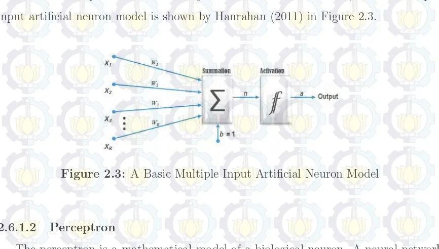
The neuron has a bias b, and the sum of the weighted inputs and the bias forms the net inputn, proceeds into an activation function f, and produces the scalar neuron output (Hagan, Demuth, Beale, and Jesus, 1996). The inputs to a neuron include its bias and the sum of its weighted inputs (using the inner product). The output of a neuron depends on the neurons inputs and on its activation function. This expression can be written as

a=f(W _∗x+b) (2.45)

(37)

the summation represents the cell body and the activation function, a basic multiple-input artificial neuron model is shown by Hanrahan (2011) in Figure 2.3.

Figure 2.3: A Basic Multiple Input Artificial Neuron Model

2.6.1.2 Perceptron

The perceptron is a mathematical model of a biological neuron. A neural network which is made of R input units and one output unit is called a perceptron (Peretto, 1992). Multiplying each input value by a value called the weight is also modeled in the perceptron. The perceptron learning model can be represented as a processing node that receives a number of inputs, forms their weighted sum, and gives an output that is a function of this sum (Dunne, 2007). Perceptrons are useful as classifiers. They can classify linearly separable input vectors very well.

2.6.1.3 Layer

(38)

2.6.2 Radial Basis Function (RBF) Neural Network

Radial functions are simply a class of functions. In principles they could be em-ployed in any sort of model linear or nonlinear and any sort of network single layer or multilayer. The Radial Basis Function Neural Network has local generalization abilities and fast convergence speed (Zhu et al., 2014). Radial basis function neural network consists of input, hidden layer and output. The input contains units of signal source and the output which reacts to input model. The number of units on the hidden layer is determined by K-mean cluster. The movement from input to hidden layer is non-linear and that from hidden layer to output is non-linear. Activation function of the units in hidden layer is Gaussian function.

2.6.2.1 _K-Mean Cluster

RBF centers may be obtained with a clustering procedure such as the K-means algorithm. The real positive numbers (spread) parameters can be computed from the sample covariance of of each cluster. The K-means clustering algorithm starts by picking the numberK of centers and randomly assigning the data points toK subsets. It then uses a simple re-estimation procedure to end up with a partition of the data points intoK disjoint subsets or clusters. These clusters can be used as nodes in Radial Basis Function neural network. The following are K-means algorithm (Johnson and Winchern, 2007)

1. Initialize the clusters center

2. Finding the nearest mean to each data point, reassigning the data points to the associated clusters and then recomputing the new cluster means

3. Repeat step 2 until the old value of old cluster center equal to the value of new cluster center.

2.6.2.2 Radial Functions

(39)

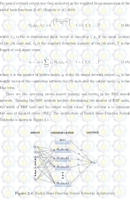
the neural network output was then evaluated as the weighted linear summation of the radial basis functions (2.47) (Kagoda et al., 2010)

Ωj,t(µj, σj) = e −



kxi,t−µjk 2

2σ2 j





,xxt = 1,2,3, . . . , T. (2.46)

where xi,t is the m dimensional input vector at time-step t, µj is the mean (center) of the jth node and, σj is the standard deviation (spread) of the jth node, T is the

length of each input series.

at=ωb +

n X

j=1

ωj.Ωj,t(µj, σj),xxt = 1,2,3, . . . , T. (2.47)

where n is the number of hidden nodes, yt is the ith neural network output, ωj is the weight vector of the connection between the jth node and the output node, ωb is the

bias term.

There are two operating modes named training and testing in the RBF neural network. Training the RBF network involves determining the number of RBF units, the width of RBF units and the output weight values. The criterion is to minimize the sum of squared errors (SSE). The architecture of Radial Basis Function Neural Networks is shown in Figure 2.4.

(40)

The algorithm for Radial Basis Function Neural Network can be derived as follow: 1. Determine the number of clusters by using K-means cluster

2. Compute the values of µj and σj for each input variables within each cluster 3. Compute the values of Ωj,t(µj, σj) in hidden layer unit, e.g. Ω1,1(µ1, σ1) is the

value for the first input in the first node 4. Estimate the weights as the following way:

Consider the network output

a(xi)_≈ω1Ω1,t(µ1, σ1) +· · ·+ωnΩn,t(µn, σn),

we want to find di =a(xi) for each observation, so that

di _≈ω1Ω1,t(µ1, σ1) +· · ·+ωnΩn,t(µn, σn),

in the matrix form, it can be written as

(41)

Finally, the weights can be computed by using the following formula

For example, we will compute RBF neural network by using the residual data from Transfer Function-noise of outflow Lhokseumawe. Suppose our RBF neural network architecture has two inputs at−1 and at−2, one output at, and 2 hidden nodes. These

two hidden nodes are computed by using K-means cluster, the means and standard deviations for every inputs at−1 and at−2 within each node (cluster). Thus by

mini-mizing sum square error, we obtain the weightsω1 =₋30.98, ω2 = 82.75, and the bias

ωb = ₋35.16. Suppose we only compute the forecast for in-sample in this example, then we formulate the RBF neural network model as follow

(42)

the one step ahead forecast can be written as

and if the last two observations we seen from the actual series are at = 4.87 and at−1 = 14.51, the one step ahead forecast output from (2.49) is

2.7 Hybrid Transfer Function - Neural Network Model

Transfer Function and Radial Basis Function Neural Network models have the ad-vantages in their own linear or non linear patterns. However, not all time series types are universally suitable for each of them separately. The reason is, the phenomena of both linear and non linear correlation structures are often occurred among the observa-tions in real world time series. Hence, it is not appropriate to apply Transfer Function and Neural Network models separately to any type of time series data. Therefore a number of efforts are developed to improve time series forecasting methods.

(43)

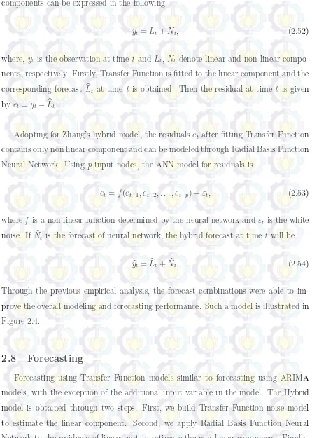
components can be expressed in the following

yt =Lt+Nt, (2.52)

where,yt is the observation at time t and Lt,Nt denote linear and non linear compo-nents, respectively. Firstly, Transfer Function is fitted to the linear component and the corresponding forecast Ltb at time t is obtained. Then the residual at time t is given byet =yt−Lbt.

Adopting for Zhang’s hybrid model, the residualset after fitting Transfer Function

contains only non linear component and can be modeled through Radial Basis Function Neural Network. Usingp input nodes, the ANN model for residuals is

et=f(et−1, et−2, . . . , et−p) +εt, (2.53)

wheref is a non linear function determined by the neural network and εt is the white noise. IfNtb is the forecast of neural network, the hybrid forecast at time t will be

b

yt =Ltb +Nt.b (2.54)

Through the previous empirical analysis, the forecast combinations were able to im-prove the overall modeling and forecasting performance. Such a model is illustrated in Figure 2.4.

2.8 Forecasting

(44)

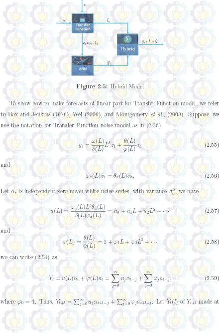
Figure 2.5: Hybrid Model

To show how to make forecasts of linear part for Transfer Function model, we refer to Box and Jenkins (1976), Wei (2006), and Montgomery et al., (2008). Suppose, we use the notation for Transfer Function-noise model as in (2.36)

yt= ω(L) Letαt is independent zero mean white noise series, with varianceσ2

α, we have

we can write (2.54) as

(45)

origin t be the l-step ahead optimal forecast, which is written in the form

Then the forecast error is

Yt+l₋Ytb(l) =

which is minimized if u∗

l+j −ul+j and ϕ ∗

l+j −ϕl+j. Therefore the mean square error

forecast Ytb(l) ofYt+l at origin t is given by the conditional expectation of Yt+l at time

t. Since E[Yt+l₋Ytb(l)] = 0 then the forecast is unbiased. The variance of the lead-l

To make the forecast of non linear part, the residuals from the Transfer Function-noise model is modeled by Radial Basis Function Neural Network. Suppose this pre-diction is obtained as follow

b

Nt=f(et−1, et−2, . . . , et−p) +εt (2.64)

(46)

for both one step ahead and multi step ahead predictions

There are a number of error statistics are used in evaluating forecasting perfor-mance. Here in this research, we only use Root Mean Squared Error (RMSE) and Mean Absolute Deviation (MAD). These methods provide enough information to eval-uate the forecasting performance.

1. Root Mean Squared Error (RMSE)

RM SE =

where the error is calculated as the difference between the target output yt and the network outputy_bt.

2. Mean Absolute Deviation (MAD)

M AD= 1

Linear models have been the focus of theoretical and applied econometrics. Under the stimulus of the economic theory, the relationships between variables of nonlinear models are frequently suggested. Consequently, the interest in testing whether or not a single economic series or group of series may be generated by a nonlinear model against the alternative that they were linearly related instead.

(47)

But here in this study we only use White and Terasvirta tests to detect whether or not a time series data is generated by nonlinear process.

Theorem: Let the Reduced Model is defined as

Yt =f Xt,w_bn(R)+εRt

, (2.68)

where IR is the number of parameters to be estimated. And, let the Full Model that is more complex than the Reduced Model is defined as

Yt=f Xt,w_b_n(F)+εF_t , (2.69)

where IF is the number of parameters in the Full Model, IF > IR . Then, under the hypothesis testing for an additional parameters in the Full Model equal to zero, theF

statistic can be constructed, i.e.

SSE(R)₋SSE(F)/(IF ₋IR)

SSE(F)/(n₋IF) ∼F(v1=[IF−IR],v2=[n−IF]). (2.70)

F test in (2.66) can be written as

F = SSE(R)−SSE(F)/(df(R)−df(F))

SSE(F)/df(F) , (2.71)

or

F = R

2

incremental/(df(R)−df(R))

(1₋R2

(F))/df(F)

, (2.72)

whereR2

incremental =R2(F)−R2(R),df(R)=n−IRis degree of freedom at Reduced Model,

and df(F) =n₋IF is degree of freedom at Full Model.

Generally, Suhartono (2008) define the hypothesis tests which is used in nonliearity test as follow:

(48)

By using F test in (2.71), if the p-value less than α=5%, then the appropriate model to describe the relationship between x and f(x) is nonlinear model.

2.11 Calendar Variation Model

One of the effectiveness model for estimating trading day and moving holiday ef-fects in economic time series is calender variation model. Monthly time series data are frequently subject to calendar variation. In most Islamic countries for example, monthly time series data subject to Ramadhan and Idul Fitri Day effects. A number of calendar variation effect on time series data have been studied by many researchers. Liu (1980) for instance, he studied the effect of holiday variation on the identification and estimation of ARIMA models. Cleveland and Devlin (1980) proposed two sets of diagnostic methods for detecting calendar effects in monthly time series, i.e. by using spectrum analysis and time domain graphical displays. Suhartono, Lee, and Hamzah (2010) developed a calendar variation model based on time series regression method for forecasting time series data with Ramadhan effect. The results show that modeling some real data with calendar variation effect provided better forecast.

Data with calendar variation can also be modeled by using regression (Suhartono, Lee, and Hamzah 2010). Linear regression model for data with calendar variation can be expressed as:

yt =β0+β1V1,t+β2V2,t+_{· · ·}+βpVp,t+wt (2.73) where Vp,t is dummy variable for p-th calendar variation effect, and wt is the error component, usually assumed independently and identically distributed as normal with mean 0 and variance σ2

w. This method can be applied to the identification of

(49)

CHAPTER 3 METHODOLOGY

xxxIn this chapter, we discuss data gathering method and data variables. Indone-sian central bank (BI) of Aceh’s representative offices are located in Banda Aceh and Lhokseumawe. The map of these locations are shown in Figure 3.1.

Figure 3.1: Representative Offices of Indonesian Central Bank (BI) in Aceh Province

3.1 Data and Variables

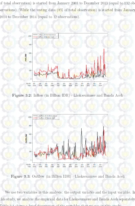
The data set that we use in this analysis is based on monthly data of cash inflow and outflow of Indonesian central bank (BI) at representative offices in Banda Aceh and Lhokseumawe, province of Aceh, Indonesia. We analyzed this monthly data for the periods of time from January 2003 to December 2014. The structure of data consist of inflow, outflow and Consumer Price Index (CPI) with 144 observations and the starting date is at 01.01.2003. Figures 3.2, 3.3, 3.4 show data Inflow, outflow, and Consumer Price Index (CPI) respectively.

(50)

of total observation) is started from January 2003 to December 2013 (equal to 132 ob-servations). While the testing data (8% of total observation) is started from January 2014 to December 2014 (equal to 12 observations).

Figure 3.2: Inflow (in Billion IDR) - Lhokseumawe and Banda Aceh

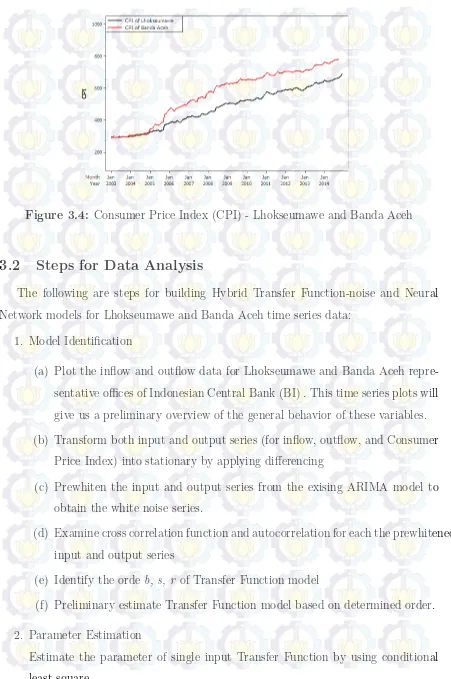
Figure 3.3: Outflow (in Billion IDR) - Lhokseumawe and Banda Aceh

(51)

Figure 3.4: Consumer Price Index (CPI) - Lhokseumawe and Banda Aceh

3.2 Steps for Data Analysis

The following are steps for building Hybrid Transfer Function-noise and Neural Network models for Lhokseumawe and Banda Aceh time series data:

1. Model Identification

(a) Plot the inflow and outflow data for Lhokseumawe and Banda Aceh repre-sentative offices of Indonesian Central Bank (BI) . This time series plots will give us a preliminary overview of the general behavior of these variables. (b) Transform both input and output series (for inflow, outflow, and Consumer

Price Index) into stationary by applying differencing

(c) Prewhiten the input and output series from the exising ARIMA model to obtain the white noise series.

(d) Examine cross correlation function and autocorrelation for each the prewhitened input and output series

(e) Identify the orde b, s, r of Transfer Function model

(f) Preliminary estimate Transfer Function model based on determined order. 2. Parameter Estimation

(52)

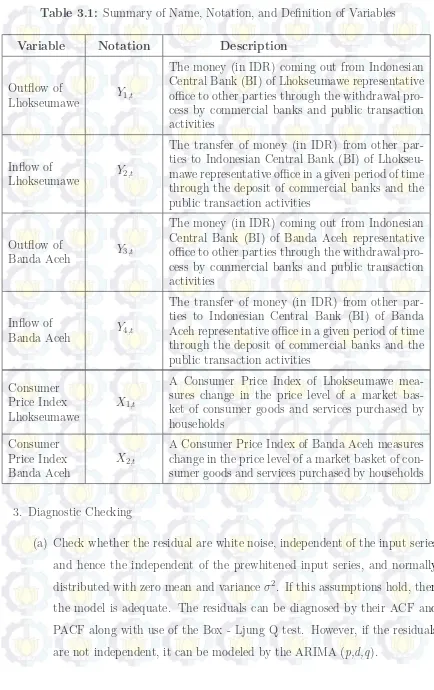
Table 3.1: Summary of Name, Notation, and Definition of Variables

spacyspacyspacyspacyspacyspacyspacyspacyspacyspacyspacy

Variable Notation Description

Outflow of

Lhokseumawe xxxxY1,t

The money (in IDR) coming out from Indonesian Central Bank (BI) of Lhokseumawe representative office to other parties through the withdrawal pro-cess by commercial banks and public transaction activities

Inflow of

Lhokseumawe xxxxY2,t

The transfer of money (in IDR) from other par-ties to Indonesian Central Bank (BI) of Lhokseu-mawe representative office in a given period of time through the deposit of commercial banks and the public transaction activities

Outflow of

Banda Aceh xxxxY3,t

The money (in IDR) coming out from Indonesian Central Bank (BI) of Banda Aceh representative office to other parties through the withdrawal pro-cess by commercial banks and public transaction activities

Inflow of

Banda Aceh xxxxY4,t

The transfer of money (in IDR) from other par-ties to Indonesian Central Bank (BI) of Banda Aceh representative office in a given period of time through the deposit of commercial banks and the public transaction activities

Consumer Price Index Lhokseumawe

xxxxX1,t

A Consumer Price Index of Lhokseumawe mea-sures change in the price level of a market bas-ket of consumer goods and services purchased by households

Consumer Price Index Banda Aceh

xxxxX2,t

A Consumer Price Index of Banda Aceh measures change in the price level of a market basket of con-sumer goods and services purchased by households

3. Diagnostic Checking

(a) Check whether the residual are white noise, independent of the input series and hence the independent of the prewhitened input series, and normally distributed with zero mean and variance σ2_{. If this assumptions hold, then}

(53)

(b) After obtaining the predictions from Transfer Function-noise model, the residual series is used to model the Radial Basis Function Neural Network. 4. Forecasting

(a) Compute the residual from Transfer Function-noise model et=yt₋Ltb

(b) Forecast the pure linear part of Transfer Function model (c) Forecast the non linear part of Neural Network model

(54)

(55)

CHAPTER 4 RESULTS AND ANALYSIS

xxxSix data sets are used in this research. These six sets of time series data are shown in Figure 3.2, Figure 3.3, and Figure 3.4. We see that the series Inflow, Outflow, and con-sumer price index (CPI) in Banda Aceh and Lhokseumawe are clearly non-stationary series, they are trending up over the given time period. Therefore, differencing is re-quired to obtain stationarity. In this study we use a single input and single output models.

The general steps of Transfer Function-noise model building process is applied to obtained the appropriate linear model. After obtaining the predictions of Transfer Function-noise model, its residual series is used to form non linear model by using the Radial Basis Function (RBF) Neural Network. We estimated several different RBF Neural network models with different nodes in training data (in-sample) in order to obtain the optimum networks. It is aimed to better capture the underlying behavior of the time series movement of Inflow and Outflow for both Lhokseumawe and Banda Aceh representative offices.

We use single layer network with 2 input and 1 output for model building process of the entire series in this research. 5 node is the most optimum network in comparison to the other tested nodes of the residuals of Lhokseumawe Outflow and 10 node is for the residual of Lhokseumawe Inflow series. While the optimum network of residual series of Outflow Banda Aceh is 8 node. The network of residual Inflow Banda Aceh residual is optimized in 25 nodes. Nodes are computed by using K-means cluster. Means and standard deviations are computed for each input variables within each nodes. In hidden layer, bias term is employed and the Gaussian function is used as the activation function for each nodes.

(56)

represents a set of true “unseen future” observations for testing the proposed model effectiveness as well as for model comparisons.

Prior to apply the Neural Network and Hybrid model, we first test the residual of Transfer Function-noise model by using the White and Terasvirta tests. Table 4.1 show that all data have the nonlinear relationship between residual and its first and second lags, except for residual of Inflow Banda Aceh, where bothp-values of White test and Terasvirta test are larger than α=5%. In this study, we use several software packages

Table 4.1: Nonliearity Test

spacy

Residual P-value of White Test P-value of Terasvirta Test

Outflow Lhokseumawe 0.081 0.036

Inflow Lhokseumawe 0.002 0.002

Outflow Banda Aceh 9.004e-14 2.442e-15

Inflow Banda Aceh 0.305 0.385

to run the data. All Transfer Function-noise modeling is implemented via SAS system while neural network models are built using Matlab. Non linearity test is performed by R. All figures are plotted by Minitab. The Root Mean Squared Error (MSE) and Mean Absolute Deviation (MAD) are selected to be the forecasting accuracy measures.

4.1 Lhokseumawe Representative Office

4.1.1 Outflow of Lhokseumawe

(57)

sample cross correlation of the prewhitened input αt and the prewhitened output βt. The crosscorrelation function (CCF) betweenαt andβt is given in Appendix A.3. The

(a) 1st

Differencing

(b) ACF (c) PACF

Figure 4.1: Time Series plots of Differenced CPI, ACF, and PACF of Lhokseumawe

CCF output indicate that there is a delay of 0 lag in the system, then we specify b = 0. The specifications of the orderss and r are based on the number of spikes in CCF after 0 lag. There are several spikes appear after lag 0, but only lag 1 are significant, then we specify the order of s is subset 1 and we set the denominator as zero, that is,

r=0. Now we fit the noise which incorporate into the overall model. From the output in Appendix A.4 and Appendix A.5, the subset ARIMA([1,2,12],0,[3,23]) is the most parsimony model for noise term. The appropriate coefficients estimation areω0 = 5.55,

(58)

yt= (ω0₋ω1L1)xt+ 1−θ3L

Next step is to forecast the Transfer Function-noise model in (4.1). The residualat

is analyzed by using Radial Basis Function Neural Network. The nonlinearity test in Table 4.1 indicate a non linear relationship between the residual of Outflow Lhokseu-mawe series and its first and second lags. The optimal estimated weights of this model are ω1 = −30.98, ω2 = 82.75, ω3 = −339.45, ω4 = 38.23, ω5 = −12.43, and the bias

and µ, σ for each node (cluster) are availiable in Appendix C.1.

(59)

RMSE and MAD respectively

Table 4.2: Measurement of Performance Test for Outflow Series of Lhokseumawe

Model In-Sample Out-Sample

xxRMSExx xxMADxx xxRMSExx xxMADxx

TF-ARIMA NOISE 106.19 73.42 106.76 79.14

HYBRID 102.91 72.97 112.53 82.70

Figures 4.2 and Figures 4.3 show the comparison between actual observations and the forecasts from the in-sample and out-sample horizons of Transfer Function-noise model and Hybrid model of Lhokseumawe Outflow series respectively.

(a) In-sample (b) Out-sample

Figure 4.2: Actual vs Transfer Function-Noise prediction of Outflow Lhokseumawe

(60)

4.1.2 Inflow of Lhokseumawe

In a similar fashion to the Outflow series, we first fit an ARIMA model to the Consumer Price Index (CPI) of Lhokseumawe. The first differencing of this series is shown in Figure 4.1(a). The ACF and PACF plots in Figure 4.1(b) and Figure 4.1(c) indicate that the subset ARIMA([1,2,8],1,0) is appropriate to model Consumer Price Index (CPI) series. This model is used as a filter to prewhiten the input and the output series.

The CCF output (Appendix A.9) indicate that there is a delay of 1 lag in the system, then we specify b = 1. The specifications of the orders s and r are based on the number of spikes in CCF after 1 lag. There are several spikes appear after lag 1. In identification step, we found that there are two possible candidate Transfer Function-noise model for Inflow series.

The first model, we identify the orders of b=1, the subset s=[1,5,6,10,11] and r=0. The noise model is identified to be ARIMA(0,0,0). The appropriate coefficients esti-mation are ω0 = 1.91, ω1 = 2.44, ω5 = 1.69, ω6 =−2.03, ω10 = 1.81, ω11 =−1.83. All

these parameters are significant. Thus the Transfer Function-noise model is given as follow

yt= (ω0₋ω1L₋ω5L5 ₋ω6L6 ₋ω10L10₋ω11L11)L1xt+at

= (1.91₋2.44L₋1.69L5+ 2.03L6₋1.81L10+ 1.83L11)xt−1+at.

(4.3)

The second model, the orders ofb, s, andr are identified to be equal to zero. While the noise model is fit to follow the subset ARIMA(12,0,[1,22,23,24]). The appropriate coefficients estimation are ω0 = 0.78, θ1 = 0.73, θ22 = 0.29, θ23 = ₋0.64, θ24 = 0.31,

ϕ12 = 0.48. Thus the Transfer Function-noise model is given as follow

yt=ω0xt+ 1−θ1L−θ22L

22₋_θ23L23₋_θ24L24

1₋ϕ12L12 at

= 0.78xt+

1₋0.73L₋0.29L22_{+ 0}_.₆₄_L23₋₀_.₃₁_L24

1₋0.48L12 at

(4.4)

(61)

Base on this reason, we choose model 1 to proceed to Neural Network forecasting. The parameters estimation of model 1 is given in Appendix A.8. Since all coefficients are less than α= 10%, these parameters are significant.

Next step is to forecast the Transfer Function-noise of model 1 (4.3). The residual

atis analyzed by using Radial Basis Function Neural Network. Table 4.1 indicate a non linear relationship between the residual of Inflow Lhokseumawe series and its first and second lags. The optimal estimated weights of Inflow series model are ω1 = ₋32.56,

ω2 = 91.42, ω3 = 102.12, ω4 = ₋377.96, ω5 = 139.86, ω6 = ₋133.99, ω7 = 50.37,

(62)

Table 4.3: Measurement of Performance Test for Inflow Series of Lhokseumawe

TF-ARIMA NOISE 61.81 39.17 165.47 73.47

HYBRID 50.51 32.66 168.94 91.48

Figures 4.4 and Figures 4.5 show the comparison between actual observations and the forecasts from the in-sample and out-sample horizons of Transfer Function-noise model 1 and Hybrid model 1 of Lhokseumawe Inflow series respectively.

Figure 4.4: Actual vs Transfer Function-Noise prediction of Inflow Lhokseumawe-Model 1

(63)

4.2 Banda Aceh Representative Office

4.2.1 Outflow of Banda Aceh

We first prewhiten the Consumer Price Index (CPI) series of Banda Aceh. The original series of Banda Aceh CPI series is not stationary, but its difference is assumed to be stationary (Figure 4.6.a). By examining the sample ACF and PACF in Figure 4.6(b) and Figure 4.6(c), the time series plot suggest that the subset ARIMA([6],1,0) is appropriate to prewhiten input series as well as the output series of Banda Aceh.

(a) 1st

Differencing

(b) ACF (c) PACF

Figure 4.6: Time Series plots of Differenced CPI, ACF, and PACF of Banda Aceh

The sample CCF output (Appendix B.3) suggest the order of b=1, r=0, and s=0. The noise model from overall model (Appendix B.4 and Appendix B.5) is identified to follow the ARIMA(0,0,0). The significant estimated coefficients (all coefficients are less than α = 10%) of this model is ω0 = ₋4.89 (Appendix B.2). Thus the model is given as follow

yt=ω0L1xt+at

=₋4.89Xt−1+at

(64)

Next step is to forecast the Transfer Function-noise model in (4.6). The residualat

is modeled by using Radial Basis Function Neural Network. This analysis is conducted due to non linear relationship between residual of Outflow Banda Aceh and its first and second lags as indicated in Table 4.1. The optimal estimated weights of Inflow series model are ω1 = 70.59, ω2 = 0.0001, ω3 = 108.39, ω4 = ₋128.19, ω5 = ₋4.50,

ω6 = 162.31, ω7 = 63.41, ω8 = 4.93, and the bias weight ωb = ₋4.29. Thus, RBF neural network model fora(t) is as follow

a(t) =

and µ, σ for each node (cluster) are available in Appendix C.3.

(65)

Table 4.4: Measurement of Performance Test for Outflow Series of Banda Aceh

TF-ARIMA NOISE 170.30 120.38 510.24 460.80

HYBRID 160.14 115.09 514.71 465.07

Figure 4.7: Actual vs Transfer Function-Noise prediction of Outflow Banda Aceh

Figure 4.8: Actual vs Hybrid prediction of Outflow Banda Aceh

4.2.2 Inflow of Banda Aceh

(66)

and output series. The CCF between αt and βt is given in Appendix B.6.

The CCF output indicate that there is a delay of 1 lag in the system (Appendix B.9), then we specify b = 1. There are several spikes appear after lag 1, we specify the order of s are subset 2 and we set the denominator as zero, that is, r=0. From the output in Appendix B.10 and Appendix B.11, the subset ARIMA(0,0,[1,12,13]) is the most parsimony model for noise term. The appropriate significant coefficients estimation areω0 = 1.13, ω2 = 1.03, θ1 = 0.51, θ12 =₋0.46, andθ13= 0.49 (Appendix B.8). These coefficients are significant since they are less than α = 10%. Thus the Transfer Function-noise model for Inflow series of Banda Aceh is given as follow:

yt= (ω0₋ω2L2)L1xt+ (1₋θ1L₋θ12L12₋θ13L13)at

= (1.13₋1.03L2)xt−1+ (1−0.51L+ 0.46L12−0.49L13)at

(4.8)

Next step is to forecast the Transfer Function-noise model in (4.8). The relationship of residual of Inflow Banda Aceh with its first and second lags is not nonlinear (Table 4.1). The residual at is modeled by using Radial Basis Function Neural Network. The

optimal estimated weights of Inflow Banda Aceh series model are ω1 = 11.64, ω2 =

(67)

Ω25,t(µ25, σ25) = exp

−1 2

_at− 1−µ251 σ251

2

+at−2−µ252 σ252

2

,

xx

Table 4.5 shows that the Root Mean Square Error (RMSE) and the Mean Absolute Deviation of in-sample hybrid model can be slightly reduced by 4.19% and 3.71% respectively. However, RMSE and MAD slightly rise by 1.34% and 0.79% respectively. It is no surprise since the relationship of Inflow Banda Aceh residual and its first and second lags doesn’t indicate the nonlinear relationship. Figures 4.9 and Figures 4.10

Table 4.5: Measurement of Performance Test for Outflow Series of Banda Aceh

TF-ARIMA NOISE 66.75 47.13 142.13 104.15

HYBRID 65.95 45.38 144.04 104.97

show the comparison between actual observations and the forecasts from the in-sample and out-sample horizons of Transfer Function-noise model and Hybrid model of Banda Aceh Inflow series respectively.

(68)

Figure 4.10: Actual vs Hybrid prediction of Inflow Banda Aceh

4.2.3 Calendar Variation

The main objective of outflow and inflow modeling is ultimately to predict the direction and level of change in a given series. However, this financial series are quanti-tative measures of given behavior of underlying factors (holiday, consumers, businesses, traders, etc.). Given that the behavior of economic factors, the four hybrid model we have developed do not show the superior models in out-sample. This poor forecasts may probably affected by local and national condition in Aceh and Indonesia in a cer-tain months, particularly during June to August of 2014. For instance, the Idul Fitri day fell in July in the year of 2014. In this period, the money coming out/in from/to Bank Indonesia is irregularly different from the normal daily activities.

A HYBRID TRANSFER FUNCTION AND ARTIFICIAL NEURAL NETWORK MODEL FOR TIME SERIES FORECASTING - ITS Repository