Title An artificial bee colony algorithm for the capacitatedvehicle routing problem
Author(s) Szeto, WY; Wu, Y; Ho, SC
Citation European Journal Of Operational Research, 2011, v. 215n. 1, p. 126-135
Issue Date 2011
URL http://hdl.handle.net/10722/135063
Rights
NOTICE: this is the author’s version of a work that was accepted for publication in European Journal of
Operational Research. Changes resulting from the publishing process, such as peer review, editing,
corrections, structural formatting, and other quality control mechanisms may not be reflected in this document. Changes may have been made to this work since it was submitted for publication. A definitive version was
1
An Artificial Bee Colony Algorithm for the Capacitated
Vehicle Routing Problem
W. Y. Szeto1,2, Yongzhong Wu3 and Sin C. Ho4
2 Department of Civil Engineering, The University of Hong Kong, Pokfulam Road, Hong Kong, PR China
3 Department of Industrial Engineering, South China University of Technology, PR China 4 CORAL, Department of Business Studies, School of Business and Social Sciences,
Aarhus University, Denmark
Abstract
This paper introduces an artificial bee colony heuristic for solving the capacitated vehicle routing problem. The artificial bee colony heuristic is a swarm-based heuristic, which mimics the foraging behavior of a honey bee swarm. An enhanced version of the artificial bee colony heuristic is also proposed to improve the solution quality of the original version. The performance of the enhanced heuristic is evaluated on two sets of standard benchmark instances, and compared with the original artificial bee colony heuristic. The computational results show that the enhanced heuristic outperforms the original one, and can produce good solutions when compared with the existing heuristics. These results seem to indicate that the enhanced heuristic is an alternative to solve the capacitated vehicle routing problem.
Keywords: Routing, Artificial Bee Colony, Metaheuristic
2 1. Introduction
The Capacitated Vehicle Routing Problem (CVRP) (i.e., the classical vehicle routing problem) is defined on a complete undirected graph G=( , )V E , where V ={0,1, , }… n is the vertex set and
( )
{ , : , , }
E= i j i j∈V i< j is the edge set. Vertices 1, ,… n represent customers; each customer i is associated with a nonnegative demand di and a nonnegative service time si. Vertex 0 represents
the depot at which a fleet of m homogeneous vehicles of capacity Q is based. The fleet size is
treated as a decision variable. Each edge ( , )i j is associated a nonnegative traveling cost or travel
time cij. The CVRP is to determine m vehicle routes such that (a) every route starts and ends at the
depot; (b) every customer is visited exactly once; (c) the total demand of any vehicle route does not exceed Q; and (d) the total cost of all vehicle routes is minimized. In some cases, the CVRP also
imposes duration constraints where the duration of any vehicle route must not exceed a given bound
L. Mathematical formulations of the CVRP can be found in Toth and Vigo (2002).
As the CVRP is a NP-hard problem, only instances of small sizes can be solved to optimality using exact solution methods (e.g., Toth and Vigo, 2002; Baldacci et al., 2010), and this might not even be possible if it is required to use limited amount of computing time. As a result of this, heuristic methods are used to find good, but not necessarily guaranteed optimal solutions using reasonable amount of computing time. During the past two decades, an increasing number of publications on heuristic approaches have been developed to tackle the CVRP. The work can be categorized into evolutionary algorithms (Baker and Ayechew, 2003; Berger and Barkaoui, 2003; Prins, 2004; Mester and Bräysy, 2007; Prins, 2009; Nagata and Bräysy, 2009), ant colony optimization (Bullnheimer et al., 1999; Reimann et al., 2004; Yu et al., 2009), simulated annealing (Osman, 1993; Lin et al., 2009), tabu search (Taillard, 1993; Gendreau et al., 1994; Rego and Roucairol, 1996; Rego, 1998; Cordeau et al., 2001; Toth and Vigo, 2003; Derigs and Kaiser, 2007), path-relinking (Ho and Gendreau, 2006), adaptive memory procedures (Rochat and Taillard, 1995; Tarantilis and Kiranoudis, 2002; Tarantilis, 2005), large neighborhood search (Ergun et al., 2006; Pisinger and Ropke, 2007), variable neighborhood search (Kytöjoki et al., 2007; Chen et al., 2010), deterministic annealing (Golden et al., 1998; Li et al., 2005), honey-bees mating optimization (Marinakis et al., 2010), particle swarm optimization (Ai and Kachitvichyanukul, 2009) and hybrid Clarke and Wright’s savings heuristic (Juan et al., 2010).
3
procedure used the idea of genetic algorithms of combining solutions to construct new solutions and employed the tabu search of Taillard (1993) as an improvement procedure. Tarantilis (2005) had a similar framework as Tarantilis and Kiranoudis (2002) (which is a variant of the idea proposed by Rochat and Taillard), but is different in that it does not rely on probability as in Tarantilis and Kiranoudis (2002) and also uses a more sophisticated improvement procedure. The Unified tabu
search (Cordeau et al., 2001) and the tabu search used by Ho and Gendreau (2006) contain some of
the features found in Taburoute (Gendreau et al., 1994); infeasible solutions are considered by extending the objective function with a penalty function and the use of continuous diversification.
Granular tabu search (Toth and Vigo, 2003) restricts the neighborhood size by removing edges
from the graph that are unlikely to appear in an optimal solution. Later, other researchers have also applied this idea on their CVRP heuristics (e.g., Li et al., 2005; Mester and Bräysy, 2007; Chen et al., 2010). For extensive surveys on VRP metaheuristics, the reader is referred to Gendreau et al. (2002), Cordeau et al. (2005) and Gendreau et al. (2008).
While the above heuristics have been widely used and successfully applied to solve the CVRP for several years, Artificial Bee Colony (ABC) is a fairly new approach introduced just a few years ago by Karaboga (2005), but has not yet been applied to solve the CVRP. However, ABC has been applied to solve other problems with great success (Baykasoğly et al., 2007; Kang et al., 2009;
Karaboga, 2009; Karaboga and Basturk, 2007, 2008; Karaboga and Ozturk, 2009; Singh, 2009). It is worthwhile to evaluate the performance of the ABC algorithm for solving the CVRP.
4 2. Artificial bee colony algorithm
The ABC algorithm belongs to a class of evolutionary algorithms that are inspired by the intelligent behavior of the honey bees in finding nectar sources around their hives. This class of metaheuristics has only started to receive attention recently. Different variations of bee algorithms under various names have been proposed to solve combinatorial problems. But in all of them, some common search strategies are applied; that is, complete or partial solutions are considered as food sources and the groups of bees try to exploit the food sources in the hope of finding good quality nectar (i.e., high quality solutions) for the hive. In addition, bees communicate between themselves about the search space and the food sources by performing a waggle dance.
In the ABC algorithm, the bees are divided into three types; employed bees, onlookers and scouts. Employed bees are responsible for exploiting available food sources and gathering required information. They also share the information with the onlookers, and the onlookers select existing food sources to be further explored. When the food source is abandoned by its employed bee, the employed bee becomes a scout and starts to search for a new food source in the vicinity of the hive. The abandonment happens when the quality of the food source is not improved after performing a maximum allowable number of iterations.
5
is assigned to a food source, another iteration of the ABC algorithm begins. The whole process is repeated until a stopping condition is met.
The steps of the ABC algorithm are summarized as follows:
1. Randomly generate a set of solutions as initial food sources xi, i= …1, ,τ . Assign each
employed bee to a food source.
2. Evaluate the fitness ( )f xi of each of the food sources xi, i= …1, ,τ .
3. Set v=0 and l1= = … = =l2 lτ 0.
4. Repeat
a.For each food source xi
i. Apply a neighborhood operator on xi →xɶ.
ii. If f
( )
xɶ > f( )xi , then replace xi with xɶ and li =0, else li = +li 1.b.Set Gi = ∅ = …, i 1, ,τ , where Gi is the set of neighbor solutions of food source i.
c.For each onlooker
i. Select a food source xi using the fitness-based roulette wheel selection
method.
ii. Apply a neighborhood operator on xi →xɶ.
iii. Gi =Gi∪{ }xɶ
d.For each food source xi and Gi ≠ ∅
i. Set ˆ arg max ( )
i
G
x∈ σ∈ f σ .
ii. If f x
( )
i < f( )
xˆ , then replace xi with ˆx and li =0, else li = +li 1.e.For each food source xi
i. If li =limit, then replace xi with a randomly generated solution.
f. v= +v 1
5. Until (v=MaxIterations)
3. Application to the CVRP
6 3.1 Solution representation
In order to maintain the simplicity of the ABC algorithm, a rather straightforward solution representation scheme is adopted. Suppose n customers are visited by m vehicle routes. The representation has the form of a vector of length (n+m). In the vector, there are n integers
between 1 and n inclusively representing customers’ identity. There are also m 0s in the vector representing the start of each vehicle route from the depot. The sequence between two 0s is the sequence of customers to be visited by a vehicle. Figure 1 illustrates a representation of a CVRP instance with n=7 and m=3. As shown in Figure 1, customers 4 and 1 are assigned to the same
vehicle route and the vehicle visits customer 4 before customer 1.
Figure 1. Solution representation
3.2 Search space and cost functions
The search may become restrictive if only the feasible part of the solution space is explored. Hence, we also allow the search to be conducted in the infeasible part of the solution space, so that the search can oscillate between feasible and infeasible parts of the solution space X . Each solution
x∈X consists of m vehicle routes where each one of them starts and ends at the depot, and every
customer is visited exactly once. Thus, x may be infeasible with regard to the capacity and/or
duration constraints. For a solution x, let ( )c x denote its travel cost, and let ( )q x and ( )t x denote
the total violation of the capacity and duration constraints respectively. The routing cost of a vehicle
k corresponds to the sum of the costs cij associated with the edges ( , )i j traversed by this vehicle.
The total violation of the capacity and duration constraints is computed on a route basis with respect to Q and L . Each solution x found in the search is evaluated by a cost function
( ) ( )
( )
( )z x =c x +αq x +βt x that includes the considerations mentioned above. The coefficients α
and β are self-adjusting positive parameters that are modified at every iteration. The parameter α is adjusted as follows: If the number of solutions with no violation of the capacity constraints is greater than / 2τ , the value of α is divided by 1+δ , otherwise it is multiplied by 1+δ. The same rule also applies to β with respect to the duration constraints.
7 3.3 Initial solution
An initial solution is constructed by assigning one customer at a time to one of the m vehicle routes. The selection of the customer is randomly made. The customer is then assigned to the location that minimizes the cost of assigning this customer over the current set of vehicle routes. The above procedure is repeated until all customers are routed.
A total of τ initial solutions are generated by the above procedure.
3.4 Neighborhood operators
A neighborhood operator is used to obtain a new solution xɶ from the current solution x in Step 4 of the ABC heuristic. A number of neighborhood operators (among those listed below) are chosen in advance. Any combinations of the listed operators are possible, even one. Then, whenever a new solution xɶ is needed, a neighborhood operator is randomly chosen from the set of pre-selected neighborhood operators and applied once (i.e., no local search is performed) to the solution x. The set of pre-selected operators is determined by experimental testing discussed in Section 4.1. The possible operators include:
1. Random swaps
This operator randomly selects positions (in the solution vector) i and j with i≠ j and swaps the customers located in positions i and j. See Figure 2, where i=3 and j=7.
Figure 2. Random swaps
2. Random swaps of subsequences
This operator is an extension of the previous one, where two subsequences of customers and depot of random lengths are selected and swapped. An example is shown in Figure 3.
0 4 1 0 2 7 5 0 3 6
0 4 5 0 2 7 1 0 3 6
Before:
After:
8
Figure 3. Random swaps of subsequences
3. Random insertions
This operator consists of randomly selecting positions i and j with i≠ j and relocating the customer from position i to position j. See Figure 4, where customer 5 is relocated from
position 7 to position 3.
Figure 4. Random insertions
4. Random insertions of subsequences
This operator is an extension of the operator of random insertions where a subsequence of customers and depot of random length starting from position i is relocated to position j.
Positions i and j are randomly selected. Figure 5 gives an example of this operator.
Figure 5. Random insertions of subsequences
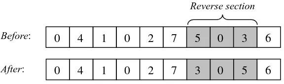
5. Reversing a subsequence
A subsequence of consecutive customers and depot of random length is selected and then the order of the corresponding customers and depot is reversed, as shown in Figure 6.
0 4 1 0 2 7 5 0 3 6
0 4 5 0 3 2 7 1 0 6
Before:
After:
Swap section Swap section
0 4 1 0 2 7 5 0 3 6
0 4 5 0 3 1 0 2 7 6
Before:
After:
Insert position Insert section
0 4 1 0 2 7 5 0 3 6
0 4 5 1 0 2 7 0 3 6
Before:
After:
9
Figure 6. Reversing a subsequence
6. Random swaps of reversed subsequences
This operator is a combination of two previously mentioned operators. Two subsequences of customers and depot of random lengths are chosen and swapped. Then each of the swapped subsequences may be reversed with a probability of 50%. An example of this operator is displayed in Figure 7.
Figure 7. Random swaps of reversed subsequences
7. Random insertions of reversed subsequences
A subsequence of customers and depot of random length starting from position i is relocated to position j. Then the relocated subsequence has a 50% chance of being reversed.
Figure 8 shows an example of this operator where i=7 and j=3, and the subsequence is
reversed.
Figure 8. Random insertions of reversed subsequences
Before:
After:
Reverse section
0 4 1 0 2 7 5 0 3 6
0 4 1 0 2 7 3 0 5 6
Before:
After:
0 4 1 0 2 7 5 0 3 6
0 4 3 0 5 1 0 2 7 6
Insert position Insert-reverse section Before:
After:
0 4 1 0 2 7 5 0 3 6
0 4 3 0 5 2 7 0 1 6
10 3.5 Selection of food sources
At each iteration of the algorithm, each onlooker selects a food source randomly. In order to drive the selection process towards better food sources, we have implemented a roulette-wheel selection
method for randomly selecting a food source. The probability of choosing the food source xi is then
defined as
( )
3.6 An enhanced artificial bee colony algorithm
It is shown in the literature that the basic ABC algorithm is capable of solving certain problems with great success. However, according to our computational experiments (see Section 4) this does not apply to the CVRP. Therefore, in this section, we will propose an enhanced version of the ABC algorithm to improve the performance of the basic ABC algorithm for solving the CVRP.
Step 4d of the basic ABC algorithm states that a food source xi will only be replaced by a neighbor
solution ˆx if ˆx is of a better quality than xi, where ˆx is the best neighbor solution found by the
onlookers in Step 4b. In the refined version, this condition is altered so that if the best neighbor solution ˆx found by all the onlookers associated with food source i is better than the food source
i
x , then ˆx will replace the food source xj that possesses the following two properties: 1) xj has
not been improved for the largest number of iterations among all the existing food sources and 2)
j
x is worse than ˆx. In this way, potential food sources (i.e., the food sources which can produce
better neighbor solutions) will be given opportunities to be further explored whereas non-potential food sources (i.e., the food sources which have not been improved for a relatively large number of iterations and are worse than new neighbor solutions) are excluded.
Step 4e of the basic ABC algorithm states that if no improving neighbor solutions of the food source
i
x have been identified during the last limit successive iterations, then xi is replaced by a
randomly generated solution (using the procedure described in Section 3.3). In the refined version,
this is modified so that xi is replaced by a new neighbor solution ˆx of xi. The quality of ˆx can be
worse or better than xi . This modification may be beneficial as it prevents the search from
searching in bad regions of the solution space with no control of the quality of the food sources.
11
1. Randomly generate a set of solutions as initial food sources xi, i= …1, ,τ .
Set F = ∪τi=1{ }xi , where F is the set of food sources. Assign each employed bee to a food
source.
2. Evaluate the fitness ( )f xi of each of the food sources xi, i= …1, ,τ .
3. Set v=0 and l1= = … = =l2 lτ 0.
4. Repeat
a.For each food source xi
i. Apply a neighborhood operator on xi →xɶ.
ii. If f x
( )
ɶ > f x( )
i , then replace xi with xɶ and li =0, else li = +li 1.b.Set Gi = ∅ = …, i 1, ,τ . c.For each onlooker
i. Select a food source xi using the fitness-based roulette wheel selection
method.
ii. Apply a neighborhood operator on xi →xɶ.
d. Gi =Gi∪{ }xɶ
e.For each food source xi and Gi ≠ ∅
i. Set ˆ arg max ( )
i
G
x∈ σ∈ f σ .
ii. If f x
( )
i < f x( )ˆ , then select xɶj∈F with( )
1, , ˆ
arg maxi F{ | ( )i i and i }
j∈ = … l f x > f x x ∈F , replace xɶj with ˆx, and
0
i
l = , else li = +li 1.
f. For each food source xi
i. If li =limit, then apply a neighborhood operator on xi →xɶ and replace xi
with xɶ.
g. v= +v 1
5. Until (v=MaxIterations)
4. Computational experiments
12
instance sets. These include the fourteen classical Euclidean VRP and distance-constrained VRP instances described in Christofides and Eilon (1969) and Christofides et al. (1979) and the twenty large scale instances described in Golden et al. (1998). All experiments were performed on a 1.73 GHz computer, and the heuristics were coded in Visual C++ 2003.
The number of employed bees and the number of onlookers are set to be equal to the number of food sources (τ ), which is 25. This is based on Karaboga and Basturk (2008), which set the number of employed bees to be equal to the number of onlookers to reduce the number of parameters, and find that the colony size (i.e., the total number of employed bees and onlookers) of 50 can provide an acceptable convergence speed for search.
To reduce the number of parameters tuned, we let α = β. We then evaluated the performance of the heuristics using different values of α in the interval [0.0001, 1] and δ = 0.001. It is found that the performance of the heuristics is insensitive over this range for many test instances, and for a majority of the test instances setting α = β to 0.1 seems to be the best choice. Based on these values of α and β, we tested the best value of δ over the range [0.0001, 1]. The results show that the performance of the heuristics varies significantly in this interval for many test instances, and good solutions are obtained with δ = 0.001. Therefore, we set α = β =0.1 and δ = 0.001 for all further experiments.
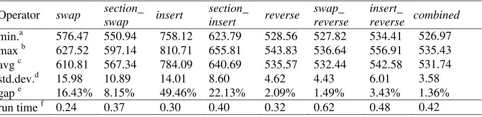
4.1 Comparison of neighborhood operators
In order to evaluate the effectiveness of each neighborhood operator, we have first tested the original ABC heuristic on instance vrpnc1 by considering each neighborhood operator at a time, including: 1. random swaps (swap); 2. random swaps of subsequences (section_swap); 3. random
insertions (insert); 4. random insertions of subsequences (section_insert); 5. reversing a
subsequence (reverse); 6. random swaps of reversed subsequences (swap_reverse); and 7. random
insertions of reversed subsequences (insert_reverse). The results are reported in Table 1. The best
13
reversed subsequences did not lead to the best known solution, the average deviation from the best known solution is less than 1.5%. Reversing a subsequence is another operator which also yields good performance, and uses less computation time than the operator of randomly swapping reversed subsequences.
Table 1. Experimental results by different operators for instance vrpnc1
Operator swap section_
a Minimum objective value obtained in 20 runs b Maximum objective value obtained in 20 runs c Average objective value of 20 runs
d Standard deviation of objective values of 20 runs
e Average percentage deviation from the best known solution f Average CPU time in minutes for each run
The search using only the operator of randomly swapping reversed subsequences may be too diversified, and may not lead to promising regions of the solution space. Thus, instead of using only one operator we will use a combination of several operators. A number of different combinations of operators have been tried and experimented with. The combination of the following operators seems to yield the most promising results: random swaps (swap), reversing a subsequence (reverse) and random swaps of reversed subsequences (swap_reverse). This seems reasonable as two of the operators were identified to yield the best results from Table 1, while the search using the third operator (i.e., random swapping) is not as diversified as the searches using the two other operators. Equal probabilities are associated with the operators being selected. Using this combination of operators, the heuristic was run and obtained an average deviation of 1.36% from the best known solution, as shown in the last column (combined) of Table 1. In addition, it is also faster than the variant using randomly swapping of reversed subsequences (swap_reverse) as the neighborhood operator.
14
subsequences (swap_reverse) and the combination of the operators for randomly swapping two positions, reversing a subsequence, and randomly swapping reversed subsequences (combined) during one run on instance vrpnc1. It can be observed from the figure that the variant using the operator of reversing a subsequence converges faster than the other two. However, the solution quality is not good as reflected by the objective value, which is the highest among the three operators. The operator of randomly swapping reversed subsequences converges at a later stage but achieves a better solution. The combined approach leads to the best solution quality than the other two, and the convergence rate is somewhere between the other two. This phenomenon was also observed when the different variants of the heuristic were experimented on the rest of the test instances. For this reason, the combination of the three different operators will be adopted in the heuristic to generate neighbor solutions.
4.2 Calibrating limit
As mentioned earlier, a food source xi will be abandoned if no improving neighbor solutions xˆ can
be found in the neighborhood of xi for consecutive limit iterations. Karaboga (2009) has shown
that this parameter is important regarding the performance of the ABC algorithm on solving function optimization problems. Hence, we will also study the effect of this parameter on the performance of the ABC algorithm for solving the CVRP.
The value of the parameter limit was determined by running every benchmark instance 20 times for each of the predetermined values of limit. This calibrating process is important because if too few iterations are spent on exploring the neighborhood of a food source, the neighborhood may not be fully explored and the search will be too diversified. On the contrary, if too many iterations are spent on exploring the neighborhood, then the search will tend to focus on a few portions of the search space and will miss out other potential regions of the search space. Experiments on all the test instances show that the most appropriate value for the parameter limit is proportional to the number of customers (n), and this value is approximately equal to 50n. Due to space limitation, we only show the average objective function values of instance vrpnc1 with 50 customers for the different values of limit in Figure 10. From this figure, we can easily see that limit=2,500 yields
the best results. Thus limit=50n was used in all the experiments reported in the remainder of this
15
Figure 9. Converging processes for reverse, swap_reverse, and combined
500
Figure 10. Effect of the parameter limit
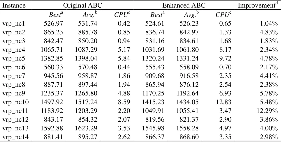
4.3 Original ABC vs. enhanced ABC
16
described operators as well as setting limit equal to 50n, and assessed by the set of 14 classical instances. Each test instance was run 20 times using each of the ABC heuristics. It was found that the speed of convergence of the two heuristics depends on n. Moreover, it was found that setting the termination condition (MaxIterations) to 2000n iterations is sufficient for the two heuristics to converge. The best results, the average results, the average CPU times obtained by the two versions for each test instance are also reported in Table 2, where the solution values recorded for both the best and average results are rounded to the nearest integer. According to this table, the enhanced version obtained better solutions than the original version in all test instances in terms of both the average and the best results in 20 runs. The mean percentage improvement of the average (best) results of all test instances is 4.16% (3.53%). The largest percentage improvement of the average (best) result is 12.29% (11.32%), indicating that the enhanced version can produce much better solutions than the basic version. From the table, we can observe that the enhanced ABC heuristic requires more computational effort than the original version. This is due to the modification of step 4d of the enhanced heuristic.
Table 2. Comparison of experimental results between the original and enhanced ABC heuristics
Instance Original ABC Enhanced ABC Improvementd
Besta Avg.b CPUc Besta Avg.b CPUc
vrp_nc1 526.97 531.74 0.42 524.61 526.23 0.65 1.04%
vrp_nc2 865.23 885.78 0.85 836.74 842.97 1.33 4.83%
vrp_nc3 842.47 850.20 0.94 831.16 834.61 1.68 1.83%
vrp_nc4 1065.71 1087.29 5.17 1031.69 1061.80 8.17 2.34%
vrp_nc5 1382.85 1398.04 5.84 1320.24 1331.24 9.72 4.78%
vrp_nc6 560.33 570.48 0.44 555.43 558.09 0.70 2.17%
vrp_nc7 945.56 958.87 1.86 909.68 916.58 2.35 4.41%
vrp_nc8 887.71 897.44 1.94 865.94 876.12 2.54 2.38%
vrp_nc9 1235.37 1265.80 4.88 1170.25 1192.64 6.93 5.78%
vrp_nc10 1497.92 1517.24 8.59 1415.23 1434.05 12.83 5.48%
vrp_nc11 1183.92 1203.29 2.20 1049.91 1055.41 3.47 12.29%
vrp_nc12 843.17 854.32 2.07 819.56 821.37 2.90 3.86%
vrp_nc13 1592.88 1623.29 3.53 1545.98 1558.28 4.97 4.00%
vrp_nc14 881.41 895.27 2.62 866.37 868.60 3.35 2.98%
a Best result obtained in 20 runs b Average result obtained in 20 runs
c Average CPU run time in minutes in 20 runs
d Percentage improvement of the average result obtained by the enhanced ABC over the original ABC
17
solution quality, we plot figures 11a and 11b. Figure 11a shows the plot of the best objective values found by the original ABC heuristic, the semi-enhanced ABC heuristic (where only step 4e is enhanced) and the enhanced ABC heuristic (both the steps 4d and 4e are enhanced) during one run on instance vrpnc1. It can be observed from the figure that the original and semi-enhanced ABC heuristics converge at the same rate, while the semi-enhanced version obtains a better solution. The enhanced variant converges at an earlier stage with a better solution than the other two variants.
Figure 11b shows the plot of the average objective values of the τ food sources obtained by the original, semi-enhanced and enhanced ABC heuristics at the different iterations during one run. The behaviors of the semi-enhanced and enhanced ABC heuristics are similar where the values are gradually lowered. On the opposite, the average objective values of the original ABC heuristic do not show this pattern and some fluctuations can be observed. Around 10,000 iterations, the original ABC heuristic has identified a minimum average objective value. However, the algorithm has not been able to improve this further but has given some fluctuation results. This is due to step 4e where
a food source xi will be replaced by a randomly generated solution if no improving neighbor
18 Figure 11. Converging processes of the basic ABC heuristic and its variants
In order to evaluate the effect of the modification made in step 4d on the average performance, we compared the average objective values of the semi-enhanced ABC heuristic with those of the enhanced one in figure 11b. It can be observed that the average objective values of the semi-enhanced variant are much worse than those of the semi-enhanced variant, which indicates that the modification made in step 4d significantly improves the quality of the search.
4.4 Computational results
Table 3 lists the characteristics of the 14 classical instances. For each test instance, the table indicates the number of customers (n), the vehicle capacity (Q), the service time (s) for each
19
Table 3. Enhanced ABC results for the classical instances
Instance n Q s L m Best known
b Obtained from Mester and Bräysy (2007)
c
Obtained from Rochat and Taillard (1995)
dAverage solution obtained by enhanced ABC in 20 runs e Best solution obtained by enhanced ABC in 20 runs f Deviation of ABC best from the best known solution
20
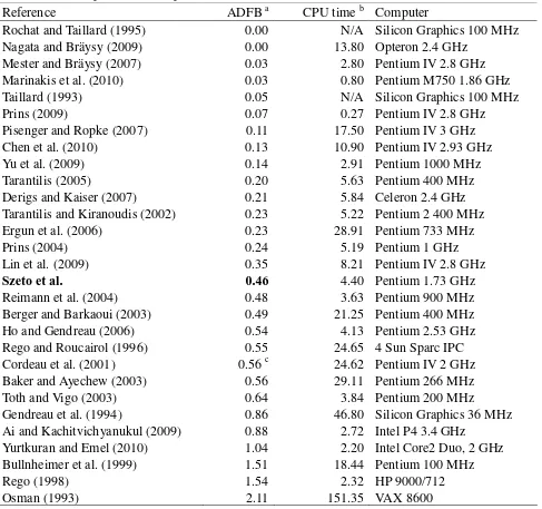
AGES algorithm (Mester and Bräysy, 2007) are also excellent.
Table 4. Comparison of computational results of different methods for the classical instances
Reference ADFB a CPU time b Computer
Rochat and Taillard (1995) 0.00 N/A Silicon Graphics 100 MHz Nagata and Bräysy (2009) 0.00 13.80 Opteron 2.4 GHz
Mester and Bräysy (2007) 0.03 2.80 Pentium IV 2.8 GHz Marinakis et al. (2010) 0.03 0.80 Pentium M750 1.86 GHz
Taillard (1993) 0.05 N/A Silicon Graphics 100 MHz
Prins (2009) 0.07 0.27 Pentium IV 2.8 GHz
Pisenger and Ropke (2007) 0.11 17.50 Pentium IV 3 GHz
Chen et al. (2010) 0.13 10.90 Pentium IV 2.93 GHz
Yu et al. (2009) 0.14 2.91 Pentium 1000 MHz
Tarantilis (2005) 0.20 5.63 Pentium 400 MHz
Derigs and Kaiser (2007) 0.21 5.84 Celeron 2.4 GHz Tarantilis and Kiranoudis (2002) 0.23 5.22 Pentium 2 400 MHz
Ergun et al. (2006) 0.23 28.91 Pentium 733 MHz
Prins (2004) 0.24 5.19 Pentium 1 GHz
Lin et al. (2009) 0.35 8.21 Pentium IV 2.8 GHz
Szeto et al. 0.46 4.40 Pentium 1.73 GHz
Reimann et al. (2004) 0.48 3.63 Pentium 900 MHz
Berger and Barkaoui (2003) 0.49 21.25 Pentium 400 MHz Ho and Gendreau (2006) 0.54 4.13 Pentium 2.53 GHz Rego and Roucairol (1996) 0.55 24.65 4 Sun Sparc IPC Cordeau et al. (2001) 0.56 c 24.62 Pentium IV 2 GHz Baker and Ayechew (2003) 0.56 29.11 Pentium 266 MHz
Toth and Vigo (2003) 0.64 3.84 Pentium 200 MHz
Gendreau et al. (1994) 0.86 46.80 Silicon Graphics 36 MHz Ai and Kachitvichyanukul (2009) 0.88 2.72 Intel P4 3.4 GHz
Yurtkuran and Emel (2010) 1.04 2.20 Intel Core2 Duo, 2 GHz Bullnheimer et al. (1999) 1.51 18.44 Pentium 100 MHz
Rego (1998) 1.54 2.32 HP 9000/712
Osman (1993) 2.11 151.35 VAX 8600
a Average deviation from best known results b Average computing time in minutes
c Computational results obtained from Cordeau et al. (2005)
21
computing environments. We believe that the reported CPU time for the enhanced ABC heuristic is reasonable and acceptable.
Table 5. Enhanced ABC results for the large-scale instances
Instance n Q s L m Best known
a Obtained from Nagata and Bräysy (2009) b Obtained from Prins (2004)
c Obtained from Prins (2009)
d Deviation from the best known solution
22
the classical instances, population-based heuristics combined with local search also generated the best results for the large-scale instances. From the table we notice that the memetic algorithm by Nagata and Bräysy (2009) and the AGES algorithm by Mester and Bräysy (2007) obtained much better solutions than the rest of the methods.
Table 6. Comparison of computational results of different methods for the
large-scale instances
Tarantilis (2005) 0.78 45.58 Pentium 400 MHz
Derigs and Kaiser (2007) 0.86 113.34 Celeron 2.4 GHz
Prins (2004) 1.09 66.90 Pentium 1 GHz
a Average deviation from best known results b Average computing time in minutes
c Computational results obtained from Cordeau et al. (2005)
5. Conclusions
23 Acknowledgements
The research was jointly supported by a grant (200902172003) from the Hui Oi Chow Trust Fund and two grants (201001159008 and 201011159026) from the University Research Committee of the University of Hong Kong. This support is gratefully acknowledged. Thanks are also due to the three anonymous referees for their valuable comments.
References
Ai TJ, Kachitvichyanukul V. Particle swarm optimization and two solution representations for solving the capacitated vehicle routing problem. Computers and Industrial Engineering 2009; 56; 380–387.
Baker BM, Ayechew MA. A genetic algorithm for the vehicle routing problem. Computers & Operations Research 2003; 30; 787-800.
Baldacci R, Toth P, Vigo D. Exact algorithms for routing problems under vehicle capacity constraints. Annals of Operations Research 2010; 175; 213-245.
Baykasoğlu A, Özbakir L, Tapkan P 2007. Artificial bee colony algorithm and its application to
generalized assignment problem. In: Chan FTS, Tiwari MK (Eds.). Swarm Intelligence: Focus on Ant and Particle Swarm Optimization. Vienna, Itech Education and Publishing; 2007. p. 113-144.
Berger J, Barkoui M. A new hybrid genetic algorithm for the capacitated vehicle routing problem. Journal of the Operational Research Society 2003; 54; 1254-1262.
Bullnheimer B, Hartl RF, Strauss C. An improved ant system algorithm for the vehicle routing problem. Annals of Operations Research 1999; 89; 319-328.
Chen P, Huang H-k, Dong X-Y. Iterated variable neighborhood descent algorithm for the capacitated vehicle routing problem. Expert Systems with Applications 2010; 37; 1620-1627. Christofides N, Eilon S. An algorithm for the vehicle dispatching problem. Operational Research
Quartely 1969; 20; 309-318.
Christofides N, Mingozzi A, Toth P 1979. The vehicle routing problem. In: Christofides N, Mingozzi A, Toth P, Sandi C (Eds.). Combinatorial Optimization. Chichester, Wiley; 1979. p. 315-338.
24
Cordeau J-F, Laporte G, Mercier A. A unified tabu search heuristic for vehicle routing problems with time windows. Journal of the Operational Research Society 2001; 52; 928-936.
Derigs U, Kaiser R. Applying the attribute based hill climber heuristic to the vehicle routing problem. European Journal of Operational Research 2007; 177; 719-732.
Ergun Ö, Orlin JB, Steele-Feldman A. Creating very large scale neighborhoods out of smaller ones by compounding moves. Journal of Heuristics 2006; 12; 115-140.
Gendreau M, Hertz A, Laporte G. A tabu search heuristic for the vehicle routing problem. Management Science 1994; 40; 1276-1290
Gendreau M, Laporte G, Potvin J-Y 2002. Metaheuristics for the capacitated VRP. In: Toth P, Vigo D (Eds.). The Vehicle Routing Problem. SIAM Society for Industrial and Applied Mathematics; 2002. p. 129-154.
Gendreau M, Potvin J-Y, Bräysy O, Hasle G, Løkketangen A 2008. Metaheuristics for the vehicle routing and its extensions: A categorized bibliography. In: Golden B, Raghavan S, Wasil E (Eds.). The vehicle routing problem: Latest advances and new challenges. Springer; 2008. p. 143-169.
Golden BL, Wasil EA, Kelly JP, Chao I-M 1998. Metaheuristics in vehicle routing. In: Crainic TG, Laporte G (Eds.). Fleet Management and Logistics. Kluwer; 1998. p. 33-56.
Ho SC, Gendreau M. Path relinking for the vehicle routing problem. Journal of Heuristics 2006; 12; 55-72.
Juan AA, Faulin J, Ruiz R, Barrios B, Caballé S. The SR-GCWS hybrid algorithm for solving the vehicle routing problem. Applied Soft Computing 2010; 10; 215-224.
Kang F, Li J, Xu Q. Structural inverse analysis by hybrid simplex artificial bee colony algorithms. Computers and Structures 2009; 87; 861-870.
Karaboga D. An idea based on honey bee swarm for numerical optimization. Technical Report TR06, Erciyes University; 2005.
Karaboga D, Basturk B. A powerful and efficient algorithm for numerical function optimization: artificial bee colony (ABC) algorithm. Journal of Global Optimization 2007; 39; 459-471. Karaboga D, Basturk B. On the performance of artificial bee colony (ABC) algorithm. Applied Soft
Computing 2008; 8; 687–697.
Karaboga D, Ozturk C. Neural networks training by artificial bee colony algorithm on pattern classification. Neural Network World 2009; 19; 279-292.
Karaboga N. A new design method based on artificial bee colony algorithm for digital IIR filters. Journal of the Franklin Institute 2009; 346; 328-348.
25
for very large scale vehicle routing problems. Computers & Operations Research 2007; 34; 2743-2757.
Li F, Golden B, Wasil E. Very large-scale vehicle routing: New test problems, algorithms, and results. Computers & Operations Research 2005; 32; 1165–1179.
Lin S-W, Lee Z-J, Ying K-C, Lee C-Y. Applying hybrid meta-heuristics for capacitated vehicle routing problem. Expert Systems with Applications 2009; 36; 1505-1512.
Marinakis Y, Marinaki M, Dounias G. Honey Bees Mating Optimization algorithm for large scale vehicle routing problems. Natural Computing 2010; 9; 5-27.
Mester D, Bräysy O. Active-guided evolution strategies for large-scale capacitated vehicle routing problems. Computers & Operations Research 2007; 34; 2964–2975.
Nagata Y, Bräysy O. Edge assembly-based memetic algorithm for the capacitated vehicle routing problem. Networks 2009; 54; 205–215.
Osman IH. Metastrategy simulated annealing and tabu search algorithms for the vehicle routing problem. Annals of Operations Research 1993; 41; 421-451.
Pisinger D, Ropke S. A general heuristic for vehicle routing problems. Computers & Operations Research 2007; 34; 2403-2435.
Prins C. A simple and effective evolutionary algorithm for the vehicle routing problem. Computers & Operations Research 2004; 31; 1985–2002.
Prins C 2009. A GRASP x Evolutionary local search hybrid for the vehicle routing problem. In: Pereira FB, Tavares J (Eds.). Bio-inspired Algorithms for the Vehicle Routing Problem. Springer-Verlag Berlin Heidelberg; 2009. p. 35-53.
Reimann M, Doerner K, Hartl RF. D-Ants: Savings Based Ants divide and conquer the vehicle routing problem. Computers & Operations Research 2004; 31; 563–591.
Rego C. A subpath ejection method for the vehicle routing problem. Management Science 1998; 44; 1447-1459.
Rego C, Roucairol C 1996. A parallel tabu search algorithm using ejection chains for the vehicle routing problem. In: Osman IH, Kelly P (Eds.). Meta-Heuristics: Theory and Applications, Boston, Kluwer; 1996. p. 661–675.
Rochat Y, Taillard É. Probabilistic diversification and intensification in local search for vehicle routing. Journal of Heuristics 1995; 1; 147-167.
Singh A. An artificial bee colony algorithm for the leaf-constrained minimum spanning tree problem. Applied Soft Computing 2009; 9; 625-631.
26
Tarantilis CD. Solving the vehicle routing problem with adaptive memory programming methodology. Computers & Operations Research 2005; 32; 2309–2327.
Tarantilis CD, Kiranoudis CT. BoneRoute: An adaptive memory-based method for effective fleet management. Annals of Operations Research 2002; 115; 227–241.
Toth P, Vigo D (Eds.). The Vehicle Routing Problem. SIAM Society for Industrial and Applied Mathematics, Philadelphia; 2002.
Toth P, Vigo D. The granular tabu search and its application to the vehicle-routing problem. Journal on Computing 2003; 15; 333–346.
Yu B, Yang Z-Z, Yao B. An improved ant colony optimization for vehicle routing problem. European Journal of Operational Research 2009; 196; 171–176.