Volume 26, Number 1, 2011, 25 – 46
GLANCING METEOR SHOWER OVER INDONESIA:
VOLATILITY SPILLOVERS FROM A MAJOR STOCK MARKET TO
INDONESIAN STOCK MARKET AND CURRENCY
Sekar Utami Setiastuti Durham University, United Kingdom
(s.u.setiastuti@durham.ac.uk)
ABSTRACT
During the deepest financial crisis in mid 2007-2009, increasing volatility of Indonesian stock market index were captured. Increasing volatility of the series is a common event since the volatility of financial market around the globe is increasing likewise. Yet, whether it is a sign of volatility spillover or comovement still emerges as a mystery.
This paper seeks to explain the causes of the increasing volatility in domestic currency and stock market. To investigates the hypothesis in tranquil and crisis periods, the observation period of January 2, 2003 to May 31, 2010 is splitted into two sub-periods with different levels of volatility. Using VAR-EGARCH on daily stock market index of Indonesia (IDX), S&P 500, and the bilateral exchange rate, we documented the existence of meteor shower and heatwaves in Indonesia stock market and exchange rate during crisis period. This finding implies that in crisis period, Indonesian stock market and exchange rate volatility were not only affected by market specific factors, but were also affected by volatility of the major stock market. We also captured asymmetric affects in the model which suggests that negative shock in the major stock market will increase the volatility of domestic stock market more than positive shock will.
Keywords: volatility spillovers, comovement, contagion, VAR-EGARCH
INTRODUCTION
Over the last two decades, we have seen several financial crises which originated in several markets and shortly after that spread across to other markets oceans away. Crises unravelled in the past show a highly integrated and globalised world and that disruptive events occured in one part of the world can have massive impact on a market on the other side of the globe. In the last two decades, financial markets were hit by a series of crises such as the European Exchange Rate Mechanism
(ERM) crisis, the 1994 Mexico’s peso
collapse, the 1997 East Asian crisis in 1992,
the Russian collapse in 1998, the Brazilian devaluation in 1999, the Information Technology (IT) stocks crisis in 2000, and the subprime mortgage crisis in the United States in 2008. A noteworthy feature during those crises is that markets tend to move more closely together as compared to tranquil times (Phylaktis and Xua, 2006). Such strong comovement is frequently referred to as
“contagion”. Evaluating whether contagion
Calvo and Mendoza (2000) indicated that crises in the 1990s were characterized by the following phenomena:
1. The crises were preceded by increasing ratios of public and private short-term liabilities relative to foreign reserves and by increased banking fragility—and not being preceded by expansionary policies (traditional culprits of currency crises). The crises were also preceded by the surge of portfolio capital inflows. Substantial reversals in capital flows preceed the crises.
2. Regardless of whether the currency remained stable or suffered a devaluation, a sudden stop of capital inflows will cause a sharp economic downturn and a boom in unemployment.
3. Crises started as country-specific episodes then quickly spread across financial markets within the same region and across the world. This form of contagion is believed to transmit capital markets vola-tility across countries which are unrelated by fundamentals.
Cross-border capital flows have been surging very rapidly, resulting in diversifi-cation of investments, financial market development in emerging economies, and a reduction in the cost of capital. The speed and magnitude of stock market development in developing countries have been remarkable and have resulted to fundamental shifts both in the financial structures of less developed countries and in the capital flows from developed nations (Cheung, et al., 2009).
A key indicator of stock market develop-ment, the capitalization ratio1 rose at a prodigious level in leading developing econo-mies during the 1980s and the 1990s, climbing from 10% to over 84% of GDP (Yartey, 2008). In Indonesia, the capitalization ratio has
1 Market capitalization as a proportion of GDP
reached 42% at the end of 20092 and the sign of linkage is getting more and more clear. In
January 20007, for example, foreign investors’
involvement was slightly over 20% of daily market total trading. In June 2010, the figure increased significantly to over 30%3. During the 2007-2009 global financial crisis, higher volatility of domestic currency and stock market indices were captured. But, whether this is a sign of volatility spillover or simply comovement between the domestic currency, domestic stock market, and the major foreign stock markets still has to be investigated. This paper tests the meteor shower hypothesis4, in the case of Indonesia during tranquil and crisis periods. Using the VAR-EGARCH model as in Koutmos (1996), we will be able to see the spillover, the magnitude, the direction, and the persistence of volatility.
EFFECT AND TRANSMISSION TO
EMERGING MARKETS
Contagion effects involved in financial and currency crises have been closely examined, especially in the aftermath of the 1997 Asian crisis (Masson, 1998; Corsetti, Pesenti and Roubini, 1999; Kaminsky and Reinhart, 1998a and 1998b). The contagion mechanism could be explained as the natural consequence of the real and financial interrelations between these economies. The mechanism also can be explained as a result of the actions of institutional investors which
have long positions in emerging markets’
financial instruments (Kaminsky and Schmukler, 1999). There are some channels of contagion that can be used to explain the transmission of a crisis in advanced financial
2 National Bureau of Statistics reported the nominal GDP
for 2009 at Rp 5,613 trillion and Indonesian Stock Exchange reported the 2009 market capitalization at Rp 2363 trillion
3 Source: Indonesia Stock Exchange Monthly Statistics
(January 2007 and Jnue 2010)
4
In Engle, et al. (1992), meteor shower is used as an analogy of volatility spillover effect between markets whereas heatwaves is used as analogy of volatility
markets spreading out to emerging currency markets.
A crisis might come from a drying-up of
investors’ liquidity (Cheung, et al., 2009). After a substantial price fall in a major market, investors have to suffer from a reduction of wealth and tend to withdraw their funds or raise cash by selling assets in other markets. The need for asset liquidation also may take place when a shock in one economy
diminishes the value of leveraged investors’
collateral, leading them to sell part of their holdings in unaffected economies to meet margin calls (Cheung, et al., 2009). For example, hedge funds may be highly leve-raged. Losses in one market worsen the value of their capital, leading to shrinkage of their portfolio size and consequently, liquidation of their holdings in other markets.
As all investors do the same thing at the same time, the crisis will spread over other regions. Convergence trading (Kyle and
Xiong, 2001), banks’ liabilities overlay across
countries, and marked-to-market valuations5 (Adrian and Shin, 2008) inflict liquidity tightening and provoke capital repatriation from emerging markets as well as a decline in bank loans. The financial linkages through which contagion can be transmitted can be more complicated in the presence of a chain of interconnected lenders (Cheung, et al., 2009).
A crisis also works as a “wake-up call” for investors6. This is related with the concept of portfolio rebalancing (Kaminsky and Reinhart, 1998). They will likely reassess their judgments and preferences after crises burst, especially on assets issued by countries of the same region, when they suddenly see other
5
When balance sheets are marked to market, asset-price changes will be reflected immediately on balance sheets and will trigger response from financial market participants
6 Hypothesis refers to the case where a crisis elsewhere
provides new information about the seriousness of problems in the home economy. This could sometimes be explained by similarities in the fundamentals and economic structure between economies.
financial assets appearing to be riskier, which
is said to trigger “flight to quality” (Caballero
and Krishnamurthy, 2005 and 2007). A crisis then might escalate risk aversion, which is confirmed by Kumar and Persaud (2002) and Coudert and Gex (2008). Investors with decreasing risk appetite may reexamine their
portfolio’s riskiness and choose to move their
portfolios toward less risky assets as their wealth declines (Cheung, et al., 2009). Furthermore, the high and extensive uncertainty during a crisis provokes herd behavior7 (Bickchandani and Sharma, 2000).
During turbulent times, financial markets tend to be more volatile. Bekaert and Harvey (1995) denote four sources of volatility differences: asset concentration, stock market development/economic integration, micro-structure effects8, and finally macroeconomic influences and political risk. However, whether a shock is transmitted, and whether it has a large impact on another country will depend very much on how vulnerable the real sector and financial system are. An economy is more vulnerable if it has weak macroeconomic fundamentals or financial system. The degree of vulnerability also increases with the number and size of linkages with the real economy and financial system of other economies (Bekaert and Harvey, 1995).
BACKGROUND THEORY
It is fascinating to see from the previous financial crises, how an initial market specific shock was rapidly transmitted to markets of very different sizes and structures around the globe. In currency crises, it is common to find crises triggered by severe attacks on other currencies, despite the weak linkages of trade
7 Different mechanisms help explain herding behaviour,
with some studies emphasizing asymmetric information. Information is costly to obtain, so less informed
investors may choose to follow the “leader”, and thus
will cause markets to move together
8 For example, the heterogeneity of traders’ information
and capital flow linkages among the eco-nomies concerned. The timing and virulence of the current crisis do not seem to be sufficiently explained by the fundamental problems facing many of the countries and markets concerned (Cheung, et al., 2009). This raises important questions about the nature of spillovers and contagion.
Bekaert and Harvey (1995) insinuate four distinguishing features of emerging market returns: higher average returns, low correla-tions with developed markets, predictability of returns is higher, and volatility is formidable. In developing and segmented capital markets, risk premiums may be directly related to the volatility of equity returns in the particular market.
Volatility is an important input for desicion making for asset allocation. In segmented capital markets, country volatility is a critical input in the cost of capital calculation and is more likely influenced by local factors (Bekaert and Harvey, 1995). Absence of volatility spillover implies that the major sources of disturbances are changes in asset or market-specific fundamentals, and large shocks increase the volatility only in the specific asset or market. On the other hand, the existence of volatility spillovers implies that one large shock increases the volatilities not only in its own asset or market but also in other assets or markets as well (Hong, 2001).
The volatility of foreign exchange rate markets plays a very important role in explaining equity return volatility (Bekaert and Harvey, 1995). Volatility in the foreign exchange rate is the one of the other major sources of macroeconomic uncertainty that affects the firms (Vardar, et al., 2008). A change in the exchange rates would affect a
firm’s foreign operation and overall profits, in
turn, affect its stock prices (Vardar et. al, 2008). Theoretical work such as Solnik (1974) and Adler and Dumas (1983) show that currency risk should be a priced factor in explaining equity returns. In other words,
developments in the currency market should affect the discount rate of firms. Dumas and Solnik (1995) use conditional asset pricing models to show that currency risk is important in explaining the variation in the mean of stock returns. Francis, et al. (2004) argue that exchange rates should affect the competi-tiveness of firms and thus their market values.
Many studies of the relationships between currency and equity treat exchange rate as exogenous. This fact can be due to traditional theoretical models of the determination of exchange rates having not calibrated the role for equity markets. Notwithstanding, tradi-tional (macroeconomic) models of exchange rates have been a failure in explaining exchange rate movements (Frankel and Rose, 1995). Flood and Rose (1995) concluded that the most critical determinants of exchange rate variability are not macroeconomic. Hau and Rey (2002) develop theoretical models in which exchange rates, stock prices and capital flows are jointly determined under incomplete foreign exchange risk trading. Both papers above show that exchange rates are impacted by equity returns. Specifically, Zapatero (1995) shows that exchange rate changes depend on the volatility of the domestic stock market and the covariance between the domestic and foreign stock markets. Currency volatility in his model is a function of the volatilities of both equity markets. In accor-dance with previously mentioned researches, we will employ bilateral exchange rate of US dollar and domestic currency (rupiah) to examine the impact of global financial market to the domestic financial market.
LITERATURE REVIEW
Spillover Between Stock Market Across Countries
correlation increases substantially, it suggests that the transmission between the two markets is magnified after the shock and thus contagion happens (Phylaktis and Xua, 2006). Hu, et al. (1997) examine the spillover effects of volatility among US and Japan and four emerging markets in the South China Growth Triangle (Hong Kong, Taiwan, Shanghai and Shenzhen) using the causality-in-variance test. Hilliard (1979) studied the contemporaneous and lagged correlation in daily closing price changes across 10 major stock markets. Jaffe and Westerfield (1985) examined daily closing prices in the Australian, Canadian, Japanese, UK, and U.S. stock markets. Eun and Shim (1989) studied daily stock returns across nine national stock markets. Barclay, Litzenberger, and Warner (1990) examined daily price volatility and volume for common stocks dually listed on the New York and Tokyo stock exchanges. They all found positive correlations in returns across individual stock exchanges.
The later studies suggest that focusing on correlations can be misleading. Forbes and Rigobon (2001) showed that using only unadjusted correlation coefficients is an inappropriate approach. The estimated corre-lation coefficient is an increasing function of the variance of the asset return, so that when coefficients between a calm period and a crisis period are compared, the coefficient in the crisis period is biased upwards as volatility rises substantially. In their research, In their research, Forbes and Rigobon (2001) showed that there is no contagion, only interdepen-dence between markets.
The later majority of studies examine the existence of volatility spillovers through autoregressive conditional heteroscedasticity (ARCH) family models. Most of these studies have found significant spillover effect across markets (Apergis and Rezitis, 2001). Koutmos and Booth (1995) found volatility spillovers from major stock markets, i.e. New York, London and Tokyo. Engle et al. (1992) and
Hogan and Melvin (1994) find the presence of meteor showers in international financial markets and indicate the presence of market inefficiency based on their failure to process all the available information efficiently.
In more recent work, the focus on volatility spillover has shifted towards detailed studies of the trading behaviour of foreign investors in an effort to detect herding beha-viour and other behabeha-vioural biases. Cho, Kho and Stulz (1999) find evidence of positive feedback trading and herding by foreign inves-tors before the Asian crisis, but not during the crisis period. They find no evidence that trades by foreign investors had a destabilizing effect on Korea's stock market, and found the market to adjust quickly and efficiently to large sales by foreign investors. Other studies that have examined the spillovers between international equity markets as most previous studies, have treated the currency market as exogenous or do not ascribe a specific role to the currency market in shaping these interdependencies (Francis, et al., 2004).
Spillovers Between Currencies
change in past Deutschemark volatility Granger-causes a change in current Japanese yen volatility, but a change in past Japanese yen volatility does not Granger-cause a change in current Deutschemark volatility. Apergis and Rezitis (2001) find no volatility spillover between these two exchange rates recorded on an hourly basis. While several other studies have examined spillovers in mean and volatility across currency markets (e.g. Baillie and Bollerslev, 1990; Engle, et al., 1990), they have not allowed for an influence from the equity markets.
De Santis and Gerard (1998) denote international investments are a combination of an investment in the foreign asset and an investment on the relative price of the two currencies involved (i.e. currency or exchange rate risk). Analysing whether volatility spillovers exist between the foreign exchange market and the equity market leads to a better understanding of the linkages between the two markets and the nature of risks that the participants in both markets have to cope with. In particular, increasingly high levels of cross-border equity flows lead to a higher demand for and supply of currencies (Tesar and Werner, 1995).
Spillover Between Stock Market and Exchange Rate
There are a growing number of researches that examine the dynamics of capital flows and equity returns. A change in the exchange rates
would affect a firm’s foreign operations and
overall profits, finally affecting its stock prices. Although the theoretical explanation is straightforward, earlier studies examining the relationship between stock markets and exchange rates showed mixed empirical findings. Mukherjee and Naka (1995), and Granger, Huang and Yang (2000) found a significant positive correlation while Kwon and Shin (1999) and Maysami and Koh (2000) reported a significant negative relationship. Tabak (2006), analyzing the dynamic relation
between stock prices and exchange rates in the Brazilian economy, showed that there is no long-term relationship between these variables.
Hamao, et al. (1990) found spillover effects from the U.S. and the U.K. stock markets to the Japanese market yet the effect shows an intriguing asymmetry: while the volatility spillover effect on the Japanese market is significant, the spillover effects on the other two markets are much weaker. Francis, et al. (2004) found significant, bi-directional mean and volatility spillovers between currency and equity markets and between US and foreign equity markets.
Francis, et al. (2004) indicate that signi-ficant mean and volatility spillovers are an important feature of the relationships between currency markets and domestic and foreign equity markets. Thus, excluding the exchange rate could lead to the conclusion that the foreign equity returns do not impact the mean of the domestic equity9. Similarly, studies of interdependence between currencies that exclude equity market returns may also inappropriately conclude that there are interdependencies between currencies, or may overstate their strength. This is because what would appear to be a spillover between currencies could be equity-to-currency spillovers, but the research design is incapable of capturing this (Francis, et al., 2004).
While vast research on volatility spillo-vers, market linkages, contagion between markets and between developed and developing markets has been produced, there is lack of attention to a segmented market like
Indonesia. The country’s stock market has
grown significantly in the past few years. Furthermore, it has been a decent performer among other markets in Asia10. Examining the
9 Because with the exclusion of the exchange rate the
spillover coefficient would represent the joint equity and currency impacts
10 From the early 2003 until early 2008, Jakarta
spillover from major markets can be fruitful for investment decisions and policy making. There is also lack of research focusing on the examination of the volatility spillover between major foreign stock markets to its domestic currency and stock market in two different time periods (e.g. tranquil/calm periods and crisis periods). Thus, this research aims to provide novel insight in the growing body of research in the volatility spillover field.
DATA AND STATISTICAL PROPERTIES Our study uses daily data of US and Indonesian stock market indices (S&P 500 Composite index and IDX Composite index), and rupiah-per-US dollar exchange rate. The daily return or change is computed using
100 Reuters DataStream. The sample period spans from January 2, 2003 to May 31, 2010. We break the full sample into two sub-periods, to examine the spillover effect in a tranquil period and a more volatile period.. The first period spans from January 2, 2003 to June 29, 2007 and the second period spans from July 2, 2007 to May 31, 2010. This period was chosen as in the early 2003, Indonesian market started to grow vastly and the proportion of foreign by the conviction of noisy series which mostly will be affected only by its specific factors. Nevertheless, using weekly or monthly data may block out interactions that last for a short period. There is significant time difference of 13 hours between US and Indonesia. Shocks
just 10 months. Nevertheless, the index sharply increased again in early 2009 and recorded a new level of 2,971.25 on April 2010.
that occur in the US market do not overlap
with Indonesia’s, thus shocks in the US market will affect Indonesia’s market on the following
day. For this reason, we lagged the US stock index data to be able to cope with this circumstance.
We use price index for indices data which means that the stock indices are not adjusted for dividends. Apergis and Rezitis (2001) denote that dividend adjustments do not affect the results, since the goal is to model second-order spillover effects. Specifically, dividends do not exhibit great variability, i.e. they are practically fixed. Consequently, adding them to the stock returns will affect only the mean of the returns and not their variability, which is the main objective of this study.
Table 1 provides some descriptive statistics of the daily returns for IDX, S&P 500, and the exchange rate for both sample periods. In period 1, the domestic market exhibits higher standard deviation (1.2%) compared to the US market (0.7%). This might be an early sign that volatility spillovers from developed markets to emerging markets do not occur. Nevertheless, in period 2, which is the crisis period, the standard deviation of the US market increases dramatically and reaches higher levels than for the Indonesian market. This result is intriguing as there might be a chance of meteor showers on the domestic market during the crisis period.
undergoes large fluctuations and in crisis periods, S&P 500 undergoes higher fluctuations than Indonesian market. All of the series have distributions with positive excess kurtosis and are seen to have heavy tails. The kurtosis exceeds 3, the distributions are not normal or said to be leptokurtic and this implies that the series contain extreme values. The Jarque-Bera test statistic also shows that normality is rejected for all return series in both periods.
Table 1. Descriptive Statistics
Period I IDX SP500 XR
Mean 0.00141 0.00048 -7.84E-06 Median 0.00086 0.00059 0 Maximum 0.05322 0.03481 0.03943 Minimum -0.07801 -0.03587 -0.02877 Std. Dev. 0.01205 0.00761 0.00493 Skewness -0.58095 -0.02476 0.62028 Kurtosis 7.23991 5.02399 12.18987
Jarque-Bera 925.272 196.239 4116.896 Probability 0 0 0
Sum 1.61420 0.54550 -0.00901 Sum Sq. Dev. 0.16674 0.06653 0.02787
Observations 1149 1149 1149
Period 2 IDX SP500 XR
Mean 0.00034 -0.00042 2.31E-05 Median 0.00021 0.00046 0 Maximum 0.07623 0.10957 0.07617 Minimum -0.10954 -0.09470 -0.06471 Std. Dev. 0.01895 0.01912 0.00621 Skewness -0.46955 -0.14679 1.36765 Kurtosis 7.99425 8.65135 50.64854
Jarque-Bera 817.774 1014.092 72132.390 Probability 0 0 0
Sum 0.25481 -0.32207 0.01759 Sum Sq. Dev. 0.27269 0.27736 0.02931
Observations 760 760 760
Table 2 shows the correlation coefficients of all series in both periods. From the table we can see that IDX is correlated to the S&P 500
with correlation coefficient of 0.277 in tranquil periods and the correlation increases in crisis periods (0.343). The same situation is reflected in the correlation between the S&P 500 index and the exchange rate and between the IDX index and the exchange rate. In crisis periods, both foreign and domestic stock markets exhibit higher negative correlation with the exchange rate.
We also analyse the movement of IDX and compare it to S&P 500 and the exchange rate from January 2, 2003 to May 31, 2010. Figure 1 presents all of the series with the exchange rate on the secondary axis. Compared to the S&P 500 index, the IDX index exhibits higher growth trends. From only 424 index points in January 2, 2003, the index boosted more than 500% to reach the level of 2,800 index point in early 2008. The Indonesian market was considered to be one of the top performers in the world, producing average growth of 50% annually. The ratio of capitalization (market capitalization to GDP) has also risen substantially. By the end of 2009, this ratio showed a figure of 36%. Both price index and market capitalization demonstrate the vast development of the Indonesian stock market. From late July 2007 to mid August, we spot a very interesting case where both S&P 500 and IDX broke a record and reached their peaks but immensely surging downward in less than three weeks. In the early 2008, when the S&P 500 index began to decrease, the IDX index seemed to be heavily affected. This is indicative of a selling spree in the US, which might have been caused by a decrease of
investors’ confidence or highly speculative
repatria-tion of capital, and worsening of confidence over the future of the economy.
In figure 2, we plot the return of the IDX index, the S&P 500 index, and the exchange rate for both periods. The figure provides information about the volatility of all series which can be seen after the crisis broke out, since returns of all series became more volatile. We spot a very high volatility of the exchange rate from the late-2008 to mid-2009 which indicates that there were large fluctuations of supply and demand for foreign currency (US dollar) in Indonesia. This might be due to the global financial crisis where capital mobility increases to meet the
investors’ return and risk objectives. De Santis and Gerard (1998) evidence that international investments involves buying assets in the foreign market, which makes investor exposed to market or country risk, and the investment of the relative price of the two currencies involved, which makes investors exposed to exchange rate risk. The flux of real economy and financial markets (i.e. stock market and bond market) thus profoundly affects the exchange rate of the domestic currency.
THE VAR AND MULTIVARIATE VAR-GARCH MODEL
While most studies in this field employ autoregressive conditional heteroscedasticity (ARCH) family models, some papers uses other methods such as Markov Switching regimes, excess residuals in VAR and cross-correlation analysis, as mentioned before. Unlike the other methods, the autoregressive conditional heteroskedastic (ARCH) model diagnoses the temporal dependence in the second moment of stock returns. This model was introduced by Engle (1982) and then later generalized by Bollerslev (1986). By analyzing the descriptive validity of these models, French, Schwert, and Stambaugh (1987) find that the generalized autoregressive conditional heteroskedasticity-in-mean (GARCH-M) model is a more attractive representation of daily stock-return behavior in the United States. The model successfully captured the effects of time-varying volatility on stocks’ expected returns. In this paper, a trivariate EGARCH(1,1) model is used to estimate the mean and volatility spillovers between the US and Indonesian stock markets and the bilateral exchange rate between the two countries.
Table 2. Correlation coefficients between daily market return in local currency and Rp/USD exchange rate and its p-value
Correlation Period 1 Correlation Period 2
Probability DLIDX DLSP500 DLXR Probability DLIDX DLSP500 DLXR
DLIDX 1 DLIDX 1
(---) (---)
DLSP500 0.276975* 1 DLSP500 0.343107* 1
(0.0000) (---) (0.0000) (---)
8000 8500 9000 9500 10000 10500 11000
0 500 1000 1500 2000
sp500 idx xr
8000 9000 10000 11000 12000 13000 14000
0 500 1000 1500 2000 2500 3000
sp500 idx xr
-.08 -.04 .00 .04 .08
2003 2004 2005 2006 2007
DLIDX
-.04 -.02 .00 .02 .04
2003 2004 2005 2006 2007
DLSP500
-.04 -.02 .00 .02 .04
2003 2004 2005 2006 2007
DLXR
Figure 2. Plot of volatility of IDXindex, S&P 500index, and Rp/USD exchange rate for period 1 and period 2
We use EGARCH(1,1) as an alternative of GARCH(1,1) model since it tends to perform better than traditional GARCH model (Pagan and Schwert, 1990). The model has several advantages over the pure GARCH specifi-cation. Traditional GARCH models ignores information on the direction of returns—only
the magnitude matters (Engle, 2001). It assumes that positive and negative error terms have a symmetric effect on the volatility11. In fact, the direction does affect volatility (Engle, 2001). Most of the time, volatility increases
11 This means good and bad news have the same effect on
more after bad news than after good news12. EGARCH also allows the parameters of ARCH and GARCH to be negative (Nelson, 1991). Balaban (2006) compared GARCH with other two alternative, which are EGARCH and another GARCH extension, which is GJR GARCH, and found that EGARCH is the best performer. Nevertheless, GARCH performance is negligibly less than the EGARCH model (1% at most).
We also use VAR to examine the inter-relationship among the series. If we want to study the comovement of volatility of stock markets, it is imperative to also analyze the market dynamics, transmission, and propagation mechanism which drives the series. We need to examine how shocks and volatility in one market are transmitted to other markets in a clearly recognizable fashion (Bala and Premaratne, 2008). To understand the mechanism, we have to look at the multilateral interaction between the series and to what extent it exists. We then have to focus on the structure of interdependence among stock markets and hence study all of the series as a single system (Bala and Premaratne, 2008). For identifying the channels of interactions, we employ a VAR model.
Multivariate GARCH model and VAR-EGARCH extensions
To capture the comovement and meteor shower effect between the S&P 500 index, the IDX index, and the exchange rate, we estimate a trivariate VAR-EGARCH model, as in Koutmos (1996). Modelling volatility of all of the series at the same time has several advantages over univariate approach or cross-correlation approach, in that this approach eliminates the two-step procedures and avoids problems associated with estimated regressors (Koutmos and Booth, 1995). This approach also improves the efficiency and the power of the tests for cross market comovement and
12 This concept is called leverage effect
spillovers and is consistent with the idea that spillover effects are manifestations of the impact of global shocks on any given market (Bala and Pramaratne, 2008).
The GARCH model was developed independently by Bollerslev (1986) and Taylor (1986) (Brooks, 2009). The GARCH model allows the conditional variance to be dependent upon previous own lags, so that the conditional variance equation in the simplest case is now: because it is a one-period ahead estimation of the variance calculated based on any past information thought relevant (Brooks, 2009). Brooks (2009) also explains that this model allows us to interpret the current fitted variance as a weighted function of a long-term average value, information about volatility in the previous period (1u2t1), and the fitted
If we rearrange the equation:
t
In this study, we use VAR-EGARCH(1,1)
where Ri,t is the return where i=1,2,3 (1 = S&P
500, 2 = IDX, and 3 = exchange rate). Ωt−1 is VAR system, in which the conditional mean in each series is a function of past own returns exponential function of past own, cross-series standarized innovations and past own conditional variance. The degree of volatility persistence is measured by i. If i1, the unconditional variance is finite. Thus if i=1,
then the unconditional variance does not exist.
ARCH effect is captured in equation (17), which is an asymmetric function of past standardized innovations and measures the magnitude effect and sign effect. The term
When the magnitude effect is greater than the expected value E(|vj,t1| ), the impact of past
standardized innovations on 2i,t(conditional
mean) will be greatly positive, if ai,j is
positive. If j is negative, a decline in series j
will be followed by larger volatility the other series (Koutmos, 1996). Hence, this parameter measures the asymmetric volatility trans-mission mechanism. If j0, a positive
shock will have the same effect as a negative shock of the same magnitude and if j1,
then a negative shock in a series will increase volatility of the other series while a positive shock will reduce the volatility.
The latter equation shows the conditional covariance specification, that captures the contemporaneous relationship among the returns of the three series. The specification implies that the covariance is proportional to the product of the standard deviations. The coefficient i,jis the cross-series correlation
coefficient of the standardized residuals bet-ween two markets (In et al., 2001). If this coefficient is significant, time-varying vola-tilities across series are correlated over time. This assumption simplifies the estimation of the model (Bollerslev et al., 1992). The log likelihood function for the multivariate EGARCH model is shown below:
vector of innovations at time t, St is the 3×3 time-varying conditional variance-covariance matrix with diagonal elements given in equation (16) for i,j=1,2,3 and cross-diagonal elements given in equation (18) for i,j=1,2,3 and i ≠ j. The log likelihood function is nonlinear in θ hence numerical maximization techniques have to be used (In et. al, 2001). In this paper, all multivariate EGARCH models and the diagnostic tests were conducted using winRATS 7.3 software.
Empirical Findings
Before we estimated VAR-EGARCH, we have to check whether the data are stationary and estimated the optimum lag to be used for VAR in the mean equation. Table 3 presents
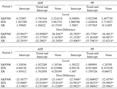
the test statistic of the ADF and Philips-Perron test. The tests indicate that all series are not stationary in level. Series in first difference are all stationary and thus we use the first differenced series in the rest of the estimation.
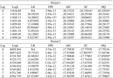
Table 4 shows the lag length criteria for the VAR system (both period 1 and period 2), from lag zero to lag eight. Final Prediction Error (FPE) and AIC (in period 1) and HQ (in period 2) chose lag 2 as the optimum lag to be used in VAR, but other criteria chose different optimum lag for both period. For example, SC and HQ chose lag 0 for period 1 and FPE and AIC chose lag 4 for period 2. To be consistent, we are going to use AIC as the criterion to decide the optimum lag.
Table 3. ADF and Philips-Perron test statistics in level and first difference
Period 1
ADF PP
Intercept Trend and
Intercept None Intercept
Trend and
Intercept None Level
S&P500 -0.32987 -2.795344 2.324118 -0.50894 -2.922308 2.487729 IDX 1.267289 -1.181839 3.961751 1.060786 -1.424816 3.713657 XR -1.59685 -1.56822 -0.13539 -1.5867 -1.557565 -0.13495
First Difference
S&P500 -25.9047* -25.89885* -36.2647* -36.7855* -3G.7794* -36.4013* IDX -13.2759* -13.37702* -5.16785* -31.3328* -31.36168* -30.9873* XR -25.2919* -25.2882* -25.3028* -33.8065* -33.79831* -33.8214*
Period 2
ADF PP
Intercept Trend and
Intercept None Intercept
Trend and
Intercept None Level
S&P500 -1.55036 -1.022289 -1.30746 -1.50222 -1.099991 -1.20705 IDX -0.88126 -0.915615 0.325986 -0.89138 -0.921869 0.347438 XR -1.85412 -1.762858 -0.20349 -1.487 -1.330726 -0.06072
First Difference
We then conducted lag exclusion test to get the optimum lag. For period 2, the test indicates lag 2 is better than lag 4. Hence, we continue the estimation with lag 2 in both period. Table 5 shows the stability of the VAR system for both periods. The table indicates that no root lies outside the unit circle for VAR system with lag 2. This implies that we are able to use VAR(2) system for the mean equation in the VAR-EGARCH system.
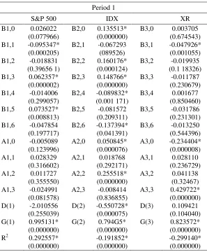
The maximum likelihood estimates of the full VAR(2)-EGARCH model are reported in table 6. B coefficients are the coefficients in the mean equation in period 2. With significant B coefficients in the mean equation for S&P 500 and IDX, this indicate that
domestic market returns are influenced by the world factor of US market and the exchange rate of rupiah to US dollar. The US returns will improve market sentiments in Indonesia leading to upward adjustments of earnings forecasts for the markets since returns in Indonesia increase when the US return increases. The significance of the return spillovers from the US can be attributed to the time difference of opening and closing hours between the markets in South East Asia and US13.
13 This is expected to influence the South East Asian
markets when they open 3-4 hours after the US market close (Samiri and Isa, 2009).
Table 4. Lag length criteria for VAR Period 1
Lag LogL LR FPE AIC SC HQ
0 11816.60 NA 2.96e-13 -20.33322 -20.32016* -20.32829* 1 11831.93 30.55510 2.93e-13 -20.34411 -20.29188 -20.32441 2 11849.13 34.20052 2.89e-13* -20.35823* -20Z6682 -20.32375 3 11853.40 8.457050 2.92e-13 -20.35008 -20.21950 -20.30082 4 11859.69 12.43800 2.93e-13 -20.34542 -20.17566 -20.28137 5 11874.65 29.50446* 2.90e-13 -20.35567 -20.14674 -20.27685 6 11881.18 12.85224 2.91e-13 -20.35143 -20.10332 -20.25782 7 11889.40 16.12865 2.92e-13 -20.35008 -20.06280 -20.24170 8 11894.26 9.521307 2.94e-13 -20.34297 -20.01651 -20.21980
Period 2
Lag LogL LR FPE AIC SC HQ
0 6659.564 NA 3.74e-12 -17.79830 -17.77978 -17.79116 1 6697.625 75.71523 3.46e- 12 -17.87600 -17.80193* -17.84746 2 6718.765 41.88263 3.35e-12 -17.90846 -17.77883 -17.85850* 3 6725.172 12.64256 3.37e-12 -17.90153 -17.71634 -17.83016 4 6739.690 28.53316 3.32e-12* -17.91628* -17.67554 -17.82351 5 6746.818 13.95079 3.34e-12 -17.91128 -17.61498 -17.79709 6 6749.082 4.412350 3.40e-12 -17.89327 -17.54141 -17.75767 7 6751.760 5.198067 3.46e- 12 -17.87636 -17.46895 -17.71936 8 6764.770 25.15106* 3.42e-12 -17.88709 -17.42411 -17.70867
* indicates lag order selected by the criterion
Table 5. VAR(2) stability condition
Period 1
Root Modulus
-0.019944 - 0.310290i 0.31093 -0.019944 + 0.310290i 0.31093 -0.024409 - 0.278817i 0.279884 -0.024409 + 0.278817i 0.279884 0.034672 - 0.187082i 0.190267 0.034672 + 0.187082i 0.190267 No root lies outside the unit circle.
VAR satisfies the stability condition.
Period 2
Root Modulus
-0.136777- 0.4045751 0.42707 -0.136777 + 0.4045751 0.42707
0.362125 0.362125
-0.097203 – 0.0755461 0.123109 -0.097203 + 0.0755461 0.123109
-0.04483 0.044831
No root lies outside the unit circle. VAR satisfies the stability condition.
Table 6. Maximum likelihood estimation of the VAR(2)-EGARCH Period 1
S&P 500 IDX XR
B1,0 0.026022 B2,0 0.135513* B3,0 0.003705
(0.077966) (0.000000) (0.674543)
B1,1 -0.095347* B2,1 -0.067293 B3,1 -0.047926*
(0.000205) (089526) (0.001055)
B1,2 -0.018831 B2,2 0.160176* B3,2 -0.019935
(0.39656 1) (0.000124) (0.1 18326)
B1,3 0.062357* B2,3 0.148766* B3,3 -0.011787
(0.000002) (0.000000) (0.230679)
B1,4 -0.014006 B2,4 -0.089832* B3,4 0.001677
(0.299057) (0.001 171) (0.850460)
B1,5 0.073527* B2,5 -0.081572 B3,5 -0.031786
(0.008813) (0.209311) (0.231301)
B1,6 -0.047854 B2,6 -0.137394* B3,6 -0.013250
(0.197717) (0.041391) (0.544396)
A1,0 -0.005089 A2,0 0.050845* A3,0 -0.234404*
(0.123996) (0.000076) (0.000008)
A1,1 0.028329 A2,1 0.018768 A3,1 0.028110
(0.316602) (0.292171) (0.236729)
A1,2 0.011727 A2,2 0.255518* A3,2 0.041138
(0.355550) (0.000000) (0.32467)
A1,3 -0.024991 A2,3 -0.008414 A3,3 0.429722*
(0.081578) (0.836855) (0.000000)
D(1) -2.010556 D(2) -0.550728* D(3) 0.109421
(0.255039) (0.000075) (0.104040)
G(1) 0.995131* G(2) 0.794G5* G(3) 0.823572*
(0.000000) (0.000000) (0.000000)
R2 0.292557* -0.191852* -0.299140*
Period 2
S&P 500 IDX XR
B1,0 -0.036796 B2,0 0.059381 B3,0 -0.011472
(0.201761) (0.152557) (0.235232)
B1,1 -0.221656* B2,1 0.034600 B3,1 -0.003065
(0.000000) (0.231544) (0.719457)
B 1,2 -0.031992 B2,2 0.1 10892* B3,2 -0.017103
(0.294030) (0.000607) (0.0641 60)
B1,3 0. 114708* B2,3 0.039154 B3,3 -0.012766
(0.000000) (0.235741) (0.074025)
B1,4 -0.000043 B2,4 -0.054984* B3,4 0.003678
(0.998867) (0.038130) (0.549471)
B1,5 -0.369380* B2,5 -0. 178124* B3,5 0.009571
(0.000099) (0.040134) (0.749511)
B1,6 -0.013018 B2,6 -0.300087* B3,6 0.020948
(0.875945) (0.000004) (0.5 1 1547)
A1,0 0.020981* A2,0 0.118265* A3,0 -0.008766
(0.008946) (0.000000) (0.109254)
A1, 1 0.1 66683* A2,1 0.1 16707* A3,1 0.107413*
(0.000000) (0.000712) (0.000019)
A1,2 0.022128 A2,2 0.133666* A3,2 0.057321*
(0.155623) (0.000139) (0.000002)
A1,3 -0.027383* A2,3 -0.001535 A3,3 0.031859
(0.021524) (0.932589) (0.057080)
D(1) -0.365126* D(2) -1.573535* D(3) -1.017275
(0.022259) (0.000003) (0.179231 )
G(1) 0.973215* G(2) 0.887140* G(3) 0.987375*
(0.000000) (0.000000) (0.000000)
R2 0.368893* -0.341116* -0.468805*
(0.000000) (0.000000) (0.000000)
* Denotes significance at the 5% level
Turning to the variance equation (vola-tility interaction), it can be seen in table 6 that in period 1, there is no spillovers effect from the S&P 500 index to the IDX index and to the exchange rate14 . Moreover, we find evidence of heatwaves in the IDX index and the exchange rate which shows that the volatility of both series is affected by its historical values. In period 2, we find significant volatility spillover from S&P 500 to IDX and the exchange rate. In this period, we also find heatwaves in S&P 500 and the IDX index, but not the exchange rate. Samiri and Isa (2009)
14 Shown by A2,1 and A3,1 coefficients which are not
significant
point out that more intense volatility spillovers are expected during the post-2007 period mainly due to the higher degree and persistence of volatility in the US market. In table 5, the degrees of volatility persistence are shown by the G parameter. Yet, unlike Samiri and Isa (2009), we find that although the degree of volatility of S&P 500 index is higher in the period 2, but it undergoes slightly higher volatility persistence in period 1. On the other hand, the IDX index and the exchange rate experience higher volatility persistence in period 2.
which is shown by the significant D(2) parameters. This finding is consistent with the notion that the volatility transmission mechanism is greatly determined by size and sign of the innovations. Nevertheless, for S&P 500, we only find asymmetric transmission mechanism in period 2. This finding implies that only in crisis period, negative news (shock) in S&P 500 increased volatility in domestic market and the exchange rate more than positive news did.
Table 7 shows the correlation coefficients of the standardized residuals in both periods. We can gauge that the correlations of S&P 500, IDX index, and exchange rate are higher in the crisis period. In tranquil periods, the coefficient of correlation for S&P 500 and IDX index is 0.29 and then slightly increases to 0.36 in crisis periods. For the exchange rate, the correlation to S&P 500 in tranquil periods is -0.19 and then increases to -0.33 in crisis periods.
Table 7. Correlation matrix between stan-darized innovations
Period 1
S&P 500 IDX XR S&P 500 1.00000 0.29678 -0.19462
IDX 1.00000 -0.30023
XR 1.00000
Period 2
S&P 500 IDX XR S&P 500 1.00000 0.36652 -0.33796
IDX 1.00000 -0.46554
XR 1.00000
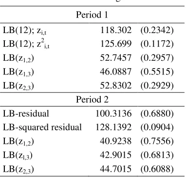
Model diagnostic tests in table 8 are based on the standardized residuals and show that the VAR(2)-EGARCH model satisfactorily explains the interactions of the three series in both periods. The Ljung-Box Q statistic shows no evidence of linear or non-linear dependence in the standardized residuals and standardized squared-residuals. The test for serial
corre-lation of the cross product of the standardized residuals shows the validity of constant correlation in each period, as in Koutmos (1996). The Ljung-Box statistic up to 12 lags, presented in table 8, shows no evidence of serial correlation so that the specification appears to be a reasonable parameterization of the variance-covariance structure of the three series.
Table 8. Model diagnostic
Period 1
LB(12); zi,t 118.302 (0.2342) LB(12); z2i,t 125.699 (0.1172) LB(z1,2) 52.7457 (0.2957) LB(z1,3) 46.0887 (0.5515) LB(z2,3) 52.8302 (0.2929)
Period 2
LB-residual 100.3136 (0.6880) LB-squared residual 128.1392 (0.0904) LB(z1,2) 40.9238 (0.7556) LB(zl,3) 42.9015 (0.6813) LB(z2,3) 44.7015 (0.6088)
CONCLUSIONS
Many studies have suggested that the development of financial integration has intensified contagion effects across markets. Capital flows from US to South East Asian markets has made the US the main source of international volatility to the region (Samiri and Isa, 2009). In Indonesia, not only market specific factors, but return and volatility in major stock markets, such as S&P 500 in the US, proved to affect the domestic stock market and exchange rates in the crisis period. We documented multidirectional lead/lag relation-ships between the S&P 500 and IDX indices in both (tranquil and crisis) periods. There are significant return and volatility spillover from S&P 500 to IDX index and exchange rate in crisis period. Volatility persistence is higher and the correlation of S&P 500 and IDX indices and exchange rate is also higher in the crisis period. The significant volatility spillover effects, coupled with negative significant asymmetric effect, implies that negative shock in the S&P 500 have a higher impact on the volatility of domestic stock market and the currency than positive shock. These analyses emphasize the existence of meteor showers and heatwaves in Indonesia over the last global financial crisis.
The empirical findings in this paper implies that the markets became more interdependent during the crisis period, and at the same time, more integrated in the sense that they each reacted not only to local news, but also to news originating in the major stock market. Developing financial markets such as Indonesia was proved to be affected by the financial crisis I in major market and the crisis has been undoubtely threatening the stability of domestic stock market. Government should ensure that they provide a sense of security and comfort to foreign investors, so they can withstand the rate of capital outflow from the domestic market and conceive a stable financial market, which at the end will make a positive contribution to economic growth.
REFERENCES
Adler, M. and Dumas, B., 1983, “International Portfolio Choice and Corporation Finance: A Synthesis”, Journal of Finance, 38(3), pp. 925-984.
Adrian, T. and Hyun, S.S, 2008, “Liquidity and Leverage”, Staff Reports 328, Federal Reserve Bank of New York.
Ahrens, R. and Reitz, S., 2003, “ Heteroge-neous Expectations In The Foreign Exchange Market Evidence from The Daily Dollar/DM Exchange Rate”, CFS Working Paper Series 2003/11.
Apergis, N. and Rezitis, A., 2001, “ Asym-metric Cross-Market Volatility Spillovers: Evidence From Daily Data on Equity and Foreign Exchange Markets”, Manchester School, University of Manchester, 69(0), pp: 81-96.
Baillie, R. T., and Bollerslev, T., 1989, “The Message in Daily Exchange Rates: A Conditional-Variance Tale”. Journal of Business & Economic Statistics, 7(3), pp: 60–68.
Barclay, M., Litzenberger, R., and Warner, J. , 1990, “Private Information, Trading Volume and Stock Return Variances”. Review of Financial Studies, 3, pp. 233– 253.
Bekaert, G. and Harvey, C.R., 1994, “ Time-Varying World Market Integration”, NBER Working Papers 4843.
Bekaert, G. and Harvey, C.R., 1995, “ Time-Varying World Market Integration”, Journal of Finance, 50(2), pp: 403-44. Bikhchandani, S. and Sharma, S., 2000, “Herd
Behavior in Financial Markets–A Review”, IMF Working Papers 00/48, International Monetary Fund.
Bollerslev, T., 1986, “Generalized Autore-gressive Conditional Heteroscedasticity”, Journal of Econometrics, 31, pp: 307‐27. Bollerslev, T., Chou, R.Y., and Kroner, K.F.,
Evidence”, Journal of Econometrics, 52, pp: 5-59.
Brooks, C., 2008, Introductory Econometric for Finance 2nd Edition. Cambridge: Cambridge University Press.
Caballero, R. J. and Krishnamurthy, A., 2007,
“Collective Risk Management in a Flight to Quality Episode”, NBER Working Papers 12896.
Caballero, R. J. and Krishnamurthy, A., 2005,
“Bubbles and Capital Flow Volatility: Causes and Risk Management”, NBER Working Papers 11618.
Calvo, G.A. and Mendoza, E.G., 2000,
“Capital-markets Crises and Economic Collapse in Emerging Markets: An Informational-Frictions Approach”, The American Economic Review, 90(2). Cheung, L., Chi-sang, T., and Szeto, J., 2009,
“Contagion of Financial Crises: A Literature Review of Theoretical and Empirical Frameworks”, Hongkong Monetary Authority Research Notes, 02/2009.
Cho, H., Kho, B.C and Stulz, R., 1999, “Do Foreign Investors Destabilize Stock Markets? The Korean Experience in 1997”. Journal of Financial Economics, 54(2).
Coudert, V. and Gex, M., 2008, “Contagion in The Credit Default Swap Market: The Case of The GM and Ford Crisis in 2005”, CEPII Working Papers, 2008(14). Corsetti, G., Pesenti, P., and Roubini, G.,
1998, “What Caused The Asian Currency And Financial Crises: Part I: A Macroeconomic Overview”, NBER Working Papers 6833.
De Santis, G., and Gerard, B., 1998, “How Big
is The Premium for Currency Risk”,
Journal of Financial Economics, 49(3), pp: 375-412.
Dumas, B. and Solnik, B., 1995, “The World Price Of Foreign Exchange Risk”. Journal of Finance ,50, pp. 445–479.
Enders, W., 1994, Applied Econometric Time Series, New York: John Wiley & Sons, Inc.
Engle, R.F., 1982, “Autoregressive Conditional Heteroscedasticity with Estimates of The Variance of United Kingdom Inflation”, Econometrica, 50(4), pp: 987-1007.
Engle, R.F., Ito, T. And Lin,W., 1992, “Where Does The Meteor Shower Come from? The Role of Stochastic Policy Coordination”, Journal of International Economics, 32(3-4), pp: 221-240. Eun, C.S. and Shim, S., 1989, “International
Transmission of Stock Market Movements”. Journal of Financial and Quantitative Analysis, 24, pp. 241–255. Flood, P.R. and Rose, A.K., 1995, “Fixing
Exchange Rates: A Virtual Quest for Fundamentals”, Journal of Monetary Economics, 36(1), pp: 3-37.
Forbes, K J. and Rigobon, R., 2002, “No Contagion, Only Interdependence: Measuring Stock Market Comovements”, Journal of Finance, 57, 2223-2261. Frankel, J.A., and Froot, K.A., 1986, The
Dollar as A Speculative Bubble: A Tale of Fundamentalists and Chartists. NBER Working Paper Series 1854.
Frankel, J.A and Rose, K.A., 1994, “A Survey of Empirical Research on Nominal Exchange Rate”, NBER Working Paper 4865.
French, K. R., Schwert, G. W., and Stambaugh, R. E., 1987, “Expected Stock Returns and Volatility”, Journal of Financial Economics, 19, pp: 3-29. Granger, C.W.J., Huang, B., and Yang, C.,
2000, “A Bivariate Causality Between Stock Prices and Exchange Rates: Evidence from Recent Asian Flu”, The Quarterly Review of Economics and Finance, 40, pp: 337-354.
Volatility Across International Stock Markets”, Review of Financial Studies, 3, pp: 281-307.
Hau, H. and Rey, H., 2002. “Exchange Rate, Equity Prices and Capital Flows”, NBER Working Papers 9398.
Hilliard, J.E., 1976, “The Relationship Between Equity Indices on World Exchanges”, Journal of Finance, 34(1), pp. 103-114.
Hogan, K. and Melvin, M.T., 1994, “Sources of Meteor Showers and Heat Waves in The Foreign Exchange Market”, Journal of International Economics, 37(3-4), pp: 239-247.
Hong, Y., 2001, “A Test for Volatility Spillover With Application to Exchange Rates”, Journal of Econometrics, 103(1-2), pp: 183-224.
Hu, J.W., Chen, M., and Fok, R.C.W., and Huang, B.N, 1997, “Causality in Volatility and Volatility Spillover Effects Between US, Japan and Four Equity Markets in The South China Growth Triangular”, Journal of International Financial Markets, 7, pp: 35l-367.
In, F., Kim, S., Yoon, J.H., and Viney, C., 2001, “Dynamic Interdependence and Volatility Transmission of Asian Stock Markets: Evidence from The Asian Crisis”, International Review of Financial Analysis, 10(2001), pp: 87-96.
Jaffe, J. and Westerfield R., 1985, “The Week-End Effect on Common Stock Return: The International Evidence”, The Wharton School Working Paper, 3(85).
Kaminsky, G. and Schmukler, S.L., 1999,
“What Triggers Market Jitters: A Chronicle of The Asian Crisis”, International Finance Discussion Papers 634, Board of Governors of the US Federal Reserve System.
Masson, P., 1998, “Contagion: Monsoonal Effects, Spillovers, and Jumps Between Multiple Equilibria”, IMF Working Paper, 98(142).
Koutmos, G., 1996, “Modeling The Dynamic Interdependence of Major European Stock Markets”. Journal of Business Finance and Accounting, 23, pp: 975-988.
Koutmos, G., & Booth, G. G., 1995,
“Asymmetric Volatility Transmission in International Stock Markets”, Journal of International Money and Finance, 14, pp: 747-762.
Kuhl, M., 2009, “Excess Comovements Between The Euro/US Dollar and British Pound/US Dollar Exchange Rates”, Center for European Governance and Economic Development Research Discussion Paper, 89(2009).
Kyle, A.S. and Xiong, W., 2001, “Contagion as A Wealth Effect”, Journal of Finance, 56:4.
Kwon, C.S. and T.S. Shin, T.S., 1999,
“Cointegration and Causality Between Macroeconomic Variables and Stock Market Returns”, Global Finance Journal, 10(1), pp: 71-81.
Maysami, R.C. and Koh, T.S., 2000, “A Vector Error Correction Model of The Singapore Stock Market”, International Review of Economics and Finance, 9, pp: 79-96.
Mukherjee, T.K. and Naka, A., 1995, “ Dyna-mic Relations Between MacroeconoDyna-mic Variables and The Japanese Stock Market: An Application of A Vector Error-Correction Model”. Journal of Financial Research, 18(2), pp. 223–237.
Phylaktis, K. and Xia, L., “Equity Market Comovement and Contagion: A Sectoral Perspective”. Available at http://www. ccfr.org.cn/cicf2006/cicf2006paper/20060 201013746.pdf.
Reinhart, C. and Kaminsky, G., 1998. “On Crises, Contagion, and Confusion”, MPRA Paper 13709, University Library of Munich, Germany.
Reinhart, C. and Kaminsky, G., 1998,
13877, University Library of Munich, Germany.
Samiri, A and Isa, Z., 2009, “The US Crisis and Volatility Spillover Across South East Asia Stock Markets”, International Research Journal of Finance and Economics, 34(2009).
Sola, M., Sapgnolo, F., and Spagnolo, N., 2001, “A Test for Volatility Spillover”. Available at http://www.carisma.brunel. ac.uk/papers/2.pdf.
Solnik, B.H., 1974, “An Equilibrium Model of The International Capital Market”, Journal of Economic Theory, 8, pp: 500-524.
Tabak, B.M., 2006. “The Dynamic Relation-ship Between Stock Prices and Exchange Rates: Evidence for Brazil”, Central Bank of Brazil Working Papers Series 124.
Tesar, L.L. and Werner, I.M., 1995, “Home Bias and High Turnover”, Journal of International Money and Finance, 14(4), pp: 467-492.
Vardar, G., Aksoy, G., and Can, E., 2008,
“Effects of Interest and Exchange Rate on Volatility and Return of Sector Price Indices at Istanbul Stock Exchange”, European Journal of Economics, Issue 11. Yartey, C.A., 2008, “The Determinants Of Stock Market Development in Emerging Economies: Is South Africa Different”, IMF Working Papers, 08(32).