Testing the convergence hypothesis for OECD countries: a reappraisal

(1)

Received October 30, 2016 Published as Economics Discussion Paper November 10, 2016

Testing the convergence hypothesis for OECD

countries: a reappraisal

Maria Dolores Gadea Rivas and Isabel Sanz Villarroya

Abstract

This paper reviews the results of a number of empirical studies of convergence among the OECD countries and discusses some limitations of these studies. Moreover, the paper tries to deal with these limitations by presenting a new and more appropriate methodology: quantile regressions. The results obtained with this specification support the view that, even among the OECD countries, there are different clusters. The parameter representing the convergence hypothesis, despite being negative in every case, is higher in value and more significant as we advance to higher quantiles. These outcomes reveal a faster convergence between the countries that belong to the upper quantiles. Moreover, 1960–1970 is highlighted as the period in which convergence was more intense.

JEL C32 O11

Keywords Convergence; quantile regression

Authors

Maria Dolores Gadea Rivas, Department of Applied Economics, University of Zaragoza, Zaragoza, Spain, lgadea@unizar.es

Isabel Sanz Villarroya, Department of Applied Economics, University of Zaragoza, Zaragoza,

Spain

Citation Maria Dolores Gadea Rivas and Isabel Sanz Villarroya (2017). Testing the convergence hypothesis for

(2)

1 Introduction

Since Barros (1991) pioneering proposals, the phenomenon of economic conver-gence between countries has been widely and empirically studied. These studies use the exogenous theory because it is the theory from which the concept of con-vergence arises. It is based on the Solow growth model, according to which, if different countries have the same preferences and technology, given the existence of decreasing marginal returns in the use of accumulating factors, especially capital, poor countries tend to grow faster than rich ones. Each country would attain its own steady state but, in the meantime, its differences in per capita income would tend to diminish.1 So, this theory predicts a process of catching-up (conditional conver-gence). Another possible solution can be observed when rich and poor countries reach the same steady state of income level, which forms the strict definition of convergence (absolute or unconditional).2

The vast majority of studies in this field focus on homogenous and developed samples made up, for example, of the European countries or the states of the USA, but above all, the OECD members are typically used as a case of study, especially after the Second World War. However, the results obtained are not conclusive and depend on the type of data and the econometric technique used.

Following Bernard and Durlauf (1995, 1996), we must underline that the ex-ogenous growth theory has serious inconveniences when tested empirically. The fundamental shortcoming is that the concept of convergence is not explicitly defined and tends to be confused with catching-up. For them, the strict definition of conver-gence means the equalization of income levels per capita at a given time while the reduction of distances in per capita income is related to the concept of conditional convergence, that is, catching-up.

A second shortcoming when testing this theory empirically derives from using cross-sectional data or, in the best of cases, panel data, as a pioneering work of Islam (1995) does. The problem in both scenarios is that the analysis offers results that do not allow us to distinguish between the short term and the long term. The results do not describe the process profile and do not permit a distinction between strict convergence and catching-up, as Bernard and Durlauf (1995), Zivot and Andrews (1992) and Greasley and Oxley (1998) among others, highlight.

Last but not least, there is the additional problem of defining the null hypothesis. In this type of analysis, the null hypothesis maintains that none of the countries considered converges, whereas the alternative hypothesis maintains that all countries

1 _{Neoclassical theory does not have universal acceptance. It is possible to find rich countries that grow}

faster than poor countries and vice versa. This has been denied by economists who have proposed an endogenous growth theory. Its leading representatives are Romer (1986, 1990) and Lucas (1988, 1990). This group of scholars argue, contrary to neoclassical reasoning, that the differences in GDP per capita can persist ad infinitum due to constant or increasing marginal returns.

2 _{A concept of convergence that derives from the exogenous theory assuming equality of conditioning}

(3)

converge without taking intermediate situations into consideration, something that Bernard and Durlauf (1995, 1996) also highlight.

To deal with these problems, more recent approximations consider time-series data – a type of data capable of representing the behavior of countries in the long term – and structure the analysis of convergence and catching-up within the theoretical framework of time series using either cointegration techniques3_or univariate analysis of GDP per capita series of the countries under consideration.4

As we noted earlier, the empirical studies using the OECD countries as a sample have reached different conclusions if the cross-sectional, panel or time-series approaches are used for periods of time that cover from the 1950s to the 1990s. For example, Baumol (1986), Barro (1991), Mankiw et al. (1992) and Sala-i-Martín (1996), using cross sectional data find convergence, something that is intensified when using panel data in the respective studies of Islam (1995) and De la Fuente (1997).

However, Bernard and Durlauf (1995, 1996) reject this hypothesis of conver-gence for the OECD using time-series data while Nahar and Inder (2002), with a different technique, find convergence for 19 out of 21 countries in the OECD sample considered.

With a different time series methodology, Bentzen (2005) find that the catching-up process that is observed for most OECD countries with respect to the USA presents stages of progress and retreat, specific for each country. Datta (2003) and Epstein et al. (2003) obtain the same results when considering a historical period that begins in 1870. Other more recent works in the field of time series, using other techniques, do not coincide completely with these previous authors. Rassekh et al. (2001), for example, find convergence only for the Golden Age.

Studies such as Mello and Perrelli (2003) and Ram (2008) apply the quantile regressions methodology with cross-sectional data and find evidence of convergence only for the upper tail of the OECD countries during 1960–1998.

Therefore, there is no consensus in the results and they depend on the methodol-ogy and the technique used. As a consequence, the following questions arise: what conclusion can we reach? which kind of data is most appropriate? Is it possible to find a better method to test the convergence hypothesis?

In order to answer these questions, this paper starts with a selective survey of the empirical literature on convergence for the OECD countries. We summarize the main results of this literature and examine their implications and shortcomings and present a new methodology that attempts to deal with some of the problems that previous research has been unable to resolve.

To this end, the convergence debate is re-examined using quantile regressions on 21 OECD countries over a panel of data which explores the cross-sectional and the time dimensions of the data. The challenge is to explain the observed patterns of cross-country income distribution dynamics that lead to the formation of clubs of

3 _{Bernard and Durlauf (1995).}

(4)

economies that follow different development paths and converge to distinct steady states.

The results obtained imply a faster convergence between the countries that belong to the upper quantiles and highlight 1960–1970 as the period in which convergence was more intense.

2 What other research says about convergence

2.1 The initial approaches

In recent convergence studies, the neoclassical theory has been widely accepted. This theory is represented in the Solow growth model, according to which, if different countries have the same preferences and technology, given the existence of decreasing marginal returns in the use of accumulating factors, especially capital, poor countries tend to grow faster than rich ones. They will, thus, have the chance to close the gap between them or even to reach the same level of GDP. In fact, this possibility does not derive directly from the neoclassical theory unless a number of assumptions concerning the accumulating factors are imposed. This represents a process of absolute convergence in which all countries under consideration will meet at the same point or steady state. This is known as unconditional convergence (unconditionalβ-convergence).5

The alternative, that of closing the gap, is associated with a concept of weaker convergence known as conditional convergence, arising from the implications of Solows model which predicts convergence after taking into account the factors which determine the steady state equilibrium (conditionalβ-convergence). These are the savings rate (physical capital is used as proxy) and the growth rate of the population. The full version of this model includes human capital as an additional variable of the steady state.6

In this context of conditional convergence, the differences in per capita income between rich and poor countries will tend to decrease, while each country will reach

5 _Parameter_β_{, which indicates the presence of unconditional convergence, is calculated using the} following estimation:(1/T)∗ln(Yi,to+T/Yi,t0) =a−[(1−e−βT)/T]∗ln(Yi,t0); whereY represents GDP per capita.

6 _{A different way to measure convergence is to use the typical deviation of GDP per capita over time,}

(5)

its point of equilibrium.7 Each country would attain its own steady state but in the meantime its differences in per capita income would tend to diminish.8

Since Barros pioneering proposals, the phenomenon of economic convergence between countries has been widely studied empirically9and the vast majority of studies in this field focus on developed countries, especially on OECD economies, EU countries and the states of the USA.

Earlier studies, including Baumol (1986), Barro (1991), Mankiw et al. (1992) and Sala-i-Martín (1996) offer strong evidence of convergence for the OECD countries, either conditional or unconditional. However, these studies analyze the cross-sectional correlation between initial per capita output levels and subsequent growth rates for a group of countries. A negative correlation is taken as evidence of convergence as it implies that, on average, countries with a low per capita initial income are growing faster than those with a high initial per capita income. So, in this type of analysis, the null hypothesis maintains that none of the countries considered converges, whereas the alternative hypothesis maintains that all countries converge without taking intermediate situations into consideration (Bernard and Durlauf 1995, 1996) which is a shortcoming of this approach.

Another weakness of cross-sectional tests is that the analysis offers results that do not allow us to distinguish between the short and the long term and they are limited when it comes to investigating the process of absolute or unconditional convergence or the tendency towards catching-up. Cross-sectional tests do not provide evidence of the existence of long-run income convergence but long-run convergence is the only way to differentiate between the attainment of income equality and catching-up. Another drawback of this type of data is that time is not taken into account, eliminating the information contained in the sample regarding the effects of changes in growth and showing only differences between countries.

The use of panel data to test the convergence hypothesis has some various advan-tages over cross-sectional data. First, they permit the introduction of dynamism into the models by introducing lags into the specification. Second, and more important, the use of panel data enables us to discern whether the estimated coefficients really reflect the impact of the exogenous variables or whether, on the contrary, they are due to the unobserved individual effects that are correlated with them. Additionally, the panel data estimations increase the accuracy of the estimator and allow us to increment the degree of freedom.10

7 _{As suggested by Barro and Sala-i-Martín, the estimate for parameter}_β _{indicating the presence} of convergence is calculated using this estimate(1/T)∗ln(Yi,to+T/Yi,t0) =a−[(1−e−βT)/T]∗ ln(Yi,t0)+other variables; whereY represents the variable GDP per head. See Barro, R.J. and X. Sala-i-Martín (1995: 223–251).

8 _{Neoclassical theory is not universally accepted; we can find rich countries that grow faster than poor}

countries and vice versa. This has been examined by economists who have proposed an endogenous growth theory. Its leading representatives are Romer (1986, 1990) and Lucas (1988, 1990). This group of scholars maintains, contrary to neo-classical reasoning, that the differences in GDP per capita can persist ad infinitum given that there may be constant or increasing marginal returns.

9 _{Barro (1991).}

(6)

Using this kind of data, Islam (1995) found higher rates of both conditional and unconditional convergence over the OECD sample in the period 1960–1985 than those obtained from single cross-country regressions. De la Fuente (1997) reaches the same conclusion.

However, panel data approximations do not resolve the issue of distinguishing clearly between the short and the long term, nor is it possible to describe the profile of the convergence process. With this kind of data it is not possible to detect which countries of the sample are converging and which are not.

2.2 The new and alternative approaches

To avoid the problems mentioned in the previous section, more recent approxima-tions take into account time-series data and structure the analysis of convergence and catching-up within the theoretical framework of time series using either cointe-gration techniques or univariate analysis of GDP per capita series of the countries under consideration. In the first of the two cases mentioned, Bernard y Durlauf (1995, 1996),11using cointegration techniques and data for 15 OECD countries over the period 1950–1987, rejected the convergence hypothesis. They consider that when the difference of income per capita between two countries is a stationary process with zero mean there will be a cointegration relation between them and the strict definition of convergence holds.12 If, on the contrary, they do not maintain a steady trend throughout the period, this indicates a weak version of convergence, i.e. catching up, and will be reflected in the persistence of different steady states over time. They, therefore interpret the convergence hypothesis as implying that output differences are transitory, that is, the process is mean zero stationary.

Another type of analysis with time series is that performed by Greasley and Oxley (1998) considering a pair-wise convergence for a similar set of data as that used by Bernard and Durlauf (1995). These authors, applying the proposals made by Perron (1989) and, especially, by Zivot and Andrews (1992), found some mild evidence of stochastic convergence between pairs of a set of countries formed by Australia, Canada and the USA.13 Following Greasley and Oxley (1998), if this

11_{Bernard and Durlauf (1995, 1996) distinguish between the two definitions in the following way:}

Output convergence: “two countriesiandjconverge if the logarithm of output per capita for both countries is the same at a given moment”.

limk→∞E(yi,t+k−yj,t+k/It) =0

Catching-up convergence: “two countriesiandjconverge between two moments of timetand t+T, if the differences in the logarithm of output per capita in t diminishes in value at momentt+T. IfYi,t>Yj,tthen:

E(yi,t+T−yj,t+k/It)<yi,t−yj,t

In both cases,Y is the logarithm of output per capita, and It is the information available at time t. The first definition implies the second and also that these definitions can be generalized for the multivariate case.

12_{Bernard and Durlauf (1995).}

13_{It is important to remember that, according to Perron (1989), we often admit the unit root hypothesis}

(7)

comparative series is not stationary, the strict definition of convergence will not hold, given that any shock will persist and prevent the process of convergence.14 Nevertheless if this relative series shows a segmented trend, we can deduce a process of catching-up but not of strict convergence. There would be no long-term convergence given that the structural breaks indicate that equal GDP levels, if they had existed at any time, could not be maintained. Even so, the observed breaks do not necessarily impede a reduction in the differences in per capita income. In fact, on the contrary, they may contribute to the existence of such a reduction.

In sum, most of the empirical studies that have used time-series data have failed to find convincing evidence of convergence for real per capita GDP between OECD countries. A notable exception is the study of Nahar and Inder (2002) who find convergence to the mean for at least 19 of the 21 OECD countries and that the vast majority of these countries are converging towards the USA. These authors work with two concepts of convergence, one based on whether a countrys output gap from the leader, the USA, is declining and the other looking at whether there is a decline in the difference between the per capita GDP of a country and the average per capita GDP of all the countries in the group. The first of these it defines the difference between the per capita GDP of a country and that of the USA as a function over time. As all the countries have a negative difference, for convergence to hold, the slope of this function is expected to be positive over time, indicating that the countrys is difference with the leader decreases over time. The authors find strong evidence of convergence for all countries except Switzerland and New Zealand. Nahar and Inder maintain that there must be a positive and significant trend in the output gap, and criticize the position of Bernard and Durlauf. A model with a positive linear trend and stationary error, like that proposed by Bernard and Durlauf, would actually be inconsistent with the definition of convergence because the long-term forecast of the output gap would not converge to zero.15 In the second analysis, when comparing the per capita GDP of each country with respect to the average of the sample, another function of differences is defined. In this case, it has positive and negative values as the countries perform above or below the average. This function is defined squarely so for convergence to hold, it should always be getting closer to cero. That is, if the economy tends to converge, the slope function of this squared funtion will be negative. The outcomes reflect convergence for all countries except Germany, Iceland and Norway. Based on this last study, Bentzen (2005) replicates the avobementioned Nahar and Inder (2002) analysis for a group of 20 OECD countries during the period 1950–2000 and confirms the idea that the

hypothesis in statistical tests like that of Dickey–Fuller (see e.g. Dickey and Fuller (1979, 1981)). Perron proposes a formal test of structural changes which consists of introducing a dummy variable into the augmented Dickey–Fuller equation that represents the moment in which we observe the structural change.

14_{It is important to stress that, when we perform a univariate analysis of an individual series, the}

(8)

majority of them were catching up with the USA. Moreover, using the QLR test, he detects some important breaks that modulate the catch-up process and show it loses speed after each of these breaks. Depending on the country, the breaks are situated at the end of the sixties, the beginning of the seventies, the mid-seventies or, even, the beginning of the eighties, indicating that country-specific causes are most likely driving these catching-up processes.

Epstein et al. (2003) reach a similar conclusion using a distribution dynamics approach for a sample of 17 OECD countries during the period 1870–1992 in order to better capture what happens in the transition to the steady state. This analysis uses a Kernel density estimator and is in line with Quah (1993, 1996, 1997) who argues that only by considering the issues of growth and distribution simultaneously can we understand their underlying dynamics. Epstein at al. (2003) improve in the previous literature by focusing on the movement of economies between different income levels, showing tendencies to cluster around a certain income level and to stratification, that is, where economies move into distinct income-level strata. The main objective of the paper is to detect whether relatively rich and poor countries remain relatively rich and poor over time. They conclude that, for the period as a whole, there is a convergence process simply because the countries that move to a lower income state outnumbered those that move to a higher income state. Nevertheless, looking at the change in distribution over tim,e they confirm that convergence is mainly a feature of the Golden Age (1950–1973) in this set of countries; afterwards, separation, polarization and divergence were the rule.

Another test that partially confirms the outcomes described above and attempts to deal with the problems associated with the two popular tests of convergence,

β-convergence and theσ-convergence, is that of Rassekh, Panik and Kolluri (2001). It is based on other methodologies such as the ARMA process estimation applied over two different measures of theσ convergence series.16 The first measure is calculated using the actual dispersion between the GDP levels of 24 OECD countries in the period 1950–1990. The secondσ measure is calculated using the adjusted residuals obtained after estimating a growth equation that accounts for the main factors such as investment, government consumption and exports as a share of GDP, that is, the Solow residual. The idea here is to capture how the unexplained component of growth is attributed specifically to the convergence process. The reason is that the faster growth of the lower-income countries in the sample may be due to greater investment or to some other growth-inducing policies rather than to real convergence forces. If this adjustedσmeasure does not decline over time, then any tendency of countries to converge must be attributable to the determinants of growth and this would reject the convergence hypothesis for the sample of countries even though statistical convergence might be found using the actual measure ofσ. This was, in fact, the case although both the indicators, -the actual and the adjusted

(9)

measures ofσ -, decline over time, the ARMA procedure rejects the convergence hypothesis for the entire period because both series are non-stationary. Nevertheless, when the sample was split into two periods determined by the recursive Chow test, from 1950 to 1977 and afterwards, modest support for the hypothesis was only found during the first, that is, during the Golden Age.

Datta (2003) adopts the Kalman filter procedure to capture the dynamic be-haviour and does not reach the same conclusion. The constant parameter coin-tegration model required to test whether the linear combination of two series is stationary is based on the assumption that the long-run relationship between them is time-invariant and linear. This assumption is very appropriate to test for steady state behaviour, as Bernard and Durlauf point out but, in fact, some countries may not have reached their steady state and may still be in transition. The process of convergence may also be nonlinear and may exhibit structural changes. In this paper, the author examines both of these possibilities using a pairwise series looking at series of the difference between the GDP of an OECD country and the leader, the USA, during the period 1950–1992. The methodology confirms that the growth path for the countries is dynamic with cyclical trends, which shows shows how the assumption of structural stability is not appropriate and means that the economies under consideration are far from their steady states even though a process of catch-up among the OECD countries existed during this period. These results help to explain why the time-series conclusions on convergence differ from the cross-sectional results, even for the same set of countries.

From the above discussion, it is clear that, for similar data sets, the results of different approaches are contradictory. The time-series approach resolves some of the shortcomings presented in the cross-sectional and panel approximations but leaves some crucial points unanswered. In particular, even if the relative time series show a segmented trend, we are not able to observe the existence of different steady states where a set of countries converges during a certain time. We can only see how a country converges or is catching up with the leader (or with an average income). This disadvantage is, in part, resolved using the Kernel density methodology, as Epstein et al. (2003) do, but even this method does not allow for the possibility of several steady states that define different clubs of countries. It only shows how the economies are moving towards distinct income-level strata.

(10)

Mello and Perrelli (2003) and Ram (2008,) using this methodology for a broad sample, find evidence of unconditional convergence for countries in the upper tail of the conditional growth distribution but not for those in the lower tail. They find evidence of convergence for the whole set of OECD countries only in the upper tail of the conditional growth distribution, and for different sub-samples of OECD countries. According to their estimates, the OECD converged at a faster pace in 1960–1998 than in 1960–1985. However, the problem with the approach developed is that the possibility of applying this methodology using panel data is not explored.

Quantile regression with panel data has the advantage that, if the sample is split into sub-periods of time, it is possible to analyse the transition dynamic of the convergence process and reach conclusions about the set of countries and about the period for which our hypothesis is maintained. For these reasons, this methodology resolves several deficiencies that the cross-sectional and time-series estimations present. Is it possible to reach the same conclusions for the OECD countries using quantile regressions with panel data? Is convergence a story that only involves a few countries? In which period is the convergence process stronger?

A more detailed description of this methodology and the results obtained appear in the following sections.

3 A quantile approach for convergence

3.1 The data

Our database includes a total of 21 OECD countries17for 10 periods of 5 years.18 Data of per capita income are in 1990 international Geary-Khamis dollars and are obtained from Penn World tables. We have considered the average growth rate of per capita income every 5 yearsyc,t and its initial value in each quinquenniumxc,t

wherecrepresents the country withc=1...21 andt=1...10 the periods.

3.2 The method

In order to examine the empirical performance of the convergence, both a standard and a quantile panel regression analysis have been carried out.19 For the standard panel regression analysis, the following model has been considered

yc,t =θi+xc′,tβ+uc,t, (1)

17_{These countries are Australia (AU), Austria (AT), Belgium (BE), Canada (CA), Denmark (DK),}

Finland (FI), France (FR), Germany (GE), Greece (GR), Ireland (IR), Italy (IT), Japan (JP), New Zealand (NZ), the Netherlands (NH), Norway (NO), Portugal (PO), Spain (SP), Sweden (SW), Switzerland (SZ), the United Kingdom (UK) and the United States (US).

18_{These periods are 1950–1955, 1955–1960, 1960–1965, 1965–1970, 1970–1975, 1975–1980, 1980–}

1985, 1985–1990, 1990–1995 and 1995–2000.

19_{Previously, a panel unit root analysis has been carried out. Both the test of Levin et al. (2002) and}

(11)

where (yc,t,xc,t)denote the values of the dependent ( the average growth rate of

per capita income every 5 years) and independent variables (the initial value of per capita income in each quinquennium), respectively, andican take valuecor

tdepending on whether fixed effects in countries or periods are considered. The parameters have been estimated using the fixed-effects estimator as the Hausmann test rejected the hypothesis of consistency of the random-effects estimator.

In the case of the quantile panel regression, the following model for the con-ditional quantileτ associated with the response of the corresponding per capita income growth in periodtof countrychas been considered (Koenker, 2004):

Qyc,t(τ|xc,t) =αi+x ′

c,tβ(τ);t=1, ...,T;c=1, ...,C, (2)

To do so, Koenker (2004) has been followed. He suggests estimating model(2) for several quantiles simultaneously by solving

min

ωκ is the relative weight given to theτκ quantile. These weights control for the influence of the estimation of the individual effects on the quantiles. The term

λ∑n_j₌₁αj

introduces a shrinkage of the ˆα′sto a common value. Forλ =0, we have the fixed-effect estimator while, forλ >0, we have the penalized estimator with fixed effects.20

We have estimated model(2) by solving equation(3) for three quantiles,21 namely,τκ={0.25,0.50,0.75}.The same weight has been assigned to each of the quantiles. As noted by Koenker (2004), the appropriate choice of the shrinkage parameterλ remains to be investigated in this set-up.22 In order to check the robustness of our results, different values ofλ={0.01,0.1, 0.5, 1}were considered and the results remained quantitatively very similar and qualitatively identical.

To make inferences about the estimated parameters, a bootstrap exercise has been carried out with 10,000 replications. This allows us to obtain standard errors and calculate the corresponding p-values in accordance with the standard t-Student distribution. In addition, the outcome of the bootstrap exercise provides the possibility of testing equality between quantiles. We test the following null hypotheses:

H₀A :βb(0.75)−βb(0.50) =0.

20_{Estimates have been obtained by using an R code provided by the author.}

21_{We have repeated the estimation processes for all the deciles, obtaining similar findings. We have}

chosen to present the results with fewer quantiles to make them more synthetic. The details for all the deciles is available upon request.

(12)

H₀B :βb(0.75)−βb(0.25) =0.

H₀C :βb(0.25)−βb(0.50) =0.

To evaluate the goodness-of-fit of our model, we have followed Koenker and Machado (1999) who introduced a goodness-of-fit measure for cross-sectional quantile regressions analogous to the conventionalR2statistic of a least squares regression. They consider a linear model for the conditional quantile func-tion Qyi(τ) =x

In the panel quantile regression case, one can partition model (2) as Qyc,t(τ|xc,t) =αi+x

a goodness-of-fit measure for the estimation of all quantiles can be defined as

R∗_G=1−Vbp/Vep, (5)

Restricting the constrained model to contain only one intercept yields the goodness-of-fit measure considered in this paper.

Finally, a goodness-of-fit measure for each of the conditional quantiles can be computed as follows

(13)

−0.010 0 0.01 0.02 0.03 0.04 0.05 10

20 30 40 50 60 70

Figure 1:Density of GDP growth rates

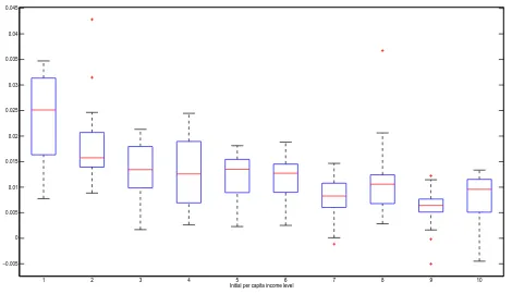
−0.005 0 0.005 0.01 0.015 0.02 0.025 0.03 0.035 0.04 0.045

1 2 3 4 5 6 7 8 9 10

Initial per capita income level

Per capita income growth

Figure 2:Boxplot of per capital income growth

the response of the dependent variable is very different for different groups of initial income and, therefore, justifies the application of quantile regressions to analyze convergence.

(14)

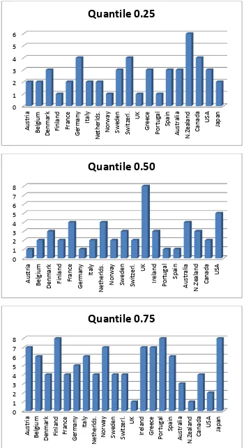
0

Figure 3:Histogram of distribution of countries by quantiles

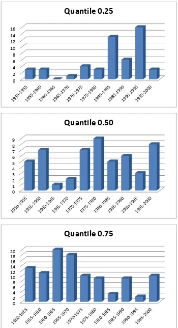
includes the highest rates of growth, is represented by two consecutive periods, 1960–1965 and 1965–1970.

(15)

0

Figure 4:Histogram of distribution of periods by quantiles

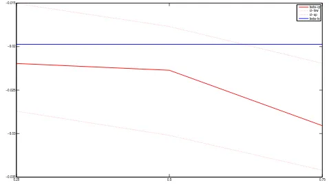
Table 1:Estimation of panel quantile regression

(16)

0.25 0.5 0.75 −0.028

−0.026 −0.024 −0.022 −0.02 −0.018 −0.016 −0.014 −0.012 −0.01

beta−qr ci−low ci−up beta−ls

Figure 5:Estimation of panel quantile regression. Fixed effects by countries

0.25 0.5 0.75

−0.035 −0.03 −0.025 −0.02 −0.015

beta−qr ci−low ci−up beta−ls

Figure 6:Estimation of panel quantile regression. Fixed effects by periods

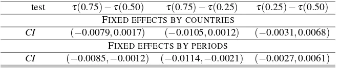
As we can see in Table 2, although the respective tests of equality between quantiles are not rejected when we consider fixed effects by countries, these out-comes imply, at least, a slightly greater speed of convergence between the countries that belong to the upper quantiles. This result helps us to explain the existence of different clubs that converge at different rates. Finally, when testing the equality of the beta parameters for the different quantiles, we reject the null of the beta parameter for the highest quantile, τ(0.75), being equal to the lowest, τ(0.25), when considering fixed effects by periods. This means that the convergence speed is significantly different for 1980-1985 and 1990–1995, the periods mostly represented in the first quantile, than for 1960–1965 and 1965–1970, the periods that represented the upper quantile. These results inform us that absolute convergence in the OECD is a phenomenon driven by a set of countries and that it was concentrated during the years 1960 to 1970.

(17)

Table 2:Tests of quantiles

test τ(0.75)−τ(0.50) τ(0.75)−τ(0.25) τ(0.25)−τ(0.50)

FIXED EFFECTS BY COUNTRIES

CI (−0.0079,0.0017) (−0.0105,0.0012) (−0.0031,0.0068)

FIXED EFFECTS BY PERIODS

CI (−0.0085,−0.0012) (−0.0114,−0.0021) (−0.0027,0.0061)

process is mainly due to the countries belonging to the upper quantile, which is not represented by USA, a country considered as the leader in other studies such as those of Bentzen (2005), Greasley and Oxley (1998) and Datta (2003). This result also contradicts the idea of Epstein et al. (2003) that the convergence in this set of countries is mainly due to the performance of the countries that grew less. Focusing on periods, our outcomes confirm those of Datta (2003) who finds convergence during the period 1950–1992 although with a cyclical trend, and modify the results of Mello and Perrelli (2003) who found a lower degree of convergence during the period 1960–1985. Our analysis, however, shows that convergence was stronger in the period 1960–1970. The differences between this study and that of Mello and Perrelli may be due to the fact that the did not perform a quantile regression with panel data and, therefore, cannot distinguish between fixed and time effects. Futhermore, this period of higher convergence, located between 1960–1970, shows a rate of about 3 per cent, higher than that obtained when the model is estimated by OLS and that obtained in previous analyses, of about 2 per cent.

The period after the Second World War is known as the Golden Age, and runs from 1950 to 1973. Its analysis has attracted a considerable amount of attention from economists and historians looking for the causes of the intense growth of the world (and, especially the European economy). Authors as relevant as Maddison (1959, 1995), Toniolo (1998), Crafts (2007) and Prados de la Escosura (1993), among others, provide the main ingredients of the virtuous circle that sustained the Golden Age: high investment rates were instrumental in the transfer of technology; exports promoted the expansion of markets, abundant labour and an adequate stock of human capital, apt institutions and good policies. All of these factors helped the poorest countries to record higher growth rates than the richest, especially after 1960, thus producing an inevitable process of catch-up, that is, of conditional convergence. The results of this paper confirm these studies by indicating how the convergence found in this period is represented by countries that were the poorest but that grew faster (those that belong to the upper quantile).

(18)

methodology, the panel quantile regressions model, are in line with the stylized facts highlighted by the historiography.

4 Conclusions

The idea underlying the concept of convergence, based on the neoclassical theory, is that, given the existence of decreasing returns in the use of capital and assuming equality of preferences and technology, countries which begin with lower levels of income per capita will tend to grow more quickly.

Empirical issues have played a key role in the literature on convergence using different kinds of data and different estimations to test the hypothesis. Nevertheless, the outcomes they obtain lead to different conclusions. In general, the hypothesis of convergence is accepted with cross-sectional data but it is rejected if the time-series methodology is used. Other approximations that apply other methods such as the Kalman filter and the Kernel density function do not help to clarify the issue.

In the preceding sections, we have reviewed the results of a number of these empirical studies of convergence among the OECD countries and discussed some limitations of these works. This paper attempts to deal with them by presenting a new and more appropriate methodology, quantile regressions. With this methodology, we are able to observe the existence of different steady states where a set of countries converge during a certain time. The results obtained with this specification support the view that absolute convergence in the OECD is a phenomenon driven by a set of countries, those belonging to the upper quantile, which mainly occurred during the 1960s.

Acknowledgements: The authors benefited from the helpful comments made by two

anonymous referees; this version owes much to them. The authors are very grateful to the

financial support of theMinisterio de Ciencia y Tecnologíaunder grant ECON2008-03040

(19)

References

Alesina, A., and R. Perotti (1996). Income Distribution, Political Instability and Investment.European Economic Review40(6), 1203–1228.

http://www.sciencedirect.com/science/article/pii/0014292195000305

Barro, R.J., and X. Sala-i-Martín (1995).Economic Growth. McGraw-Hill.

Barro, R. (1991). Economic Growth in a Cross Section of Countries. Quarterly

Journal of Economics106(2), 407–443.

http://academic.oup.com/qje/article/106/2/407/1905452/Economic-Growth-in-a-Cross-Section-of-Countries

Baumol, W.J. (1986). Productivity Growth, Convergence and Welfare: What the Long Data Show.American Economic Review76(5), 1155–1159.

https://ideas.repec.org/a/aea/aecrev/v76y1986i5p1072-85.html

Bentzen, J. (2005). Testing for Catching-up Periods in Time-Series Convergence.

Economics Letters88(3), 323–328.

http://www.sciencedirect.com/science/article/pii/S0165176505001345

Bernard, A. and S. Durlauf (1995). Convergence in International Output.Journal of

Applied Econometrics10(2), 97–108.

http://onlinelibrary.wiley.com/doi/10.1002/jae.3950100202/abstract

Bernard, A. and S. Durlauf (1996). Interpreting Test of the Convergence Hypothesis.

Journal of Econometrics71(1), 161–173.

Crafts, N. (2007). European Growth in the Age of Regional Economic Integration: Convergence Big Time? Background paper, Reshaping Economic Geography.

Datta, A. (2003). Time-series Test of Convergence and Transitional Dynamics.

Economics Letters81(2), 233–240.

De la Fuente, A. (1997). The Empirics of Growth and Convergence: A Selective Review.Journal of Economics Dynamics and Control21(1), 27–73.

Dickey, D.A. and W.A. Fuller (1979). Distribution of the Estimators for Autorregres-sive Time Series with a Unit Root.Journal of the American Statistical Association

74(366), 427–431.

(20)

Dickey, D.A. and W.A. Fuller (1981). Likelihood Ratio Statistics for Autorregresive Time Series with a Unit Root.Econometrica49(4), 1057–1072.

https://www.jstor.org/stable/1912517

Dollar, D. (1992). Outward-Oriented Developing Economies Really Do Grow More Rapidly: Evidence from 95 LDCs, 1976–1985.Economic Development and

Cultural Change40(3), 523–544.

Durlauf, S.N., and P.A. Johnson (1995). Multiple Regimes and Cross-Country Growth Behaviour.Journal of Applied Econometrics10(4), 365–384.

http://onlinelibrary.wiley.com/doi/10.1002/jae.3950100404/abstract

Epstein, P., P. Howlett, and M.S. Schulze (2003). Distribution Dynamics: Strat-ification, Polarization and Convergence among OECD Economies,1870–1992.

Explorations in Economic History40(1), 78–97.

Fischer, S. (1993). The Role of Macroeconomic Factors in Growth. Journal of

Monetary Economics32(3), 485–512.

http://www.sciencedirect.com/science/article/pii/030439329390027D

Greasley, D. and L. Oxley (1998). A Tale of Two Dominions: Comparing the Macroeconomic Records of Australia and Canada since 1870.Economic History

Review51(2), 294–318.

http://onlinelibrary.wiley.com/doi/10.1111/1468-0289.00092/pdf

Im, K.S., M.H. Pesaran and Y. Shin (2003). Testing for Unit Roots in Heterogeneous Panels.Journal of Econometrics115(1), 53–74.

Islam, N. (1995). Growth Empirics: A Panel Data Approach.Quarterly Journal of

Economics110(4), 1127–1170.

http://www.jstor.org/stable/2946651

Koenker, R. (2004). Quantile Regression for Longitudinal Data. Journal of Multivariate Analysis91(1), 74–89.

http://www.sciencedirect.com/science/article/pii/S0047259X04001113

Koenker, R., and J. Machado (1999). Goodness of Fit and Related Inference Processes for Quantile Regression. Journal of American Statistical Association

94(448), 1296–1310.

(21)

Lamarché, C. (2010). Robust Penalized Quantile Regression Estimation for Panel Data.Journal of Econometrics157(2), 396–408.

Levin, A., C.F. Lin, and C. Chu (2002). Unit Roots Tests in Panel Data: Asymptotic and Finite-Sample Properties.Journal of Econometrics108(1), 1–24.

Lucas, R.E, (1988). On the Mechanics of Economic Development. Journal of

Monetary Economics22(1), 3–42.

Lucas, R.E. (1990). Why doesnt Capital Flow from Rich to poor Countries? The

American Economic Review80(2), 92–96.

https://www.econ.nyu.edu/user/debraj/Courses/Readings/LucasParadox.pdf

Maddison, A. (1959). Economic Growth in Western Europe. Banca Nazionale del Lavoro Quarterly Review, 58–102.

Maddison, A. (1995).Monitoring the World Economy, 1820–1992. Paris.

Mankiw, G.N., D. Romer, and D.N. Weil (1992). A Contribution to the Empirics of Economic Growth.The Quarterly Journal of Economics107(2), 407–437. https://academic.oup.com/qje/article/107/2/407/1838296/A-Contribution-to-the-Empirics-of-Economic-Growth

Mello, M., and R. Perrelli (2003). Growth Equations: A Quantile Regression Exploration. The Quarterly Review of Economics and Finance, 43(4), 643–667. http://www.sciencedirect.com/science/article/pii/S1062976903000437

Nahar, S., and B. Inder (2002). Testing Convergence in Economic Growth for OECD Countries. Applied Economics34(16), 2011–2022.

http://www.tandfonline.com/doi/pdf/10.1080/00036840110117837

Perron, P. (1989). The Great Crash, the Oil Price Shock, and the Unit Root Hypothesis.Econometrica57(6), 1361–1401.

(22)

Quah, D.T. (1993). Empirical Cross-Section Dynamics in Economic Growth.

European Economic Review37(2-3), 426–434.

http://www.isid.ac.in/ tridip/Teaching/DevEco/Readings/02Convergence/06Quah-EER1993.pdf

Quah, D.T. (1996). Twin Peaks: Growth and Convergence in Models of Distribution Dynamics. Economic Journal106(437), 1045–1055.

Quah, D.T., (1997). Empirics for Growth and Distribution: Stratification, Polariza-tion, and Convergence Clubs.Journal of Economic Growth2 (1), 27–59.

Ram, R. (2008). Parametric Variability in Cross-Country Growth Regressions: An Application of Quantile-Regression Methodology.Economics Letters99(2), 387–389.

Rassek, F., M.J. Panik, and B.R. Kolluri (2001). A Test of the Convergence Hypoth-esis: The OECD Experience, 1950-1990. International Review of Economics & Finance10(2), 147–157.

http://www.sciencedirect.com/science/article/pii/S105905600100079X

Romer, P.M. (1986). Increasing Returns and Long Run Growth.Journal of Political

Economy94(5), 1002–1037.

Romer, P.M. (1990). Endogenous Technological Change. Journal of Political Economy98(5, part. 2), 71–102.

http://pages.stern.nyu.edu/ promer/Endogenous.pdf

Sala-i-Martín, X.(1996). The Classical Approach to Convergence Analysis.

Eco-nomic Journal106(437), 1019–1036.

Toniolo, G., (1998). Europes Golden Age, 1950-1973: Speculations from a Long Term Perspective.Economic History Review51(2), 252–267.

Zivot, E. and D.W.K. Andrews (1992). Further Evidence on the Great Crash, the Oil-price Shock and the Unit Root Hypothesis. Journal of Business & Economics Statistics10(3), 251–270.

(23)

Please note:

You are most sincerely encouraged to participate in the open assessment of this article. You can do so by posting comments.

Please go to:

http://dx.doi.org/10.5018/economics-ejournal.ja.2017-4

The Editor