Mathematics and Informatics ICTAMI 2005 - Alba Iulia, Romania
STABILITY ANALYSIS OF SHALLOW WAKE FLOWS WITH FREE SURFACE
Sergejs Nazarovs
In particular, neglecting of the momentum correction coefficients may lead to a systematic bias that underestimates critical transition values marking the boundary of instability.
2000 Mathematics Subject Classification: Applied Mathematics.
1. Introduction
Wake flows (flows behind obstacles, such as islands) are considered shal-low if the transverse scale of the fshal-low is much larger than the vertical scale (water depth). Experiments show that limited water depth has a strong in-fluence on the development of flow instabilities. In particular, evolution of three-dimensional instabilities is prevented due to small vertical scale, but transverse growth of perturbations is hampered by bottom friction. As a re-sult, development of wakes in shallow water is different from the ones in deep water.
However, vortex structures observed in shallow water in many cases re-semble very much flow patterns in deep water. For example, photograph Nr. 173 by Van Dyke [6] shows formation of eddies organized into a vortex street behind an obstacle in shallow water although the Reynolds number for this case is 107 [6]. Note that vortex street pattern in unbounded flows is limited to much smaller Reynolds numbers.
The stability of shallow flows has been analyzed in literature both experi-mentally and theoretically [1], [2], [3], [5]. Two main assumptions are usually being made in order to facilitate the analysis under the shallow water model. The essence of the first assumption is that the free surface of the flow is not perturbed and acts as ”rigid-lid” (so-called ”rigid-lid” assumption). Accord-ing to the second assumption, the velocity is supposed to be independent on vertical coordinate. This assumption results from the fact that the governing equations for shallow flow are the depth-averaged.
In some cases, however, the two assumptions may not be appropriate. Fluc-tuations of bottom friction coefficient and changes in flow geometry can result in appreciable deviation of the real flow from above-mentioned assumptions. In order to take into account the non-uniformity of velocity distribution, mo-mentum correction coefficients were applied by several authors [8], [9].
paper in order to evaluate influence of non-uniformity of velocity distribution. The stability of the flow is analyzed for various values of the momentum correc-tion coefficients. The Froude number is used in order to evaluate the influence of ”rigid-lid” assumption on stability characteristics of shallow flows.
2.Problem Formulation
The governing equations for shallow flow can be obtained by integrating Euler equations with respect to vertical coordinate and have the form
∂h ∂t +
∂
∂x(uh) + ∂
∂y(vh) = 0 (1) ∂u
∂t + (2β1−1)u ∂u
∂x + [(β1−1) u2
h +g] ∂h
∂x + (β2 −1)u ∂v ∂y+ +(β2−1)uv
h ∂h ∂y +β2v
∂u
∂y −Sox+
cfu√u2 +v2
2h −F(y) = 0 (2) ∂v
∂t +β2u ∂v
∂x + (β2−1)v ∂u
∂x + (β2−1) uv
h ∂h
∂x + (2β3−1)v ∂v ∂y+ +[(β3−1)v
2
h +g] ∂h
∂y −Soy +
cfv√u2+v2
2h = 0 (3)
wherexandyare spatial coordinates,tis time,uandv are depth-averaged velocity components in thexand y directions respectively,his water depth,g is acceleration due to gravity,F(y) is the forcing function,S0x=−∂zb(x, y)/∂x and S0y = −∂zb(x, y)/∂y are the bed slopes, zb is distance from the bottom, cf is the friction coefficient defined by the equation
1
√cf =As+Bsln(R√cf)
whereAs andBs are coefficients defined in [7]. Shear stress at the boundary is modelled by the Chezy formulaτwx= 1
2cfρu √
u2+v2andτwy = 1 2cfρv
√
u2+v2, whereρ is density, τwx and τwy are wall shear stresses along thexand y direc-tions respectively.
β1 = 1 hU2
Z z2
z1
u2dz (4)
β2 = 1 hU V
Z z2
z1
uvdz (5)
β3 = 1 hV2
Z z2
z1
v2dz (6)
where u and v are velocity components, but U and V are depth-averaged velocity components in the x and y directions respectively.
Introducing characteristic length b and the characteristic velocity U0, we choose the measure of time in the form b/U0. Rewriting the equations in dimensionless form, we obtain:
∂hd ∂td +
∂
∂xd(udhd) + ∂
∂yd(vdhd) = 0 (7) ∂ud
∂td + (2β1−1)ud ∂ud
∂xd + (β1 −1) u2 d hd ∂hd ∂xd + 1 F r2
∂hd
∂xd +β2vd ∂ud ∂yd+ (β2−1)ud∂vd
∂yd + (β2−1) udvd
hd ∂hd ∂yd +
cfudqu2 d+vd2
2hd −F˜(yd) = 0 (8) ∂vd
∂td +β2ud ∂vd
∂xd + (β3−1) v2 d hd ∂hd ∂yd + 1 F r2
∂hd
∂yd + (β2−1)vd ∂ud ∂xd+ (β2−1)udvd
hd ∂hd
∂xd + (2β3−1)vd ∂vd ∂yd +
cfvdqu2 d+v2d
2hd = 0 (9)
where ud = u/U0, td = tU0/b, xd = x/b, hd = h/H0, yd = y/b, ˜F(yd) = bF(yd)/U02, H0 is undistributed water depth andF r is Froude number, repre-senting the ratio of inertia and gravity forces, that is defined by the expression F r=U0/√gH0.
Dropping the subscript ”d”, we seek a perturbed solution for equations (7-9) in the form:
u = U(y) + ˆu(y)e−λt+ikx (10)
v = ˆv(y)e−λt+ikx (11) h = H0
b + ˆh(y)e
where k is a wavenumber andλ=λr+iλi is a complex eigenvalue.
Substituting (10-12) into (7-9), and performing linearization in the neigh-borhood of the base flow, we obtain a system of ordinary differential equations:
H0
b ikuˆ+ikUˆh+ H0
b dˆv
dy −λˆh= 0 (13)
[(2β1−1)ikU+sU]ˆu+[(β1−1)ikU 2b
H0 + ik F r2−
sU2b
2H0 ]ˆh+(β2−1)U dˆv
dy+β2vUy−λuˆ= 0 (14) 1
F r2 dhˆ
dy + (ikβ2U + s
2U)ˆv−λˆv = 0 (15) with the boundary conditions
v(±∞) = 0 (16)
where s= cfb
H0,u=u(y), v =v(y) andh=h(y).
3.Solution Method
Using a substitution x= 2
πarctan(y); y∈(−∞; +∞);x∈[−1; 1],
we represent the functions v(x),u(x) andh(x) in the form of fundamental interpolation polynomials: u(x) = n X k=1 ak Tn(x) (x−xk)T′
n(xk) (17) v(x) = n X k=1
bk(1−x 2) (1−x2
k)
Tn(x) (x−xk)T′
n(xk) (18) h(x) = n X k=1 ck Tn(x) (x−xk)T′
n(xk)
(19) whereak,bk andckare unknown constants, butTn(x) is ann-order Cheby-shev polynomial that has the form Tn(x) = cos(n ∗arccos(x)). The points xk, defined by the expression xk = cos(2k−1)π
Tn(x)
(x−xk)Tn′(xk)) is equal to zero, ifx=xj, where xj is a zero of ann-order
Cheby-shev polynomial, and j 6=k. If x=xk then using the Taylor series expansion of Tn(x) about the point x=xk we obtain:
Tn(x) (x−xk)T′
n(xk))
= Tn(xk) + (x−xk)T
′
n(xk) +
(x−xk))2
2 Tn′′(xk)+< ... > (x−xk)T′
n(xk)
= = 1 + (x−xk)
2 T′′
n(xk) T′
n(xk)
+< ... >(20) Hence
Tn(x) (x−xk)T′
n(xk)) =
0, if x=xj, j
6
=k
1, if x=xj, j =k (21)
Using the collocation method and choosing zeroes of Chebyshev polynomi-als as the collocation points we obtain
(A−λB)d= 0 (22)
where A and B are two complex-valued matrices. Vector d has the form d=a1, a2, ..., an, b1, b2, ..., bn, c1, c2, ..., cn
Solving the generalized eigenvalue problem (22), for givensandkwe obtain a set of eigenvalues λ.
The real parts of eigenvalues λ determine linear stability of the base flow. The flow is said to be linearly stable, if real parts of allλare positive. If the real part of the eigenvalue λ of at least one mode is negative then a perturbation grows exponentially with time and the flow is said to be linearly unstable. Numerical methods can be used in order to find for a given wavenumber k a value of s, for which one mode has λr equal to zero, while all other λ have positive real parts. That enables to build the neutral stability curve, that is defined as a set of points in the (k,s)-plane for which one λ has the real part equal to zero, while real parts of all other λ are positive. The critical value, sc of the parameter s is defined as the coordinate of the highest point of the curve, or sc =max(s(n)(k)).
The sc parameter is very important in linear stability analysis. The flow is stable for allk if the value ofs is higher thansc, and flow is unstable for some k if s < sc.
This paper presents an attempt to evaluate the influence of ”rigid-lid” assumption and momentum correction coefficients on the value ofscparameter. The rigid-lid assumption is evaluated by solving problems (13-15) numerically for different values of Froude number as well as b/H0 parameter that is the ratio of the characteristic width of the wake and water depth and comparing the critical values, sc, of the parameters. The assumption of uniform velocity distribution across the vertical coordinate is evaluated by solving problems (13-15) for different values of momentum correction coefficients β1 and β2.
The values of sc have been calculated for the following values of the pa-rameters F r,b/H0, β1, and β2:
F r = 0.0001,0.1,0.2. b/H0 = 5,50.
β1 = 1.00,1.05,1.10. β2 = 1.00,1.05,1.10.
The critical values of the stability parameter for finite Froude number F r and various values of parameterb/H0 are compared with those obtained under ”rigid-lid” assumption by Kolyshkin&Nazarovs [4].
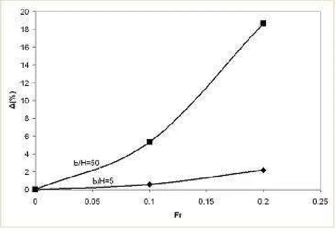
The results (in terms of percentage difference) are shown in Figure 1.
The two values of the parameter b/H0 are chosen since the condition b/H0 ≫1 is consistent with the shallow water approximation. It is seen that although the stability boundary is quite sensitive to variations of Froude num-ber, the error in determining the sc parameter is below 6% if Froude number is less than 0.2 for the case b/H0=5, and if the Froude number is less than 0.1 for the case b/H0=50. The Froude number F rH (based on the undisturbed water depth) is related to F r by means of the formulaF rH =F rqb/H0. The parameterF rH for real island wakes is in the range 0.1-0.2. So, the ”rigid-lid” assumption is precise enough for calculation of the sc parameter for the range of Froude numbers typical for shallow flows.
has, in its turn, stabilizing effect on the flow, but its influence diminishes with the growth of β1. Unfortunately, the values of coefficients β1 and β2 for real island wakes are not known. However as the error in determining the sc parameter may grow with increased values ofβ1 (the stability boundary can be underestimated with increase ofβ1) it might be important to know the values of β1 and β2 for analyzed shallow flows.
References
[1] Chen, D., Jirka, G. H., Absolute and convective instabilities of plane turbulent wakes in a shallow water layer., Journal of Fluid Mechanics., v 338., 1997., pp. 157-172.
[2] Falques, A., Iranzo, V., Numerical simulation of vorticity waves in the nearshore., Journal of Geophysical Research., v. 99., 1994., pp. 825 - 841.
[3] Ghidaoui, M., Kolyshkin, A. A. Linear stability analysis of lateral mo-tions in compound open channels., Journal of Hydraulic Engineering., v. 125, 1999., pp. 871 - 880.
[4] Kolyshkin, A., Nazarovs, S., On the stability of wake flows in shallow water., Abstracts of 10thInternational Conference on Mathematical Modelling and Analysis., Matematikos ir Informatikos Institutas., 2005., p. 83.
[5] Sokolofsky, S. A., Carmer, C., Jirka G. H., Shallow turbulent wakes: linear stability analysis compared to experemental data., Shalow flows., A. A. Balkema Publishers., 2003.
[6] Van Dyke, M., An album of Fluid Motion., The Parabolic Press., 1982. [7] Wylie, E. B., Bedford, W. K., Streeter, V. L., Fluid Mechanics., Ninth Edition., Mc-Graw Hill., 1998., p. 288.
[8] Xia, R., Yen, B. C., Significance of averaging coefficients in open-channel flow equations., Journal of Hidraulic Engineering., v. 120., 1994., pp. 169 -189.
[9] Yen, B. C., Open-channel flow equations revisited., Journal of the engi-neering mechanics division., v. 99., 1973., pp. 979 - 1009.
S. Nazarovs
Institute of Engineering Mathematics Riga Technical University