Breaz Nicoleta. 122KB Jun 04 2011 12:08:27 AM

NUMERICAL EXPERIMENTS WITH LEAST SQUARES

SPLINE ESTIMATORS IN A PARAMETRIC REGRESSION

MODEL

by Nicoleta Breaz

Abstract. In this paper, we discuss two aspects regarding the least squares estimators in a parametric regression model. First, we make a numerical experiment that emphasizes the goodness of the least squares spline fit with respect to the polynomial fit. For the second goal of the paper, we implement a CV-based knots selection algorithm in Matlab 6.5 environment and we apply it on some test function, in order to analyse how the CV method works, in the knots selection for the least squares spline estimators.

1. Introduction

We consider the regression model,

( )

+ε

= f X

Y ,

with X, Y, two random variables and ε , the error term. After a sampling, we obtain the observational model,

( )

+ ,i=1,n

= i i

i f x

y ε

and we suppose that ε =

(

ε₁,ε₂,...,ε_n

)

′~N

(

0,σ2I

)

.

If we assume that f has some parametric form, well defined except from a finit number of unknown coefficients, then we are in the parametric regression setting.

One of the most used regression models is the polynomial regression, that is

i q i q i

i

i x x x

y =α₀ +α₁ +α₂ 2 +...+α +ε .

explicative variables, X,X2,...,Xq. But before make this estimation it is necessary to establish the form of the regression function, or more precisely, in this case, the polynomial’s degree. An ordinary solution to this problem is to estimate the model, for different values of q and then, to compare these models, by performing a regression analysis, either by graphical comparison and/or by quantitative methods (see [7], [8], [9]).

As an alternative, there exists some data driven selection methods that give the appropriate value for q (see [4] and [8]). One of such methods is the cross validation method (CV). Based on this method, the optimal degree q will be that which minimizes the cross validation function,

( )

(

( )

( )

)

2

1 1

∑

_{= −} −

= n

i

i i q i f x

y n q

CV ,

where fq( )i

− _{is the regression polynomial, fitted from all data, less the i-th data.}

A leaving-out-one resampling method is used here. We obtain the fitted models, f_q( )−i , i=1,n, from n learning samples (each one, with n-1 data), then we validate these models by other n test samples, formed with the one-left-out data.

We already discussed in [2] and [3], how the CV method works, in the case of degree selection, for the polynomial regression and in the case of smoothing parameter selection, for the smoothing spline regression, respectively.

Also, in [2], we proposed a combined algorithm for degree selection, in the case of the polynomial regression. This algorithm is based either on the CV method and on the regression analysis techniques.

Degree selection algorithm

Step 1. Simulate a sample data,

(

xi,yi

)

,i=1,n and if it is necessary, order and weight the data, with respect to the data sites, xi.

Step 2. For these simulated data, find a sample with p replicate values of qCV and the related distribution.

Step 4. If the fit with the q1CV degree polynomial is validated by both graphical and quantitative regression analysis, Stop.

Else, follow the next step.

Step 5. Make the regression comparative analysis for the cases 1

CV

q , 2 CV

q ,

1

1 − CV

q , q_CV1 +1 and establish the optimal fitting. Stop.

However, on wide data range, the polynomial regression works only as a local approximation method, leading to the necesity of finding a more flexible model. A solution to this problem could be the statement of a polynomial regression problem, on each subinterval from a partition of the data range, dealing with a switching regression model, that bears structural changes in some data points.

In this way, the polynomial spline functions, with their great flexibility, arise as good estimators in such cases. We remind here that a polynomial spline function of m degree, defined with respect to a mesh,

∞ ≤ < < < < < ≤ −∞

∆: a t₁ t₂ ... t_N b , is a piecewise polynomial function (the breaks or the function knots are t_k ,k =1,N), with the pieces joined at the knots, so that the function has m-1 continuous derivatives (see [5] and [6]).

Thus, if we use the truncated power functions (see [5]), then we can write for a parametric spline regression model, the form

(

)

ε β α + − + = ₊ = =

∑

∑

m k N k k m k k

kX X t

Y

1 0

.

This model can be estimated with the least squares method, after a reduction to a multiple linear model, namely,

N N m

mZ U U

Z

Y =α₀ +α_{1 1} +...+α +β_{1 1}+...+β ,

with the explicative variables given by

(

)

,k 1,N. U , m 1, k ,

k = − =

The resulted estimator of the regression function is called the least squares spline estimator.

Here, likewise in the polynomial regression, we have to estimate first, the degree of function, the number of knots and the location of its.

Selection of the degree m is usually made as a result of a graphical analysis of data and selection of the knots number, N, depends on the desired amount of flexibility. Also, there are several elementary rules for selecting the knots. Thus, for a linear spline, the knots are placed at the points where the data exhibit a change in slope, and for a quadratic or cubic spline, the knots are placed near local maxima, minima, or inflection points in the data.

Besides these settings, there are also data driven methods for selecting these parameters (see [1] and [4]). One of such methods and also, a comparison between polynomial and spline regression, follow in the next sections.

2. CV-based best polynomial fitting

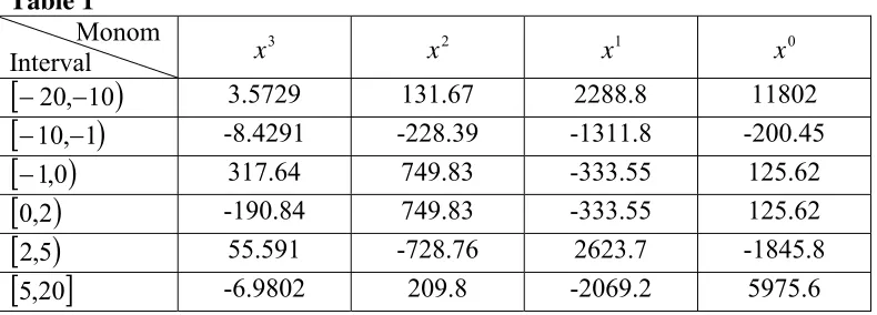
For all numerical experiments which will be made in this paper, we consider as a test function, a piecewise function, f :

[

−20 ,20

]

→, formed by six pieces of cubics, having the breaks –10, -1, 0, 2, 5 and the coefficients given in the following table:

Table 1

Monom Interval

3

x x2 x1 x0

[

−20,−10

)

3.5729 131.67 2288.8 11802

[

−10,−1

)

-8.4291 -228.39 -1311.8 -200.45

[

−1,0

)

317.64 749.83 -333.55 125.62

[

0,2

)

-190.84 749.83 -333.55 125.62

[

2,5

)

55.591 -728.76 2623.7 -1845.8

[ ]

5,20 -6.9802 209.8 -2069.2 5975.6 [image:4.595.109.504.385.527.2]

( )

+ , =1,50

= f x i

y_{i i} ε_i ,

where ε_i’s come from a random number generator simulating independently and identically distributed, ε_i ~ N

(

0,500

)

, random variables.

For these data, we start with a polynomial fitting. In order to establish the appropriate degree, we have used the degree selection algorithm, reminded in the introductory section of this paper. For 100 replicates of the experiment, the following distribution of the degree q_CV is obtained:

    13 85 1 1 0 0 0 7 6 5 4 3 2 1 : CV q .

Now, applying the second part of the algorithm, we will reduce the problem of the optimal degree polynomial fitting to a comparison with the regression analysis techniques, between the mode of the distribution, qCV =6, and the cases 5qCV = and qCV =7. We will not present here the graphical comparison, but we mention that the curves for qCV =6 and qCV =7 have almost the same behaviour with respect to the data, being more appropriate than the curve for q_CV =5. The quantitative analysis also recommends the case

6

=

CV

q , in spite of the other cases. For example the adjusted squared R has the values

(

5

)

0,940 2

= =

q

R ,

(

6

)

0,946 2

= =

q

R ,

(

7

)

0,947 2

= =

q

R .

Hence, we state that the CV-based best polynomial estimator with respect to these data is the sixth degree polynomial.

Anyway, the 95%-confidence bounds presented below show that the accuracy of the best polynomial estimation is not very good (see the magnitude of the confidence interval for the coefficients a₆, a₅, a₄):

6

a = 40,27 (-426,6; 507,1),

4

a = 14,53 (0,911; 28,16), 3

a = -1,034 (-1,786; -0,2822), 2

a = -0,1757 (-0,2656; -0,08582), 1

a = 0,002335 (0,000746; 0,003924), 0

a = 0,0001942 (3,79e-005; 0,0003506).

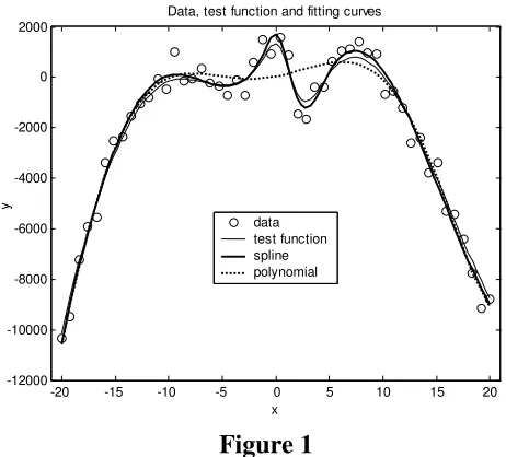
3. Least squares spline fitting versus polynomial fitting

In order to emphasize the quality of the spline estimator, with respect to that of the polynomial estimator, we have fitted the same data with a cubic spline function (of third degree), having as knots of multiplicity 1, the breaks of the test function, namely, -10, -1, 0, 2, 5 and the end knots, -20, 20, of multiplicity 4. In this regard, for illustrate the goodness of spline fitting against the best degree polynomial fitting, we have plotted in the following figure, these two fittings, together with the test function and the data.

-20 -15 -10 -5 0 5 10 15 20

-12000 -10000 -8000 -6000 -4000 -2000 0 2000

Data, test function and fitting curves

x

y

[image:6.595.183.414.315.524.2]

data test function spline polynomial

Figure 1

4. CV-based knots selection in the least squares spline regression

Simillary with the polynomial case, we propose here a data driven method for the selection of the least squares spline knots, based on a CV-like function,

( )

∑

(

( )

( )

)

=

− −

= n

i

i i i

N y f x

n CV

N

1

2

1

λ

λ .

In this expression, ( )i

N

f_λ− is the least squares spline estimator, with the knots given by λ_N =

{

t₁,t₂,...,t_N

}

, obtained by leaving out the i-th data from the sample. The optimal set of knots, λˆ_Nˆ, will be derived by minimizing, for fixed

N, the expression CV

( )

λ_N , thus resulting the estimator λˆ and then , by _N obtaining λˆ_Nˆ, with Nˆ the minimizer of CV

( )

λˆN . A weighted version of this function (the generalized cross validation function, see [4]) was already used in this regard.

In order to show how this method works, we implemented the following CV-based algorithm in the Matlab 6.5 environment.

Knots selection algorithm

Step 1. Read the data

(

x_i,y_i

)

, i=1,n.

Step 2. For various sets of knots, determine the least squares fitting spline,

( )i

N f_λ− .

Step 3. For the cases considered in the previous step, calculate CV

( )

λN .

Step 4. Determine λCV_N , for which

( )

( )

N

CV

N CV

CV

N λ

λ =min_λ .

Stop.

We run this algorithm on the same simulated data as in the previous sections. Starting with the information contained in the shape of the observed data curve (see figure 1), we choose m=3 as the degree of the spline estimator. As competitors, we propose the following four sets of knots:

S2={-20, -10, -1, 0, 2, 5, 20},

S3={-20, -20, -20, -20, -10, -1, 0, 5, 20, 20, 20, 20},

S4={-20, -20, -20, -20, -11, -2, 0, 1, 4, 20, 20, 20, 20}.

The first set is that which was used in the previous section. With respect to the first set, the second set gives up to the multiplicity of the end knots and the third to the knot t=2. The last set is choosed according to the elementary rools, reminded in the introductory section. Thus, we place the knots near local minima, maxima or inflection points in the data. Certainly, our expectations on the optimal knots are for the first set, this set being actualy formed with the breaks of the test function.

In what follows, we will see if the proposed CV-based algorithm can selects the optimal knots. For 100 replicates of the algorithm, with different seeds of the random number generator, we obtain the following mean values of the cross validation function, CV

( )

λ_N , corresponding to the four sets of knots:

314914,756972, 13638912,940932, 620668,166187, 389896,095517.

It can be observed that the first set of knots, S1 (the breaks of the test

function), followed by the sets S4, S3, S2 (in this order), is that selected by the

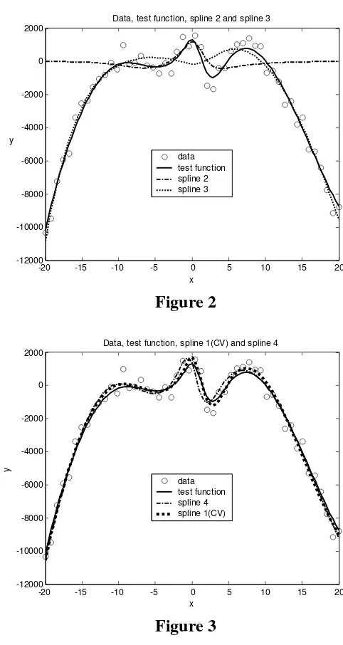
CV method. As the following plots show, this hierarchy is validated also by the graphical comparison of these four spline fits. For the clarity of the pictures sake, we plot in the first figure, the cases S3, S2 and in the second figure, the

-20 -15 -10 -5 0 5 10 15 20 -12000

-10000 -8000 -6000 -4000 -2000 0 2000

Data, test function, spline 2 and spline 3

y

[image:9.595.174.415.80.533.2]

x data test function spline 2 spline 3

Figure 2

-20 -15 -10 -5 0 5 10 15 20

-12000 -10000 -8000 -6000 -4000 -2000 0 2000

x

y

Data, test function, spline 1(CV) and spline 4

data test function spline 4 spline 1(CV)

Figure 3

We can see that the curves from the first figure fit he data poorly, while the curves from the last figure, indicate good fits. Anyway, the better is the curve corresponding to the set S1. Therefore, the cross validation method selects the

References

[1].de Boor C., A Practical Guide to Splines, Springer-Verlag, New York, 1978 [2].Breaz N., The cross-validation method in the polynomial regression, Acta Universitatis Apulensis, Mathematics-Informatics, Proc. of Int. Conf. on Theory and Appl. of Math. and Inf., Alba Iulia, no. 7, Part B, 67-76, 2004 [3].Breaz N., The cross-validation method in the smoothing spline regression, Acta Universitatis Apulensis, Mathematics-Informatics, Proc. of Int. Conf. on Theory and Appl. of Math. and Inf., Alba Iulia, no. 7, Part B, 77-84, 2004 [4].Eubank R.L., Nonparametrc Regression and Spline Smoothing-Second Edition, Marcel Dekker, Inc., New York, Basel, 1999

[5].Micula Gh., Funcţii spline şi aplicaţii, Editura Tehnică, Bucureşti, 1978 [6].Micula Gh., Micula S., Handbook of Splines, Kluwer Academic Publishers, Dordrecht-Boston-London, 1999

[7].Saporta G., Probabilités, analyse des données et statistique, Editions Technip, Paris, 1990

[8].Stapleton J.H., Linear Statistical Models, John Wiley & Sons, New York-Chichester-Brisbane, 1995

[9].Tassi Ph., Méthodes statistiques, 2e édition, Economica, Paris, 1989

Author: