On: 26 Sept em ber 2013, At : 00: 04 Publisher : Rout ledge
I nfor m a Lt d Regist er ed in England and Wales Regist er ed Num ber : 1072954 Regist er ed office: Mor t im er House, 37- 41 Mor t im er St r eet , London W1T 3JH, UK
Accounting and Business Research
Publ icat ion det ail s, incl uding inst ruct ions f or aut hors and subscript ion inf ormat ion:
ht t p: / / www. t andf onl ine. com/ l oi/ rabr20
Statistical inference using the T index to
quantify the level of comparability between
accounts
Prof essor Ross H. Tapl in a a
School of Account ing, Curt in Business School , Curt in Universit y, GPO Box U1987, Pert h, Aust ral ia, 6845 E-mail :
Publ ished onl ine: 04 Jan 2011.
To cite this article: Prof essor Ross H. Tapl in (2010) St at ist ical inf erence using t he T index t o quant if y t he l evel of comparabil it y bet ween account s, Account ing and Business Research, 40: 1, 75-103, DOI:
10. 1080/ 00014788. 2010. 9663385
To link to this article: ht t p: / / dx. doi. org/ 10. 1080/ 00014788. 2010. 9663385
PLEASE SCROLL DOWN FOR ARTI CLE
Taylor & Francis m akes ever y effor t t o ensur e t he accuracy of all t he infor m at ion ( t he “ Cont ent ” ) cont ained in t he publicat ions on our plat for m . How ever, Taylor & Francis, our agent s, and our licensor s m ake no r epr esent at ions or war rant ies w hat soever as t o t he accuracy, com plet eness, or suit abilit y for any pur pose of t he Cont ent . Any opinions and view s expr essed in t his publicat ion ar e t he opinions and view s of t he aut hor s, and ar e not t he view s of or endor sed by Taylor & Francis. The accuracy of t he Cont ent should not be r elied upon and should be independent ly ver ified w it h pr im ar y sour ces of infor m at ion. Taylor and Francis shall not be liable for any losses, act ions, claim s, pr oceedings, dem ands, cost s, expenses, dam ages, and ot her liabilit ies w hat soever or how soever caused ar ising dir ect ly or indir ect ly in connect ion w it h, in r elat ion t o or ar ising out of t he use of t he Cont ent .
Statistical inference using the T index to
quantify the level of comparability between
accounts
Professor Ross H. Taplin
*Abstract—The extent to which the accounts of companies are comparable is considered important to users and regulators.
However, prior research has been restricted by a lack of appropriate statistical methods for testing comparability indices. This has made it difficult to assess the true level of comparability from sample data and to test research hypotheses such as whether the level of comparability (a) differs by policy, (b) differs by country, and (c) changes over time.
This paperfills this gap by exploring the statistical properties of theTindex. TheTindex generalises theH,C,Iand various modifications of these indices and represents a unified framework for the measurement of the extent to which the accounts of companies are comparable. Formulae for the bias and standard error for any index under this framework are provided and proved. The bias is shown to equal zero or be negligible in most practical situations. Using historical data, the standard error is used to illustrate the accuracy with which comparability is estimated and to perform formal statistical inference using confidence intervals and p-values. Furthermore, the sampling distribution of the Tindex is assessed for normality. Implications for research design and sample size determination are also discussed.
Keywords:Herfindahl H index; C index; harmony; standardisation
1 Introduction
The T index was introduced by Taplin (2004) to quantify the degree to which the accounts of companies are comparable. It is easily interpreted as the probability that two randomly selected companies have accounts that are comparable, or as the average comparability of pairs of companies. TheT index is a generalisation of theH,IandC
indices introduced by van der Tas (1988), and is a framework containing countless individual indices. Many authors have made minor modifications to the basicH,IandCindices to deal with issues such as non-disclosure of the accounting method by a company and many of these are also special cases of the unified approach described by theTindex. For details of the history of these indices, references to these modifications, literature using these indices, and literature that considers alternative definitions of harmony or related ideas of harmonisation, uniformity and standardisation, the reader is referred to Taplin (2004), the literature review Ali
(2005), or Cole et al. (2008), as well as the references contained within these articles.
This paper uses the term‘comparability’in place of the more traditional term ‘harmony’ used in Taplin (2004) and by papers going back to van der Tas (1988). This is to avoid confusion over terms harmonisation, standardisation and uniformity that potentially have different meanings and positive or negative connotations to different readers (Tay and Parker, 1990). Cole et al. (2008) summarise the changing landscape concerning different perspec-tives on these terms and on the uniformity-fl exibil-ity dilemma when it comes to the extent to which all companies should be forced to use the same method on one extreme, or allowed to use any method they choose on the other extreme. Barth et al. (1999) use a mathematical model to investigate, under several assumptions, the impact of changes such as har-monising domestic regulations in two countries on characteristics such as security market performance. They conclude from their theoretical model that harmonisation is not necessarily desirable.
This paper is concerned with the measurement of the extent to which the actual accounts of com-panies are comparable. This is important regardless of philosophical perspectives or opinions concern-ing the uniformity-flexibility continuum and regard-less of current regulations because there will always be an interest in knowing the extent to which the accounts prepared by companies are comparable. Comparability is important in concepts such as *The author is at the School of Accounting, Curtin Business
School at Curtin University in Perth, Australia. He acknow-ledges the constructive comments of the reviewers and the editor that have led to significant improvements to the presentation of this paper.
Correspondence should be addressed to: Professor Ross H. Taplin, School of Accounting, Curtin Business School, Curtin University, GPO Box U1987, Perth 6845, Australia. E-mail: [email protected].
Note:The Harmoniser software that calculates the T index is available free of charge from the author.
This paper was accepted for publication in July 2009.
harmonisation, standardisation and uniformity but this paper makes no statement about the preferred position on the uniformity-flexibility continuum. This paper specifically concerns statistical sampling issues when measuring the extent to which com-pany accounts are comparable.
TheTindex isflexible concerning what it means for the accounts of two companies to be compar-able. For example, two companies both using FIFO would normally be considered comparable. Companies not disclosing their method, using a combination of methods (FIFO for some inventory and average cost for other inventory) or using multiple methods (results using FIFO for all inventory in addition to results of using average cost for all inventory), for example, must have their comparability defined in a sensible way. Consider a company using FIFO for some of its inventory and average cost for its other inventory and a second company using FIFO for all its inventory. Simple indices prior to the T index would consider the accounts of these companies to be completely non-comparable because they are defined to be using different accounting methods. With the T index, these accounts can be defined to be completely comparably or partially comparable. For example, if two-thirds of the inventory of thefirst company was costed using FIFO these two companies might be defined as two-thirds comparable (see Astami, 2006) for further application of partial compar-ability). Alternatively, the accounts of these com-panies may be considered completely comparable with the T index if they each use the most appropriate method for their circumstances and their type of inventory.
Similarly, consider two companies using straight line for depreciation but one company depreciates over three years while the other depreciates over
five years for the same type of asset. Simple indices prior to theTindex were forced to consider these as the same method, and therefore completely com-parable with each other, or different methods, and therefore completely non-comparable with each other. The T index, however, allows the level of comparability to be partial (a value between zero representing completely non-comparable and one representing completely comparable). Furthermore, if straight line was used for an asset that depreciated non-linearly there is a strong case that comparability is weak with the accounts of a company correctly depreciating along a straight line. In this instance it may be necessary to define two different accounting methods, both methods are for companies using straight line depreciation however one is for companies where this is appropriate and the other
is for companies where it is inappropriate. This
flexibility makes the T index applicable in many situations but also demands careful reasoning and justification for an appropriate definition of compar-ability rather than just using a simple but convenient index.
While not the topic of this paper, theT index is sufficientlyflexible to allow very different concepts of comparability. For example, two companies that both use straight line depreciation over the same time period for the same asset, when the asset actually depreciates exponentially, may be con-sidered non-comparable because both are unreliable or inaccurate assessments of the companies. However, if we separate the desirable qualitative characteristics of reliability from comparability for company accounts, we could define these two companies to be completely comparable (but both unreliable). For example, if both companies have identical accounts but both over-estimate their depreciation (by the same amount) we correctly conclude these companies have identical accounts so our comparability is not compromised even though the reliability is low for each company. Reliability is not considered in this paper although it is possible to require reliability before accounts are defined to be comparable. The focus of this paper centres on techniques of statistical inference for comparability indices for any definition of compar-ability because the results in this paper hold for any comparability index within theTindex framework. Furthermore, as revealed by correspondence with reviewers, the concept of a sensible definition of comparability involves subjective opinions and can change over time and with the circumstances in which it is applied.
The adoption of International Financial Reporting Standards (IFRS) is expected to enhance comparability of accounts but many countries have not yet agreed to follow IFRS and within IFRS policy choice is still allowed. Nobes (2006) argues international differences will persist under IFRS and proposes a research agenda with many research hypotheses concerned with the extent to which company accounts in different countries are com-parable. Cole et al. (2008) argue that differences in the application of IFRS will lead to persistent lack of comparability, and in their review concluded the
Tindex was the most appropriate methodology for measuring comparability. Nevertheless, without appropriate statistical inference techniques to develop and test research hypotheses (or just quantify the accuracy of comparability estimated from samples), research using theTindex, such as Astami et al. (2006) and Cole et al. (2008), is
hampered. More recently, Cairns et al. (2009) successfully applied the results outlined in this paper to investigate changes in comparability for UK and Australian companies around the time of adoption of IFRS.
The need for statistical inference in research is well understood. Knowing a sample estimate of a population quantity is arguably of no value if a measure of the accuracy of this estimate cannot also be provided. This was recognised very early in the development of indices for accounting comparabil-ity, as expressed by Tay and Parker (1990) ‘[t]he main problem with concentration indices is that no significance tests have been devised to indicate how trivial or significant (statistically) variations in index values are’. Taplin (2003) responded by providing formulae for the bias and standard error of the Hindex and Cindex. Unfortunately, these formulae only apply to two specific indices that are suitable for specific research questions and only for data with specific characteristics. For example, the formulae in Taplin (2003) do not apply if the accounts of a company are comparable with companies using several different accounting methods or if comparisons between companies in different countries are required. TheT index was developed precisely to provide a framework whereby indices with desirable characteristics could be chosen from within a unified framework.
This paper therefore adds to Taplin (2004) by providing the necessary details to enable statistical inference to be performed with any index within the
T index framework. This will greatly enhance research using theT index to quantify the level of comparability.1
The rest of this paper is structured as follows. Section 2 contains an overview of the T index. Section 3 provides formulae for the bias and standard error of the T index and for the special cases known as theH,I,Cand between countryC
and within countryCindices. This forms the major mathematical results of the paper. Herrmann and Thomas (1995) reported an example using data on nine measurement practices from eight countries
but without any analysis of statistical significance. In Sections 4 to 7 we provide full statistical results using this data: Section 4 overall indices; Sections 5 and 6 comparisons of fairness and legalistic coun-tries with different treatments of non-disclosure, and Section 7 the two-country I index. Section 8 investigates empirically the sampling distribution of theTindex. Section 9 shows how the formula for the standard error for theT index can be used to perform sample size calculations. Section 10 con-tains some concluding discussion. The Appendix contains the formulae to calculate the standard error of theTindex and a mathematical derivation of the formulae for the bias and standard error.
2. The T index
TheTindex is easily interpreted as the probability that two randomly selected companies have accounts that are comparable, or as the average comparability of pairs of companies. This requires defining the comparability between pairs of accounting methods and how the random sampling of companies is performed. This is achieved by specifying coefficientsaklandbijrespectively, with
different choices of these coefficients resulting in different specific indices from within theT index framework. The akl specify the level of
compar-ability between accounting methods k and l. For example, whether companies using FIFO for inventory are comparable to companies not disclos-ing their method. Thebijspecify the way companies are randomly selected. For example, requiring the two selected companies for comparison to be from different countries results in a measure of inter-national comparability.
The general formula forTis given by
T¼X
N i¼1
XN
j¼1
XM
k¼1
XM
l¼1
aklbijpkiplj ð1Þ
where
akl is the coefficient of comparability between
accounting methodskandl,
bij is the weighting for the comparison between
companies in countriesiandj,
pki is the proportion of companies in countryi
that use accounting methodk,
plj is the proportion of companies in countryj
that use accounting methodl,
and there areNcountries (labelled 1 toN) and M
accounting methods (labelled 1 toM).
As discussed in the introduction, an accounting method is not necessarily equivalent to a procedure such as straight line depreciation because we may
1Determinant studies, such as Jaffar and McLeay (2007),
provide a different but complementary approach to indices considered in this paper. Indices of comparability are valuable because they quantify comparability directly, emphasise whether companies are comparable, often concentrate on country differences which are commonly found to be the major determinant of policy choice and can be used to investigate which countries, regions or industries contain companies whose accounts are highly comparable. Finally, an index of harmony is a concise summary statistic that is a useful addition to researchfindings in a similar way to a correlation coefficient or regression R-squared value is, even when these summary statistics are not the major focus of the research.
require the same period of depreciation, type of asset or suitability of this method in the circum-stances before we define companies to be using the same method. Thus the term accounting method is used as a generic label as it has been in the past literature on comparability indices. In particular, non-disclosure of a method or non-applicability of any method are defined to be accounting methods. In order to ensure that T is between 0 (no two companies are comparable) and 1 (all companies are comparable with each other) we require theakl
andbijto be between 0 and 1 (inclusive) and that the bij sum to 1. The akl define the comparability
between accounting methodskandl, withakl¼0
specifying that the two accounting methods are completely non-comparable andakl¼1specifying
that the two accounting methods are completely comparable. The bij specify weights for compari-sons between companies from countriesiandj. For
example, bii specifies the weight given to the comparability of companies from countryiwhilebij (i=j) specifies the weight given to comparisons of companies from country i with companies from countryj.
Although the coefficients akl and bij can be
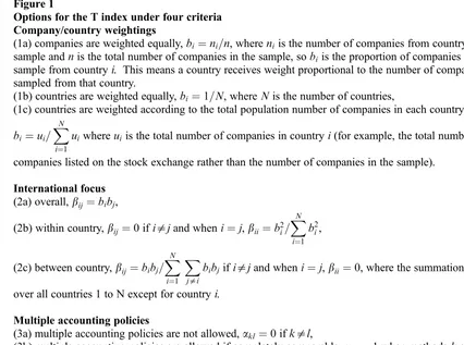
selected very generally to suit the particular data and research questions under analysis, in practice they can be determined by selecting from some intuitive options under four criteria. The four criteria and their respective options, summarised in Figure 1, are discussed in detail in Taplin (2004) and Taplin (2006). Thefirst two criteria define the bijand the last two criteria define theakl.
Thus theTindex represents an extremelyflexible framework containing an uncountable number of specific indices, including many simpler indices. The H index equals the T index under options 1a2a3a4a but is usually applied to a single country. Figure 1
Options for the T index under four criteria Company/country weightings
(1a) companies are weighted equally,bi¼ni=n, whereniis the number of companies from countryiin the
sample andnis the total number of companies in the sample, sobiis the proportion of companies in the
sample from countryi. This means a country receives weight proportional to the number of companies
sampled from that country.
(1b) countries are weighted equally,bi¼1=N, whereNis the number of countries,
(1c) countries are weighted according to the total population number of companies in each country,
bi¼ui=
XN
i¼1
uiwhereuiis the total number of companies in countryi(for example, the total number of
companies listed on the stock exchange rather than the number of companies in the sample).
International focus (2a) overall,bij¼bibj,
(2b) within country,bij¼0ifi=jand wheni¼j,bii ¼b
2
i=
XN
i¼1 b2i,
(2c) between country,bij¼bibj=
XN
i¼1
X
j=i
bibjifi=jand wheni¼j,bii ¼0, where the summation forjis
over all countries 1 to N except for countryi.
Multiple accounting policies
(3a) multiple accounting policies are not allowed,akl¼0ifk=l,
(3b) multiple accounting policies are allowed if completely comparable,akl¼1when methodskandlare
completely comparable andakl¼0when they are completely incomparable,
(3c) multiple accounting policies are allowable with fractional comparability,akltakes a value on the
continuum from 0 (completely incomparable) to 1 (completely comparable).
Non-disclosure
Here it is assumed non-disclosure is the last accounting methodM.
(4a) not applicable, companies who do not disclose a method are removed from the sample,
(4b) comparable to everything,akM¼aMl¼aMM¼1for all accounting methodskandl,
(4c) comparable to nothing,akM¼aMl¼aMM¼0for all accounting methodskandl,
(4d) comparable to the standard (or default) methods,aks¼akM,asl¼aMlfor allkandl.
The H and T indices employ sampling with replacement when selecting two companies for comparison while the C index employs sampling without replacement. Taplin (2004) provides rea-sons why sampling with replacement is preferable, but in practice both index values will be almost identical unless sample sizes are very small. Similarly, the within countryCindex gives almost identical values to the T index under options 1a2b3a4a. The between-country C index and T
index under options 1a2c3a4a give identical results since sampling with or without replacement are equivalent when only one company is selected from each country. For two countries, theIindex equals the between-country C index (Morris & Parker, 1998) andTindex (options 1a2c3a4a) but for more than two countries theIindex is not a special case of the T index. See Taplin (2004) for a review of undesirable properties of theIindex with more than two countries.
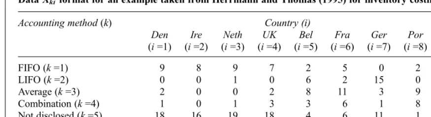
This paper takes illustrative data and examples from Herrmann and Thomas (1995) to illustrate the methods in this paper. Their study is well known as a comparative evaluation, has moderate sample sizes, the data is already published so results in this paper can be verified, their examples include issues such as non-disclosure and combination methods, and the effect of different methods on conclusions can be seen more clearly because the same data has been examined in the literature using different methods.
Table 1 illustrates the format of the data required for the T index using an example for inventory costing from Herrmann and Thomas (1995). In this example there are N¼8 countries and M¼5 accounting methods for inventory costing (non-disclosure of the treatment of inventory costing is thefifth‘method’). Countries are referred to by the index i (i=1 to N) and accounting methods are referred to by the index k (k=1 to M). The data consists of the number of companies in country i
using method k, denoted Xki and displayed in
Table 1. Sample sizes for each country, denotedni
are also provided.
We illustrate the calculation of theTindex under options 1a2a3a4a. This means that companies are weighted equally, all companies regardless of country are compared (overall international focus), multiple accounting policies do not exist and companies not disclosing a method are removed (leaving only M¼4 methods). We use these options for illustrative purposes only and do not suggest they are the most appropriate options for this data. In this case Equation (1) is a summation of 4646868¼1;024terms, although at least 75% (or 126868¼768) of these terms equal zero because 12 of the 16akl equal zero. Nevertheless,
the T index generally contains a large number of terms and a systematic approach is required. This is provided by the observation that Equation (1) can be written as
T¼X
N i¼1
XN
j¼1
XM
k¼1
XM
l¼1
aklbijpkiplj¼
XN
i¼1
XN
j¼1 bijTij
where
Tij¼
XM
k¼1
XM
l¼1 aklpkiplj
is the two-country index quantifying the level of harmony between countryiand countryjandbijare the weights assigned to theTijwhen computing the
weighted average. With options 3a and 4a the akl
equal zero whenk=land theakkequal one, soTii
simplifies to the H index for countryiandTij(i=j)
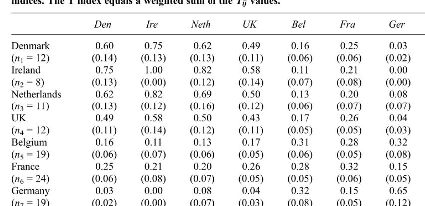
simplifies to theIindex for countriesiandj. These values are provided in Table 2 with the calculation ofT11andT31illustrated beneath the table.
The value of T¼X
N
i¼1
XN
j¼1
bijTij is a weighted
average of theTijvalues in Table 2. The weights in
this average under options 1a and 2a are bij¼bibj ¼ninj=n2 where ni is the sample size
Table 1
DataXkiformat for an example taken from Herrmann and Thomas (1995) for inventory costing
Accounting method(k) Country (i) Total
Den
(i=1)
Ire
(i=2)
Neth
(i=3)
UK
(i=4)
Bel
(i=5)
Fra
(i=6)
Ger
(i=7)
Por
(i=8)
FIFO (k=1) 9 8 9 7 2 5 0 2 42
LIFO (k=2) 0 0 1 0 6 2 15 0 24
Average (k=3) 2 0 0 2 8 11 3 9 35
Combination (k=4) 1 0 1 3 3 6 1 8 23
Not disclosed (k=5) 18 16 19 18 4 6 11 1 93
Sample size (ni) 30 24 30 30 23 30 30 20 217
for countryi(see column 1 of Table 2) andn¼124 is the total sample size. Thefirst three terms of this sum are provided beneath Table 2. The resulting value ofT¼0:27(options 1a2a3a4a) results from the large spread of companies using different methods and implies there is only a 27% chance of two randomly selected companies having accounts that are comparable. Under options 1b2a3a4a the weights bij all equal 1/64 and
T¼0:31 is a simple average of the 64 Tij in Table 2.
If we consider the accounts of non-disclosing companies to be not comparable with accounts of all other companies (option 4c instead of 4a) then
T¼0:087. In this caseM¼5since non-disclosure is included as an accounting method and the high level of non-disclosure results in a lower value of theTindex. Note theTijwill be lower than those in
Table 2 due to the comparability of non-disclosure and thebij will differ since the sample sizesni(and hencen) will be higher.
Many international accounting studies prefer to examine the comparability of companies between
different countries (option 2c), a property of theI
index and between-countryCindex. If, as with theI
index, we give each country equal weight (option 1b), bij equals 1/56 when i=j and bii¼0. Then
T¼0:27(option 1b2c3a4a) is a simple average of the off-diagonal entries in Table 2. If companies are weighted equally (option 1a2c3a4a) we obtain the between-countryCindex value ofT¼0:24. If non-disclosing companies are considered non-compar-able to all other companies (option 4c) these values for theTindex are 0.079 and 0.076 respectively.
The choice of akl and bij in any application
requires careful consideration and justification. These examples are for illustration only and we do not claim any of the above choices are optimal. Indeed, calculating and reporting values of the T
index under different assumptions or options, as above, is recommended. The flexibility of the T
index provides a unified framework for comparison of indices, encourages careful thought of the appropriate index for a particular problem, enhances investigations into the sensitivity of conclusions to the choice of index, and opens up Table 2
Tij under options 3a4a (with standard errors in parentheses). Diagonal entriesTiiequal H indices for
country i and off-diagonal entriesTij (i=j) equal two-country I (or equivalently between-country C)
indices. The T index equals a weighted sum of theTijvalues.
Den Ire Neth UK Bel Fra Ger Por
Denmark
(n1= 12)
(0.60 (0.14) (0.75 (0.13) (0.62 (0.13) (0.49 (0.11) (0.16 (0.06) (0.25 (0.06) (0.03 (0.02) (0.19 (0.07) Ireland
(n2= 8)
(0.75 (0.13) (1.00 (0.00) (0.82 (0.12) (0.58 (0.14) (0.11 (0.07) (0.21 (0.08) (0.00 (0.00) (0.11 (0.07) Netherlands
(n3= 11)
(0.62 (0.13) (0.82 (0.12) (0.69 (0.16) (0.50 (0.12) (0.13 (0.06) (0.20 (0.07) (0.08 (0.07) (0.12 (0.06) UK
(n4= 12)
(0.49 (0.11) (0.58 (0.14) (0.50 (0.12) (0.43 (0.11) (0.17 (0.05) (0.26 (0.05) (0.04 (0.03) (0.25 (0.06) Belgium
(n5= 19)
(0.16 (0.06) (0.11 (0.07) (0.13 (0.06) (0.17 (0.05) (0.31 (0.06) (0.28 (0.05) (0.32 (0.08) (0.28 (0.06) France
(n6= 24)
(0.25 (0.06) (0.21 (0.08) (0.20 (0.07) (0.26 (0.05) (0.28 (0.05) (0.32 (0.06) (0.15 (0.05) (0.34 (0.05) Germany
(n7= 19)
(0.03 (0.02) (0.00 (0.00) (0.08 (0.07) (0.04 (0.03) (0.32 (0.08) (0.15 (0.05) (0.65 (0.12) (0.10 (0.05) Portugal
(n8= 19)
(0.19 (0.07) (0.11 (0.07) (0.12 (0.06) (0.25 (0.06) (0.28 (0.06) (0.34 (0.05) (0.10 (0.05) (0.41 (0.06) Examples:
From the number of companies using each method in each country (see Table 1):
T11¼ ð9=12Þ 2
þ ð0=12Þ2þ ð2=12Þ2þ ð1=12Þ2¼0:60
T13¼ ð9=12Þð9=11Þ þ ð0=12Þð1=11Þ þ ð2=12Þð0=11Þ þ ð1=12Þð1=11Þ ¼0:62
The T index is given by the weighted average ofT¼X
N i¼1
XN
j¼1
bijTijwherebijare defined by options 1 and
2. Under options 1a2a (companies weighted equally and overall international focus),bij¼ninj=n2for all
values ofiandjsoTequals the sum of 64 terms as follows (first three terms shown only):
T¼ ð12612=1242
Þ60:60þ ð8612=1242
Þ60:75þ ð12611=1242
Þ60:62þ:::¼0:27
possibilities of new indices tailor made for a specific problem.
3. Statistical inference for the T index
The T index given by Equation (1) is typically calculated using sample data consisting of propor-tionspkiequal to the proportion of companies in thesample of companies from country i that use accounting methodk. When considering statistical inference for the T index it is important to distinguish between this index based on a sample of companies and the corresponding index based on the population of all companies from these coun-tries. We refer to the latter as the populationTindex, denotedTp. It is given by
Tp¼
XN
i¼1
XN
j¼1
XM
k¼1
XM
l¼1
aklbijpkiplj ð2Þ
where
pki equals the proportion of companies using
accounting method k out of all the com-panies in the population of comcom-panies from countryi, and
plj equals the corresponding proportion for
methodland countryj.
In practice, it is not possible to include all companies in all countries in our sample and hence the sample T index is only an estimate of the population index Tp. Here we consider the
statistical properties of the sampleT index and in particular how accurate it is as an estimate of the corresponding index in the population.
3.1. The bias of the T index
The bias of an estimate is defined as the difference between the expected value of the sample estimate and the quantity being estimated, and hence equals zero only if the mean of the sampling distribution equals the quantity being estimated.
The bias of the T index is derived in the Appendix to equal the summation in Equation (3) (boxed below).
Although this bias appears a complicated expres-sion that can be positive, negative or zero, there are a few important characteristics that we now discuss. The bias ofTwill equal zero if thebiiall equal zero, and in particular for anyTindex under option (2c) utilising a between-country focus. This is an
important special case because international studies often focus on comparisons between countries. With this international focus, we now know that the value of the T index calculated from a random sample will, on average, equal the value of the
T index calculated from the entire population. In particular, this result proves the between country C index of Archer et al. (1995) and the two-country I index of van der Tas (1988) are both unbiased.
Further insights into the bias of theTindex can be obtained by writing Equation (3) as
biasðTÞ ¼X
N i¼1
bii ni
Di Ti
ð Þ: ð4Þ
where
Di¼
XM
k¼1 akkpki
and
Ti¼
XM
k¼1
XM
l¼1
aklpkipli:
In many applications of theTindex an accounting method will be considered completely comparable with itself (so theakkwill all equal 1) except where
one accounting method represents non-disclosure in which case thisakk may be zero. In this case, Di
equals the proportion of companies in the popula-tion of country i that disclose their accounting method. When all companies disclose their account-ing method, Di will typically equal 1. Although
uncommon in the past literature (Astami et al. (2006) is an exception)akkcan be between 0 and 1
due to partial disclosure, as discussed in the Introduction.
TheTimeasure national comparability, the level
of comparability for companies from countryi, and are based on the population of all companies from countryi. For example, ifakl equals 1 whenk¼l
and equals 0 whenk=l, thenTiequals the value of
the Herfindahl H index applied to all companies from countryi.
From Equation (4) several observations can be made concerning the bias of theTindex. First, the bias is rarely negative because it is unlikelyTiwill
be greater thanDifor any country. Ifaklakkfor
all values ofkandl, which is plausible in practice because it states that an accounting methodkis at biasðTÞ ¼X
N
i¼1
X
M
k¼1
akkbiipki=ni
X
N
i¼1
X
M
k¼1
X
M
l¼1
aklbiipkipli=ni: ð3Þ
least as comparable with itself than with any other accounting method, then TiDi and so from
Equation (4) the bias is not negative.2
Second, sinceDiandTiare both between 0 and
1, their difference must be at most 1 in magnitude. Hence the magnitude of the bias can not be greater
than X
N
i¼1
bii=ni. In practice this is a useful upper
bound because it can be calculated prior to data collection since it only depends on the sample size and the international focus to be used for the
Tindex. This implies that the bias will be negligible in large sample sizes.
In summary, the bias will be zero for a between country focus and small if the within country
weighting given byX
N
i¼1
biiis small or if the sample
sizes for the countries are all large. For most plausible indices and practical data, the bias will be zero or negligible.
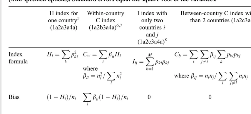
3.2. The standard error for the T index
Formulae to calculate the standard error of the
T index are provided in the Appendix. Since the formulae are complicated and not particularly intuitive they are presented in a format suitable for implementation rather than to provide intuitive insights. Examples in the following sections will provide insights into the magnitude of the standard error in different situations.
Instead, Table 3 provides formulae for the variance of the special cases of the T index corresponding to simpleH,I, and between-country and within-countryCindices. The overallCindex gives values slightly different to the Hindex and
T index (option 1a2a3a4a) due to differences between sampling with or without replacement, but these differences are negligible unless sample sizes are very small. Similarly, the within-country
C index will give slightly different values to the
T index under options 1a2b3a4a unless sample sizes are very small. The other indices in Table 3 give exactly the same value as theTindex with the options specified.
We illustrate the use of the formula for the two-country I index between the UK and Belgium (I = 0.17, SE = 0.05, see Table 2). From Table 1, and after ignoring companies not disclosing their accounting method, we have for the UK (i¼4),
pk4 equal to 7/12, 0, 2/12, and 3/12 (n4¼12) for
accounting methodsk= 1 to 4 respectively, while
for Belgium (i¼5) the corresponding proportions
pk5 equal 2/19, 6/19, 8/19, and 3/19 (n5¼19).
Using these as estimates for thepki we obtain the values foryklð34Þprovided in Table 4, and summing
these values gives a variance of 0.00248. The standard error of 0.05 reported in Table 2 is the square-root of this variance.
The formula for the variance of the between-country C index with more than two countries requires a table ofyklðijÞ, as well as a corresponding table offklðijÞ, for each pair of countriesiandj. The fklðijÞ terms account for correlations between two-countryIindices that have a country in common, such as theIindex between countries 1 and 2 and theIindex between countries 1 and 3.
The formulae for the bias and variance of the within-country C index and between-country
Cindex in Table 3 are valid for any choice of thebii
and bij respectively. The values bii¼n2i=X
i
n2i
and bij¼ninj=
X
i
X
j=i
ninj are specified in the
formulae for the indices only because these corres-pond to option 1a (companies weighted equally) used byCindices. International studies that prefer, for example, to weight countries equally (option 1b) can use the formulae for bias and variance in Table 3 by specifying bii ¼1=N for the within index and bij¼1=ðNðN 1ÞÞfor the between-country index.
4. The nine measurement practices of
Herrmann and Thomas (1995)
Herrmann and Thomas (1995) examined the level of comparability in Belgium, Denmark, France, Germany, Ireland, the Netherlands, Portugal and the UK using data from the 1992–1993 annual reports of 217 companies. They used a modification of the
Iindex by substituting values of 0.01 and 0.99 when the proportion of companies within a country using a particular method were 0 and 1 respectively. They argued this modification was necessary because‘the
Iindex is sensitive to zero proportions’and that this ‘potential sensitivity increases as the number of countries surveyed increases’ (Herrmann and Thomas, 1995: 256). Taplin (2004) discussed problems with the I index for more than two countries and with this ad hoc adjustment. Table 1 reproduces the data for the measurement practice of inventory costing. Data for all nine measurement practices is available in Herrmann and Thomas (1995).
Table 5 contains theIandTindex values for the data on the nine measurement practices in Herrmann and Thomas (1995). These T index
2A proof of this result is available from the author upon
request.
Table 3
The formulae, bias and variance of the simple H, I and C indices that are special cases of the T index (with specified options). Standard errors equal the square-root of the variances.
H index for
one country5
(1a2a3a4a)
Within-country C index
(1a2b3a4a)6,7
I index with only two
countriesi
andj
(1a2c3a4a)8
Between-country C index with more
than 2 countries (1a2c3a4a)5
Index formula
Hi¼
X
k
p2
ki Cw¼
X
i
biiHi
where bii¼n
2
i=
X
i
n2i
Iij¼
XM
k¼1 pkipkj
Cb¼
X
i
X
j=i
bijX
k
pkipkj
wherebij¼ninj=
X
i
X
j=i
ninj
Bias ð1 HiÞ=ni X
i
biið1 HiÞ=ni 0 0
Variance s2
Hi
X
i
b2iis2
Hi
X
k
X
l
yklðijÞ 2
X
i
X
j=i
bijX
k
X
l
ðbijyklðijÞ fklðijÞÞ
k,lare dummy indicators for possible accounting methods and take values 1 toM
i,j,Jare dummy indicators for possible countries and take values 1 toN
X
i
is a summation over all possible values ofifrom 1 toN
X
j=i
is a summation over all possible values ofjfrom 1 toNexcepti
niis the number of sampled companies from countryi.
pkiis the proportion of companies from countryiusing method k.
s2
Hi¼ X
k
akðiÞþ
X
k
X
l=k
bklðiÞ 1 ðn 1Þ
X
k
p2
ki
!2 =n2
i is the variance of the H index for countryi.
akðiÞ¼ ðpkiþ7ðni 1Þp2kiþ6ðni 1Þðni 2Þp3kiþ ðni 1Þðni 2Þðni 3Þp4kiÞ=n
3
i
bklðiÞ¼ ððni 1Þðni 2Þðni 3Þp2kip
2
liþ ðni 1Þðni 2ÞpkipliðpkiþpliÞ þ ðni 1ÞpkipliÞ=n3i
yklðijÞ¼ ð1 ni njÞpkipkjpliplj=ðninjÞ whenk=l, and
ykkðijÞ¼ ðni 1Þp2kiþpki
ðnj 1Þp2kjþpkj
=ðninjÞ p2kip
2
kj
fklðijÞ¼pkipkj
X
J=i;j
ðpliplJbiJ=niþpljplJbjJ=njÞwhenk=l, and
fkkðijÞ¼pkipkjX
J=i;j
ðpkJðpki 1ÞbiJ=niþpkJðpkj 1ÞbjJ=njÞ
where the summations overJare for all possible values of from 1 toNexceptiandj.
5
TheHindex and overallCindex are slightly different due to differences between sampling with or without replacement, but these differences are negligible unless sample sizes are very small. We present results for a single country here since this is how theHandCindices are typically used. If a simple random sample from several countries is taken then these formulae should be used for the bias and variance of theTindex under options 1a2a3a4a. If a stratified random sample is taken, where simple random samples of a pre-specified size are independently taken from each country, the general formula for the bias and variance of theTindex should be used.
6
TheT(1a2b3a4a) and within-countryCindices are slightly different due to differences between sampling with or without replacement, but these differences are negligible unless sample sizes are very small.
7These formulae for the bias and variance of the within-countryCindex and the between-countryCindex hold for other
choices of weightingsbij. For example, if countries are weighted equally (option 1b) rather than companies weighted equally (1a) assumed by theCindices, thenbii¼1=Nfor the within index andbij¼1=ðNðN 1ÞÞfor the between-country index. The provided formulae for the bias and variance of these indices still hold with these weighting of companies/countries.
8
This equals the between-countryCindex since there are two countries.
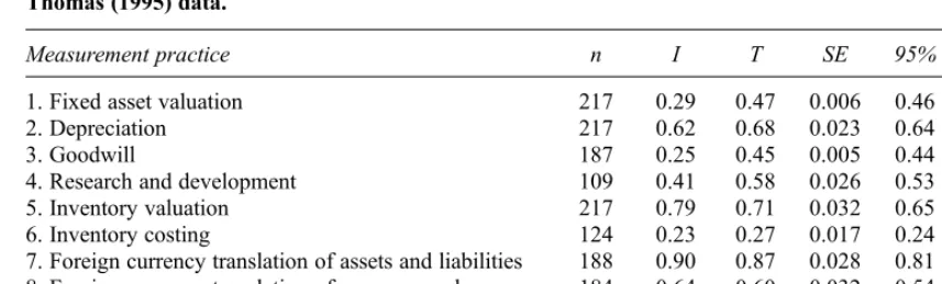
values were calculated using options 1b2c3a4a, so as with theIindex countries are weighted equally, comparisons are between different countries only, multiple accounting policies are not allowed and companies not disclosing their method are removed from the sample. Thus for measurement practice 6,
T¼0:27 equals the simple average of the off-diagonal entries in Table 2. Total sample sizes after removing non-disclosing companies and the stand-ard errors and 95% confidence intervals for the
Tindices are also presented.
From Table 5 we see that theIindex andTindex values are generally close, but differ by more than 0.10 for measurement practices 1, 3 and 4. The data for all of these contain zero proportions and hence are influenced by the arbitrary values of 0.01 and 0.99 substituted by Herrmann and Thomas (1995). For measurement practices 1 and 4 there are sufficient zero proportions in the data for the unmodified I index to equal 0. The I index in these circumstances is unstable, depending on whether the particular sample has proportions of zero or not and on the value of the arbitrary values of 0.01 and 0.99 substituted.
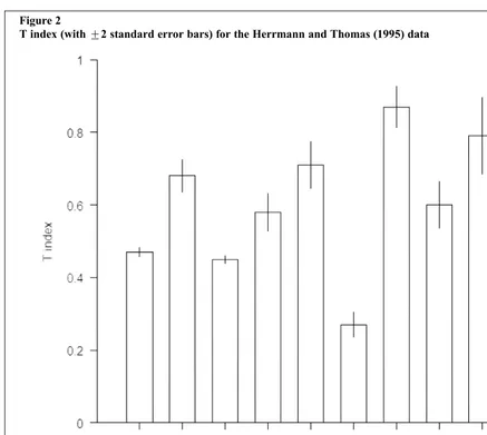
The standard errors for theTindex are generally small and indicate that the values of the T index calculated from this sample are accurate estimates. This is illustrated in Figure 2 where+2 standard error bars (representing 95% confidence intervals for the population index values) are presented graphically. This provides statistically significant evidence that the level of comparability for meas-urement practice 6 (Inventory costing) is lower than for any of the other eight practices since the 95% confidence intervals are far from overlapping. The evidence for measurement practice 7 (Foreign
currency translation of assets and liabilities) having the highest level of comparability is much weaker. Although in the sample data the index value of 0.87 for practice 7 is the highest, its confidence interval from 0.81 to 0.92 overlaps considerably with the confidence interval from 0.69 to 0.90 for practice 9 (Treatment of translation differences).
From Table 5 and Figure 2 we see that measure-ment practice 9 (Treatmeasure-ment of translation differ-ences) has a substantially larger standard error of 0.053 compared to the other practices. This is partially explained by the small sample size result-ing from the high level of non-disclosure for this practice. Table 5 reveals, however, other measure-ment practices such as 4 (Research and develop-ment) with both a smaller sample size and standard error.
The reason for the high standard error of 0.053 for practice 9 is because 15 of the 20 sampled companies from Portugal did not disclose their accounting method, resulting in an effective sample size of only 5 for Portugal. The higher standard error results from the fact that any comparisons between Portugal and another country cannot be made with statistical confidence. If companies had been weighted equally (option 1a under the
T index), then the standard error is reduced from 0.053 to 0.033, and similar to the standard errors for most of the other practices. Although comparisons with a Portugese company are prone to statistical inaccuracy, these comparisons are given little weight under option 1a because there is a small sample of companies from Portugal.
We do not suggest that the lower standard error under option 1a means that preference should be given to option 1a rather than option 1b when using Table 4
Values ofyklð34Þused to compute the standard error for the two-country I index (or between-country
C index) between the UK and Belgium for inventory costing in the Herrmann and Thomas (1995) data after removing non-disclosing companies.
k l
1 2 3 4
1 0.002012 0.000000 –0.000243 –0.000593
2 0.000000 0.000000 0.000000 0.000000
3 –0.000243 0.000000 0.002557 –0.000678
4 –0.000593 0.000000 –0.000678 0.000936
The sum of these 16 values gives the variance of theIindex equal to 0.00248. The standard error of 0.05
reported in Table 2 is the square-root of 0.00248.
Values ofyklð34Þin this table are calculated using the formula foryklðijÞbeneath Table 3, withi¼4(the UK)
andj¼5(Belgium) and the proportions estimated from the sample data in Table 1 as follows:pk4equal to
7/12, 0, 2/12, and 3/12ðn4¼12Þandpk5equal 2/19, 6/19, 8/19, and 3/19ðn5¼19Þfor k¼1to 4
respectively.
the T index. As described in Taplin (2004), the choice of options under the unified framework of the T index should be tailored to the specific research question being addressed. Rather, the example in the previous paragraph highlights the fact that it is more important to have higher sample sizes ineachcountry when equal weighting is given to each country than when companies are given equal weighting. The general principle is as follows: to obtain a more accurate value for theTindex (that is, a lower standard error), the sample size should be higher for countries that are given higher weight in theT index. For option 1b this suggests approxi-mately equal sample sizes in each country.
5. A comparison between fairness and
legalistic countries
Herrmann and Thomas (1995) also compared the level of comparability between the fairness coun-tries (Denmark, Ireland, the Netherlands and the UK) to the level of comparability between legalistic countries (Belgium, France, Germany and Portugal). They concluded on p. 264 that ‘The bicountry and four-country I indices reveal that fairness oriented countries are more harmonised than legalistic ones’. They made no attempt to examine the statistical significance of these differ-ences. Taplin (2003) reported this statistical com-parison, however only after using the H index instead of the I index. In Taplin’s (2004) unified framework of theTindex this required companies to be weighted equally (option 1a) instead of countries being weighted equally (option 1b) and an overall international perspective (option 2a) rather than a between-country perspective (option 2c).
Here we present the statistical comparison between the fairness and legalistic countries using options 1(b) and 2(c) of theTindex. For compari-son purposes with the results in Taplin (2003), we
begin by retaining the options 3(a) and 4(a) so, as with theHIndex in Taplin (2003), non-disclosing companies are removed prior to analysis.
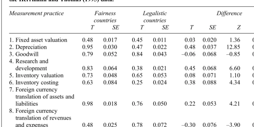
Table 6 contains the values for theTindex for the fairness and legalistic countries together with their standard errors. These are the four-country indices that are most comparable with theIindex used by Herrmann and Thomas (1995), but, avoids prob-lems associated with the various forms of the
I index for more than two countries. Table 6 also contains the difference inTindex values (Fairness countries T index minus legalistic countries
Tindex), the standard error of this difference, and standardised score Z and P-value when testing the null hypothesis of no difference inTindex values. Note that the standard error for the difference in
Tindex values equals the square-root of the sum of the squares of the two standard errors. For example, for the first measurement practice (Fixed asset valuation), the standard error for the difference in
Tindex values equals ffiffiffiffiffiffiffiffiffiffiffiffiffiffiffiffiffiffiffiffiffiffiffiffiffiffiffiffiffiffiffiffi0:0172
þ0:0112
p
¼0:020. As reported by Herrmann and Thomas (1995) the level of comparability is higher in the fairness countries for seven of the nine measurement practices. Measurement practice 3 (Goodwill) is one of the exceptions, but Table 6 shows that this difference of –0.06 is not statistically significant (P = 0.396). Thus this data is consistent with no difference in the level of comparability in fairness and legalistic countries, and indeed is consistent with either fairness or legalistic countries having the higher level of comparability.
The other exception is measurement practice 8 (Foreign currency translation of revenues and expenses). In this case, not only is the level of com-parability in the fairness countries smaller than the level in the legalistic countries (T= 0.48 compared to
T = 0.78), but this difference is highly significant statistically (P = 0.000). Although the overall trend Table 5
Total sample sizesnfor disclosing companies (summed over all countries), I indices and T (options 1b2c3a4a) indices (with standard errors and 95% confidence intervals) for the Herrmann and Thomas (1995) data.
Measurement practice n I T SE 95% CI
1. Fixed asset valuation 217 0.29 0.47 0.006 0.46 0.48
2. Depreciation 217 0.62 0.68 0.023 0.64 0.72
3. Goodwill 187 0.25 0.45 0.005 0.44 0.46
4. Research and development 109 0.41 0.58 0.026 0.53 0.63
5. Inventory valuation 217 0.79 0.71 0.032 0.65 0.77
6. Inventory costing 124 0.23 0.27 0.017 0.24 0.30
7. Foreign currency translation of assets and liabilities 188 0.90 0.87 0.028 0.81 0.92
8. Foreign currency translation of revenues and expenses 184 0.64 0.60 0.032 0.54 0.67
9. Treatment of translation differences 179 0.85 0.79 0.053 0.69 0.90
reported by Hermann and Thomas (1995) that fairness countries are more comparable is valid, this highly significant trend in the opposite direction for foreign currency translation of revenues and expenses may deserve further examination.
Furthermore, for two of the seven measurement practices where the level of comparability is higher in the fairness countries compared to the legalistic countries, the difference in the level of compar-ability is not statistically significant (P = 0.174 and P = 0.272 for practices 1 and 5). Thus there is statistically significant evidence that comparability is higher for fairness rather than legalistic countries in onlyfive of the nine measurement practices. The addition of this statistical rigour adds clarity to our interpretation of index values.
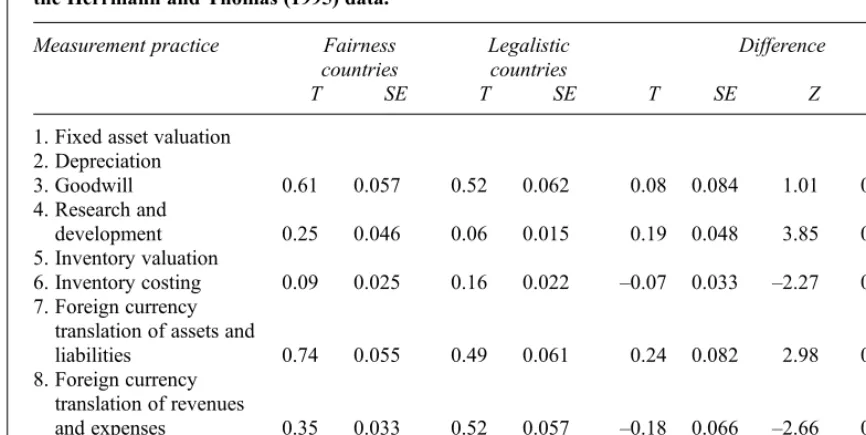
6. The effect of non-disclosure on the
standard error
Pierce and Weetman (2002) warned that interpret-ation of index values was problematic when the
non-disclosure level was high. Unlike the I index employed by Herrmann and Thomas (1995) and previousH andCindices, their adjusted C index does not remove all non-disclosing companies. Their analysis was, however, restricted by the lack of statistical inference techniques presented in this paper. We therefore repeat our comparison of the fairness and legalistic countries assuming com-panies not disclosing their accounting method are not comparable to all other companies.3This can be achieved by using option (4c) instead of (4a) under theT index framework. Results appear in Table 7 using the same format as in Table 6. For measure-ment practices 1, 2 and 5 all companies in the sample data disclosed their accounting method. In these cases results under option (4c) are identical to Figure 2
T index (with+2 standard error bars) for the Herrmann and Thomas (1995) data
3
For brevity we do not present results assuming non-disclosing companies are comparable with all other companies or, as Pierce and Weetman (2002) suggest, determining which companies are applicable and which are not-applicable non-disclosures.
results under option (4a) and so are not repeated in Table 7.
As expected, the change from option (4a) to (4c), whereby non-disclosing companies are considered non-comparable with all other companies, results in a lower level of comparability when non-disclosure exists. AllTindex values in Table 7 are smaller than the corresponding value in Table 6. Also as expected, these decreases are greatest where the level of non-disclosure is highest. For example, measurement practices 4 and 6 for the fairness countries have both the highest non-disclosure rate (with respectively 108 and 93 non-disclosing companies out of 217) and the highest reduction inTindex values, from 0.83 and 0.63 (Table 6) to 0.25 and 0.09 (Table 7) respectively.
Smaller sample sizes are typically associated with larger standard errors. However, removing non-disclosing companies does not necessarily increase standard errors. Exactly half of the 12 standard errors forTindices in Table 7 (with non-disclosing companies included) are smaller than the corresponding standard errors in Table 6 (where non-disclosing companies are removed). For meas-urement practice 7 in the fairness countries, the standard error triples from 0.018 to 0.055 when non-disclosing companies are included. This is because the very high value of 0.98 for theTindex under option (4a) is close to the boundary of 1 and this constrains the size of its standard error. This is
discussed in Section 8 where we consider the shape of the sampling distribution of theTindex.
The treatment of non-disclosure can have a large effect on the comparison between the level of comparability within the fairness and legalistic countries. Tables 3 and 4 both indicate a signifi -cant difference in the level of comparability within fairness and legalistic countries for measurement practice 6 (P = 0.000 and P = 0.023 respectively). However, the sign of the difference is not the same: under option (4a) where non-disclosing companies are removed the fairness countries have the higher level of comparability but under option (4c) where non-disclosing companies are con-sidered non-comparable the legalistic countries have the higher level of comparability. In this case conclusions concerning which group of countries is more comparable depends significantly on the treatment of non-disclosure. In contrast, we note that while the difference in T index values in Tables 3 and 4 for measurement practice 3 have different signs, neither is significantly different to zero (P = 0.396 and P = 0.314 respectively). No ambiguity in conclusions arises for measurement practice 3 because there is insignificant evidence of any difference in the level of comparability for fairness compared to legalistic countries. Although p-values in Tables 3 and 4 for the other measure-ment practices do change, conclusions remain the same if they are based on the conventional signifi -Table 6
A statistical comparison of the T indices (option 1b2c3a4a) for the fairness and legalistic counties and the Herrmann and Thomas (1995) data.
Measurement practice Fairness countries
Legalistic countries
Difference
T SE T SE T SE Z P-value
1. Fixed asset valuation 0.48 0.017 0.45 0.011 0.03 0.020 1.36 0.174
2. Depreciation 0.95 0.030 0.47 0.022 0.48 0.037 12.85 0.000***
3. Goodwill 0.79 0.052 0.84 0.043 –0.06 0.068 –0.85 0.396
4. Research and
development 0.83 0.064 0.38 0.021 0.45 0.068 6.60 0.000***
5. Inventory valuation 0.73 0.048 0.65 0.053 0.08 0.071 1.10 0.272
6. Inventory costing 0.63 0.084 0.25 0.024 0.38 0.088 4.34 0.000***
7. Foreign currency translation of assets and
liabilities 0.98 0.018 0.76 0.050 0.22 0.053 4.21 0.000***
8. Foreign currency translation of revenues
and expenses 0.48 0.025 0.78 0.072 –0.30 0.076 –3.90 0.000***
9. Treatment of translation
differences 0.92 0.042 0.67 0.091 0.25 0.100 2.48 0.013*
*, ** and *** denotes statistical significance at the 0.05, 0.01 and 0.001 level respectively (two-tailed tests).
cance level of 5% and on the direction of the difference.
7. The special case of the two-country I index
As shown in Section 2 the two-countryIindex, or the equivalent between country C index for two countries, is important because it is a basic ingre-dient in the calculation of the T index. We investigate the statistical properties of this special case of theT index in this section because some studies will compare only two countries. This will also provide additional insights into the accuracy with which T index values can be estimated (and later in Section 8 the extent to which the sampling distribution deviates from normality) when sample sizes are small. Table 2 contains the standard errors (in parentheses) for each of the two-countryI indices for measurement practice 6 (Inventory costing) and Section 3.2 illustrates the calculation of these standard errors.
Fairness countries (listed first in Table 2) have higher values for the two-countryIindex (ranging from 0.49 to 0.82) than legalistic countries (ranging from 0.10 to 0.34) or between a fairness and legalistic country (ranging from 0.00 to 0.26). They also have higher standard errors (ranging from 0.11 to 0.14 compared to 0.05 to 0.08 and 0.00 to 0.08 respectively), reflecting the lower level of accuracy with which we have estimated the degree of comparability between fairness countries. This is
largely due to the smaller sample sizes for the fairness countries, which result in part from the higher level of non-disclosure in these countries. The lowest level of comparability between two fairness countries is 0.49 (SE = 0.11) between Denmark and the UK. This is not significantly higher than the comparability between some pairs of legalistic countries. For example, the level of comparability between France and Portugal is 0.34 (SE = 0.05).
Finally, we note for measurement practice 6 in Table 5 the standard error of 0.017 is considerably lower than 0.071, the mean of the off-diagonal standard errors in Table 2. Recall (see Section 2) the corresponding value ofT¼0:27in Table 5 is the mean of the off-diagonal index values in Table 2. The lower standard error in Table 5 is a direct result of the Tindex using data from all eight countries while each of the indices in Table 2 uses data from only two countries: indices based on larger samples are expected to have similar values, on average, but with smaller standard errors.
This smaller standard error for an index based on several countries compared to the standard error for an index based on two countries has implications when designing studies. The recommendation in Taplin (2004) to examine the two-countryIindices whenever calculating a T index with several countries is still relevant, however if research questions relate to comparisons between pairs of Table 7
A statistical comparison of the T indices (option 1b2c3a4c) for the fairness and legalistic counties and the Herrmann and Thomas (1995) data.
Measurement practice Fairness countries
Legalistic countries
Difference
T SE T SE T SE Z P-value
1. Fixed asset valuation 2. Depreciation
3. Goodwill 0.61 0.057 0.52 0.062 0.08 0.084 1.01 0.314
4. Research and
development 0.25 0.046 0.06 0.015 0.19 0.048 3.85 0.000***
5. Inventory valuation
6. Inventory costing 0.09 0.025 0.16 0.022 –0.07 0.033 –2.27 0.023*
7. Foreign currency translation of assets and
liabilities 0.74 0.055 0.49 0.061 0.24 0.082 2.98 0.003**
8. Foreign currency translation of revenues
and expenses 0.35 0.033 0.52 0.057 –0.18 0.066 –2.66 0.008**
9. Treatment of translation
differences 0.65 0.057 0.40 0.049 0.25 0.075 3.31 0.001***
*, ** and *** denotes statistical significance at the 0.05, 0.01 and 0.001 level respectively (two-tailed tests).
countries as well as between all countries then larger sample sizes may be required. We discuss the issue of required samples sizes in Section 9.
8. The sampling distribution for the T index
This paper has presented formulae for the standard error of the T index and applied them to several examples. The formulae are exact under independ-ent random sampling of companies from countries without any additional assumptions, but the confi -dence intervals and p-values derived from these standard errors also assume that the sampling distribution of theTindex is normal. For example, 95% confidence intervals were constructed with the estimated T index plus or minus 1.96 standard errors and Z scores were converted into p-values using standard normal tables. In practice, normality is often a good approximation for this sampling distribution, especially in large sample sizesni orwhen there is a large number of countries, due to Central Limit Theorem results. First, when the sample sizeniis large the correspondingpkifor that
country will be approximately normally distributed. Second, since theTindex is a weighted average of random variables, when this average is over a larger number of terms the sampling distribution is likely to be closer to normal.
Central Limit Theorem results, however, provide limits as sample sizes tend to infinity and are therefore of theoretical interest. Instead, we provide some examples of the sampling distribution for the
Tindex so the accuracy of the normal distribution can be evaluated in more realistic finite samples. We do so by providing histograms of one million
T index values generated from one million simu-lated samples from known populations. Not only do these simulations allow a comparison with the normal distribution, the interval from the 0.025 percentile to the 0.975 percentile of these distribu-tions provides an exact 95% interval to compare with the approximate plus or minus 1.96 standard error approximation based on normality. Since the approximation is extremely accurate in most examples covered in this paper, we concentrate on cases where the approximation is weakest. Although two decimal places are generally suffi -cient when using a confidence interval to assess the accuracy of an estimate, in this section we quote intervals to three decimal places to allow closer scrutiny of the accuracy of this normality approxi-mation.
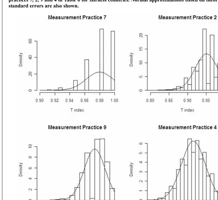
A value ofT¼0:98(and standard error of 0.018) was reported in Table 6 for fairness countries and measurement practice 7. In this case, it is clear that the sampling distribution can not be normal because
the upper bound for a legitimateTindex value is 1, only just over one standard error from the estimate. Furthermore, a 95% confidence interval calculated with the plus or minus 1.96 standard error rule will be non-sensible in this case since it will include values beyond the theoretical boundaries of 0 and 1. Of the 54T index values presented in Tables 2, 3 and 4 there are three occasions where these approximate confidence intervals for the T index using the plus or minus 1.96 standard errors rule result in intervals extending past either 0 or 1. These are for fairness countries with measurement prac-tices 7, 2, and 9 (whereTindex values are 1.0, 1.8 and 1.9 standard errors from the nearest boundary). We also include measurement practice 4 for the fairness countries since its T index value is 2.6 standard errors from the boundary of 1. No other
Tindex is within 3 standard errors of a boundary of 0 or 1.
Figure 3 presents the estimated sampling distri-bution from the results of simulating one million samples from each of these populations. That is, these histograms describe the probability of obtain-ing different values for the T index when randomly sampling companies. Each distribution has the normal distribution superimposed that uses the theoretical standard error given in Section 3.2. Note that in each of these cases the bias is zero since the indices use a between country international per-spective (option 2c).
Measurement practice 7 (top left of Figure 3) shows a sampling distribution that is clearly not normal, as expected since the mean of the distribu-tion is only 1.0 standard errors from the boundary of 1. It is highly skewed and discrete in nature with only a few index values possible. Indeed, this sampling distribution only contains the possible values of 1 and multiples of 0.018 less than 1 (1, 0.982, 0.964, ) corresponding to none, one, two, sampled companies using the current/histor-ical method rather than the historcurrent/histor-ical method. Only one of the 99 companies from the fairness countries in this data used the current/historical method.
Despite this clear non-normality for measure-ment practice 7, the approximate 95% interval calculated using the plus or minus 1.96 standard errors rule is accurate. In this case, the approxima-tion gives the interval from 0.948 to 1.017. The 95% interval calculated using the 0.025 and 0.975 percentiles from the million simulations yields an interval from 0.946 to 1.
Measurement practices 2, 9 and 4 show progres-sively lower degrees of non-normality with the means of the sampling distributions being 1.8, 1.9 and 2.6 standard errors from a boundary. Their
approximate intervals are 0.889 to 1.005, 0.839 to 1.004 and 0.705 to 0.957 respectively. The intervals based on the percentiles are 0.882 to 1, 0.823 to 1 and 0.694 to 0.962 respectively. In each case the approximate intervals are accurate within 0.02 and usually accurate within 0.01. Hence the approxi-mations are extremely accurate, especially com-pared to the inaccuracy in the estimated T index values summarised by the length of the intervals.
All of the other 50 T index values presented in Tables 2, 3 and 4 are more than three standard errors from the boundaries of 0 and 1 and the approximate 95% confidence intervals formed by taking the estimatedTindex value plus or minus 1.96 standard errors are very accurate. Practical experience sug-gests that this approximation is extremely accurate when theTindex is more than three standard errors
from both boundaries of 0 and 1. Furthermore, it is likely to be accurate to within 0.01 if theTindex is more than two standard errors from both boundaries of 0 and 1, and often accurate even when this is not the case.
Hence we conclude that statistical inference performed as if the sampling distribution of the
Tindex is normal is likely to be sufficiently accurate for most purposes unless possibly when the estimated index value is within two standard errors of a boundary. This is likely to occur when either there is a very high or low level of comparability resulting in aTindex value that is close to either 0 or 1, or the standard error is very high reflecting an inaccurate estimate of the populationTpindex value
due to samples sizes that are too small.
Normality is less likely to be a valid approxima-Figure 3
Sampling distributions based on 1,000,000 samples for the T index corresponding to measurement practices 7, 2, 9 and 4 in Table 6 for fairness countries. Normal approximations based on theoretical standard errors are also shown.
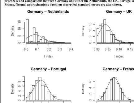
tion for the two-country I indices for Inventory costing in Section 7. This is because theseTindices are calculated from a sum involving fewer terms and the standard errors tend to be higher. Figure 4 displays the sampling distribution for some of the two-countryIindices in Table 2. The Netherlands, the UK, Portugal and France were chosen for illustration purposes because the index values between these countries and Germany are close to a boundary of 0 or 1 (respectively 1.1, 1.5, 2.1 and 2.8 standard errors away).
From Figure 4 it is apparent that normality is a poor approximation when the value for theTindex is close to a boundary of 0 or 1 (compared to the size of the standard error). For the Netherlands and the UK, approximate 95% confidence intervals using the value of theTindex plus or minus 1.96 standard errors result in intervals including negative values (–0.059 to 0.212 and–0.013 to 0.092 respectively). The intervals from the 0.025 and 0.975 percentiles of the simulated distribution are 0.000 to 0.244 and 0.000 to 0.105 respectively. For Portugal, the sampling distribution is slightly skewed but close
to normal. The approximate 95% confidence inter-val of 0.005 to 0.189 is close to the interinter-val of 0.019 to 0.199 from the simulation. In this case the value for theIindex is just over two standard errors from the closest boundary. Finally, for the I index comparing Germany and France theIindex is 2.8 standard errors from the boundary and the sampling distribution is very close to normal. The approxim-ate 95% confidence interval 0.046 to 0.256 and interval of 0.048 to 0.259 from the simulation are very close.
Once again these approximations are accurate, especially if the presence of intervals extending beyond the boundaries of 0 and 1 are ignored and the accuracy of the approximate intervals are compared to the length of the intervals.
9. Sample size determination
The formula for the standard error of the T index can be used to determine the necessary sample sizes for each country in order to achieve a given level of precision for the T index. We now illustrate this procedure for a simple example.
Figure 4
Sampling distributions based on 1,000,000 samples for the I index corresponding to measurement practice 6 and comparisons between Germany and either the Netherlands, the UK, Portugal or France. Normal approximations based on theoretical standard errors are also shown.
Germany–Netherlands
Germany–Portugal
Germany–UK
Germany–France
Suppose we are planning a study involving four countries and we anticipate three accounting methods, labeled A, B and ND for non-disclosure. First we select theTindex we desire for our study. Companies do not provide enough information in their accounts to enable comparability with both a company using method A and another company using method B so multiple accounting policies are not possible (option 3a). Furthermore, we consider non-disclosure to be not comparable (option 4c). We wish to make between-country compariso