Classroom Behavior
Carmit Segal
a b s t r a c t
This paper investigates the determinants and malleability of noncognitive skills. Using data on boys from the National Education Longitudinal Survey, I focus on youth behavior in the classroom as a measure of noncognitive skills. I find that student behavior during adolescence is persistent. The variation in behavior can be attributed to unobserved individual heterogeneity. Family and school characteristics, as well as the incentives for good behavior provided at home and in school, are important determinants of behavior. Neither the cross-sectional variation in behavior nor the variation over time in behavior can, however, be attributed to these covariates.
I. Introduction
Several recent papers have demonstrated the importance of noncog-nitive skills to labor market success (Bowles, Gintis, and Osborne 2001; Cawley, Heckman, and Vytlacil 2001; Jacob 2002; Persico, Postlewaite, and Silverman 2004; Borghans, ter Weel, and Weinberg 2005; Segal 2005, Fortin 2008; Heckman, Stixrud, and Urzua 2006). In labor market settings it seems important to take into account the assignment of workers to jobs to explain why some noncognitive skills are in higher demand than others (Borghans, ter Weel, and Weinberg 2008; Krueger and Schkade 2008). Among the noncognitive skills that have been investigated to this date are interpersonal interactions, behavior in the classroom, and various personality traits like aggression, externality, self-esteem, and friendliness. Unfortunately, one cannot conclude from the above-mentioned studies that it is possible to design pol-icies that would directly affect noncognitive skills. In particular, if noncognitive skills were predetermined by family characteristics, like parental income and
The author would like to thank her advisors, Ed Lazear, Muriel Niederle, and Ed Vytlacil for their encouragement, useful suggestions, and numerous conversations; members of the Stanford Labor group for useful discussions; seminar participants at Cornell University and at the University of Florida; three anonymous referees, Liran Einav, Florian Englmaier, Avner Greif, Susanna Loeb, Amalia Miller, John Pencavel, Luigi Pistaferri, Ravi Singh, Frank Wolak, and Nese Yildiz for helpful comments. Special thanks to Ilona Berkovits for access to, and assistance with the data. The author is grateful to Harvard Business School for generous support and hospitality and thanks the support of the Barcelona Economics Program of CREA. The data used in this article can be obtained beginning May 2009 through April 2012 from Carmit Segal, Department of Economics and Business, Universitat Pompeu Fabra, Ramon Trias Fargas 25-27, Barcelona, Spain 08005Æcarmit.segal@upf.eduæ.
½Submitted May 2006; accepted December 2006
ISSN 022-166X E-ISSN 1548-8004Ó2008 by the Board of Regents of the University of Wisconsin System
education, there would be little scope for policies directly targeting noncognitive skills. Moreover, before designing policies targeting noncognitive skills, it is impor-tant to understand to what degree these skills can be changed. The recent literature evaluating social policies suggests encouraging indirect evidence. Cunha and Heckman (2008) show that there are distinct sensitive periods for the development of cognitive and noncognitive skills and that investment is complementary. Heckman (2000) and Carneiro and Heckman (2003) suggest that programs like early intervention pro-grams or mentoring and teenage motivation propro-grams may be successful because they affect noncognitive skills. This paper takes another step in assessing whether policies that target noncognitive skills could be effective by investigating their mal-leability and origins. The analysis focuses on one measure of noncognitive skills— adolescent behavior in the classroom—as measured by teacher evaluations of male participants in the National Educational Longitudinal Survey (NELS) data set. I explore its persistence, as well as how it relates to family and school characteristics. Substantial research effort has been invested in understanding youth delinquent and antisocial behavior (for an excellent summary of the research on antisocial be-havior in children and youth, see Dodge 2006), and on trying to prevent it (see, for example, Gerstenblith et al. 2005 for a summary of the evidence on the effects of after school programs). In this paper, I investigate youth misbehavior in the class-room. Specifically, the analysis focuses on tardiness, inattentiveness, disruptiveness, homework completion, and absenteeism, evaluated by youth teachers. In comparison to criminal behavior, drug abuse, violence, and aggression, these forms of misbehav-ior seem harmless. Nevertheless, the evidence in Segal (2005) suggests that misbe-havior in the classroom has substantial association with boys’ future earnings and educational attainment. In addition, while only 7 percent of males qualify as antiso-cial (Dodge 2006), almost half of the boys in the NELS sample misbehave in one form or another. Therefore, understanding misbehavior in the classroom may be ben-eficial for individuals and possibly for society.
Several features of classroom behavior make it a likely candidate to become a suc-cessful policy target, and hence an interesting subject for analysis. First, there is evidence that misbehavior in school is adversely related to economic success (Segal 2005). In particular, boys who misbehave in school tend to have lower educational attainment and lower earnings (controlling for educational attainment and test scores) as young adults (Segal 2005). Second, the perception that schools are not only places where knowledge is acquired, but also places where young members of society are prepared to take part in the political and economic spheres of society is very common among educators as well as academics (see, for example, Parsons 1959; Dreeben 1967; Bowles and Gintis 1976). Thus, it seems that emphasizing that good behavior is important for its own sake might be an uncontroversial and easy to implement policy. Lastly, there are already policies concerning behavior in school set in place. Both schools and parents discourage misbehavior in school, though usually as a means to foster learning and not for its own sake.1These can help us learn about the reaction of youth to incentives designed to discourage misbehavior in the
classroom. Moreover, they might help us understand the origins of misbehavior in the classroom and assess its malleability.
The common belief regarding behavior, even extreme forms of antisocial behavior, is that it is malleable and can be altered even at a relatively late age. This is, for ex-ample, the operating assumption underlying the juvenile court system.2However, the empirical evidence in psychology suggests that behavior, as far as it is caused by per-sonality traits, is much less malleable than is commonly believed. In a recent survey, Robertset al.(2003) summarize the empirical findings regarding stability of the per-sonality traits. The authors conclude that perper-sonality traits seem to be remarkably stable even through adolescence and young adulthood, a period of time in which individuals make life-changing decisions.3Of particular interest is one of these traits known as conscientiousness, which reflects the tendency to be rule following, task-and goal-directed, planful, task-and self-controlled. It seems likely that good behavior in school is highly related to conscientiousness.
To explore the persistence and the determinants of classroom behavior, the anal-ysis in this paper utilizes data on boys in the NELS data set. The NELS is a panel data set that spans a period of twelve years, beginning when participants were in the eighth grade. It contains information on participants while they were still in school as well as information on their later outcomes. To further enrich the data, students’ parents, school administrators, and teachers were surveyed. In the investigation of behavior persistence the problems associated with reporting, and ex-post self-reporting in particular, may be severe. Ideally, one would like to have objective data about student behavior in school from different sources. The NELS data set contains such measures, in the form of teacher evaluations of student behavior in the class-room. The teachers evaluated students on five attributes: absenteeism, disruptiveness, inattentiveness, tardiness, and homework completion. Thus, teacher evaluations pre-sent a reliable measure of student behavior in school.
The key empirical findings in this paper are the following.
1. Classroom behavior is related to family background characteristics. Specifi-cally, more highly educated parents, higher family income, and living in a tra-ditionally structured family are associated with better-behaved eighth graders.
2. Classroom behavior is related to school characteristics. In particular, schools that provide greater incentives for good behavior (mainly in the form of harsher punishments for disobedience) have better-behaved students. However, the pos-sibility of sorting cannot be ruled out.
3. The data on family rules and parental involvement in school supplies mixed ev-idence regarding the relation between these variables and behavior, suggesting the likely endogeneity of these variables.
4. All the covariates above explain only a small fraction of the variation in cross-sectional behavior.
2. 1999 National Report Series - Juvenile Justice Bulletin, U.S. Department of Justice, Office of Justice Programs, Office of Juvenile Justice and Delinquency Prevention.
3. Antisocial behavior is also found to be quite stable (Dodge 2006).
5. Using teacher evaluations from 1988 (eighth grade) and 1990, the analysis shows that behavior is persistent. Most of the variation in behavior over time can be attributed to unobserved individual heterogeneity.
Taken together these findings suggest that children react to incentives for good be-havior. Nevertheless, some children misbehave, and over time, the same children misbehave. The analysis suggests that at least after the eighth grade some parents behave as if their son’s type (or his costs of behaving well) is fixed, and, possibly as a result, children to a large extent do not change their behavior. While not invest-ing in tryinvest-ing to change son’s type after the eighth grade may be an optimal parental behavior, it also could mean that children’s type is mostly set by this age. If the latter were the case, intervention at this age may not be effective.
II. Data and Variable Construction
The data set used in the analysis is the National Educational Longitudinal Survey (NELS) conducted by the National Center for Education Statistics (NCES). A na-tionally representative sample of eighth graders was first surveyed in 1988. A subsample of the respondents was then resurveyed through four followups in 1990, 1992, 1994, and 2000. The study provides detailed family background information and information about participants’ activities before, during, and after high school. Furthermore, stu-dents’ teachers, parents, and school administrators were surveyed.
The main variable of interest in this paper is student behavior in the classroom. The NELS data set contains teacher evaluations of student behavior in 1988 and 1990.4 Students were evaluated by two of their teachers. One taught mathematics or science, and the other taught English or social science. In each of these years, the teachers were asked to evaluate their students on five attributes: absenteeism, dis-ruptiveness, inattentiveness, tardiness, and homework completion. Unfortunately, the possible answers changed between 1988 and 1990. In 1988 the teachers were eval-uating whether their students frequently misbehave in each category and the possible answers were yes/no. In 1990 the teachers described student behavior in each of the categories on a five-point scale—never/rarely/some of the time/most of the time/al-ways. For the analysis of behavior persistence in Section IV, the evaluations had to be translated to a common scale. It is clear that the worse two categories in 1990 trans-late to a yes answer (that is, an evaluation of frequently misbehaved) in 1988, and that the best two categories in 1990 translate to a no answer in 1988. It is not clear, however, how to translate the midpoint category—some of the times. Specifically, if a person misbehaves some of the time does he frequently misbehave or not? The results reported in this paper are robust to the assignment of the midpoint category. For the results reported below, I used the following rule. The midpoint category (some of the time) was assigned to be either misbehavior or good behavior in each of the behavior measures separately. The assignment was designed to match, as close as possible, the percentage of students misbehaving in 1990 and 1988, for the
4. For the second followup (1992) the NELS contains evaluations by one teacher for the students who took mathematics. Moreover, due to budget constraints, only a subset of the schools participants attended in 1992 was sampled. Hence, these measures will not be used in the analysis.
students for whom two teacher evaluations were available in both survey years. The comparison was done for each of the behavioral measures in each subject matter (that is, either mathematics/science or English/social science). Thus, for tardiness, absenteeism, homework completion, and for inattentiveness in either English or so-cial science classes the midpoint category was assigned as good behavior. For disrup-tiveness and inattendisrup-tiveness in either science or mathematics classes the midpoint category was assigned as misbehavior.
The behavioral measures were coded such that low values correspond to good be-havior, and higher values correspond to misbehavior. Each of the five behavior meas-ures was coded as a dummy variable that takes the value one if at least one teacher indicated that the student misbehaved in this category. Each is used as a separate in-dependent variable in the analysis below. The means of the behavior measures are reported in Table A1 in the Appendix.
Throughout the analysis, the sample is restricted to include only boys for whom two eighth grade teacher evaluations are available. The analysis of determinants of classroom behavior in Section III utilizes only the behavior measures from the eighth grade. There are several reasons to do so. First, students participating in the NELS survey start dropping out of school after the eighth grade. Therefore, focusing on eighth grade behavior may decrease problems related to selection. Second, due to the NELS survey design the total sample size decreased between surveys. Thus, teacher evaluations from the 1990 survey supply information on a smaller number of students than the eighth grade evaluations. In addition, the response rates of both teachers and school administrators were substantially lower in the 1990 survey than in the 1988 survey, decreasing sample size even further.
When investigating the persistence of classroom behavior in Section IV, the sam-ple is restricted further to include only male students that had two teacher evaluations in the both the 1988 and 1990 surveys. While in 1988 all NELS participants were in the eighth grade, in 1990 about 5 percent of participants who have two teacher eval-uations in both 1988 and in 1990 were in school but out of grade. These participants were included in the analysis. In addition, in order to allow for comparison between teacher evaluations in both years, the sample was restricted further to include only students evaluated by teachers that the subject they taught in both 1988 and 1990 is known.
The analysis in Section III utilizes the information taken from the student, parents, and school administrator surveys conducted in 1988 when students were in the eighth grade. These variables can be divided into four groups. The first is the traditional family characteristics that include race, parental education and income, number of siblings, and an indicator whether the child lives with both parents. The second group describes the family in detail and includes information about the boy’s siblings and about his parents’ employment status as of 1988. The variables that describe the household’s rules are of two kinds, the first describes parental involvement in school, and the second describes the extent to which parents limit their child’s activ-ities. The variables that describe the eighth grade school are also of two kinds. The first set contains school general characteristics: its type, location, and composition. The second set describes the rules in school. In the empirical analysis below, the var-iables describing the rules at home and in school will be used as proxies for the steepness of the incentives parents and school provide to children. The construction
of these variables is described in detail in Table A2 in the Appendix. For part of the analysis of behavior persistence in Section IV, part of the data from 1990 survey re-garding the rules at home and in school is being utilized too.
Several features of the NELS sample design are crucial for the analysis (for an ex-cellent summary of the NELS design problems, see Grogger and Neal 2000). In the 1990 survey, the NELS sample design retained only a subsample of students who participated in the previous wave. The probability that a particular student partici-pates in this survey was not determined at random. Instead, it was determined by his dropout status (thus, students who dropped out of high school, even temporarily, were retained in the sample with probability one), the quality of his response to past questionnaires, ethnicity (the NELS design involved oversampling of Hispanic and Pacific/Islanders, and those were retained in the sample with higher probabilities, black students were also retained in the sample with higher probability), and socio-economic status (SES). Thus, the sample weights, supplied with the NELS data set, will be used throughout the analysis.
III. The Determinants of Behavior
A. The Relations between Classroom Behavior and Family Background Characteristics
This section investigates the origins of classroom behavior. The analysis is restricted to behavior of boys in the eighth grade. To answer the question whether behavior is just another manifestation of background characteristics, I start by exploring the rela-tionships between family characteristics and child behavior in school. The empirical model being estimated is
PrðBi¼1jXiÞ ¼FðXibÞ
whereBiis the behavior of individualiin the eighth grade;Xiare background
char-acteristics of individualithat include demographics, parental education, family in-come, the number of siblings, and family composition, and F is the cumulative standard normal distribution.
Table 1 presents the marginal effects, evaluated at the sample means, after probit regressions. The dependent variable in each of the columns corresponds to a different eighth grade behavior measure (all the behavior measures were coded such that high values correspond to misbehavior). Family background variables have the expected associations to child behavior, though not always the expected significance. This is the case across all behavior measures. Thus for example, black eighth graders are more likely to misbehave on all categories except absenteeism.5,6 It seems that as
5. Blacks are absent more often than whites and Hispanics, but when family characteristics are controlled for this is no longer the case.
6. In a separate set of regressions, I investigated whether the relationship between family background char-acteristics and child behavior vary across race. While the coefficients seem somewhat different (and mostly less precisely estimated for minorities) there is no reason to estimate the model separately by race. The only outlier is homework completion for Hispanics. The regressions results are available upon request from the author.
Table 1
The Determinants of Behavior—Marginal Effects at the Sample Means after Probit Regression
Dependent Variable: Absenteeism
Dependent Variable: Disruptiveness
Dependent Variable: Homework Noncompletion
Dependent Variable: Inattentiveness
Dependent Variable: Tardiness
Black† 20.014 0.124*** 0.106*** 0.093*** 0.060***
(0.014) (0.026) (0.027) (0.028) (0.017)
Hispanic† 20.023* 0.012 0.014 0.021 0.046***
(0.013) (0.020) (0.022) (0.027) (0.015)
Father high school dropout† 0.036** 0.010 0.061*** 0.019 0.015
(0.015) (0.019) (0.020) (0.022) (0.012)
Father college graduate or more†
20.037*** 20.044*** 20.079*** 20.089*** 20.015
(0.012) (0.016) (0.017) (0.017) (0.010)
Mother high school dropout† 0.064*** 0.021 0.056** 0.051** 0.019
(0.018) (0.020) (0.025) (0.024) (0.012)
Mother college graduate or more†
20.016 20.010 20.072*** 20.021 20.018*
(0.012) (0.017) (0.018) (0.018) (0.009)
Family income (in $10,000) 20.003* 20.003 20.006** 20.003 20.002
(0.002) (0.002) (0.002) (0.002) (0.001)
Does not live with both parents† 0.062*** 0.086*** 0.105*** 0.099*** 0.045***
(0.011) (0.013) (0.014) (0.015) (0.009)
Number of siblings 0.012*** 0.015*** 0.014*** 0.010** 0.007***
(0.003) (0.004) (0.004) (0.004) (0.002)
Observations 7,099 7,099 7,099 7,099 7,099
PseudoR2 0.046 0.027 0.050 0.030 0.044
Predicted probability of being in category 0.123 0.264 0.337 0.349 0.082
Notes: Robust standard errors, clustered on eighth grade school, are reported in parentheses. The sample was restricted to include only those students who had two eighth grade teacher evaluations and had valid data for family background characteristics, family rules, and school characteristics (the variables are described in Table A2 in the Appendix). The predicted probability to be in a given category was calculated at the sample means.
* Significant at the 10 percent level; ** Significant at 5 percent level; *** significant at 1 percent level.
†
Marginal effect is for a discrete change of a dummy variable from 0 to 1.
Sega
l
far as behavior is concerned the effect of one’s father’s education is more significant both economically and statistically than the effect of his mother’s education.7In par-ticular, fathers with a college degree or more seem to have sons that are more likely to behave well. Another variable that seems to affect eighth grade behavior adversely is family composition. Children who do not live with both of their parents are more likely to misbehave in the eighth grade than the ones who do.
Although the magnitudes of the associations reported in Table 1 seem to be small, they represent quite a large change in predicted likelihood. For example, evaluated at the sample means, living with both parents is associated with a 4.5 percentage point decrease in the likelihood of eighth grade tardiness. The predicted probability of be-ing tardy is 8.2 percent (evaluated at the sample means). Thus, this number repre-sents a 54.9 percent decrease in the predicted likelihood of being tardy. Similarly, increasing father’s education from a high school dropout to a college graduate or more increases the probability of completing one’s homework by 14 percentage points, which is associated with an increase of 41.5 percent in the predicted likeli-hood of completing one’s homework. It appears that being a more educated parent, having higher income, and having traditional family structure would positively affect son’s behavior.
There is evidence in the literature suggesting that teacher race and gender may af-fect students’ outcomes and possibly their subjective evaluations of students (see, for example, Ehrenberg, Goldhaber, and Brewer 1995; Lavy Forthcoming; Dee 2005; Dee 2007). If teacher evaluations depend on teacher characteristics this may be a concern. The studies that utilize the NELS date set (Ehrenberg, Goldhaber, and Brewer 1995 and Dee 2007) find some evidence for this. Ehrenberg, Goldhaber, and Brewer (1995) find evidence that teacher race and gender are related to their evaluations of girls alone.8Dee (2007) finds that having a female teacher is nega-tively related to eighth grade teacher evaluations of boys’ disruptiveness and home-work completion.9 Dee (2007) also finds that having female teacher is negatively related to eighth grade achievements of boys and decreases boys’ engagement with the teacher subject, therefore suggesting that the evaluations may not be biased.
If indeed teacher evaluations are substantially affected by their own race and gen-der and the race and gengen-der of their students, then controlling for these teacher char-acteristics should explain much of the variations in student behavior. As a robustness check, I added to the regressions in Table 1 dummies for having at least one male teacher, at least one teacher of the same race, and at least one male teacher of the same race. Because not all teachers reported their race, the results cannot be directly compared to the ones in Table 1. Table 2a repeats the regressions from Table 1 for the restricted sample and in Table 2b the teacher dummies are added. There is very little evidence for consistent relations between teacher race and gender across the traits. In
7. This result is quite surprising given the evidence on the importance of mother education to children’s outcomes (see, for example, Currie and Moretti 2003).
8. Specifically, the authors find that math and science white female teachers are more likely to think that tenth grade white female students would go to college, related well to others, worked hard, spoke to others out of class, and deserved academic honors.
9. For eighth grade girls Dee (2007) finds that having a female teacher is positively related to teacher eval-uations of disruptiveness, inattentiveness, and homework completion. In addition, the relationships are more pronounced for girls than for boys.
particular, for most traits, these variables are not significantly different from zero. For two traits, disruptiveness and tardiness, it seems that having teachers of the same race as oneself is positively associated with having better evaluations.10Controlling for teacher race and gender does not help explaining the variation in student behavior. Moreover, the comparison between Tables 2a and 2b suggests that controlling for teacher race and gender does not change the other coefficients in the regressions. Taken together, the results reported in Tables 2a and 2b suggest that teacher evalua-tions are quite reliable.
B. The Relations between Classroom Behavior and the Rules at Home and in School
It seems likely that behavior in school is a function of the incentives for good behav-ior supplied at home and in school. In addition to background characteristics, the NELS data set contains information about one’s siblings, information on the schools participants attended in the eighth grade, and information regarding household and school rules (Table A2 in the Appendix describes the construction and summary sta-tistics of these variables). I use these variables as proxies for incentive steepness. Thus, I assume that if parents set a stricter set of rules at home (that is, set more lim-itation on their child behavior) or they monitor their child behavior more closely, it means that the incentives for good behavior they provide to their child are steeper. Similarly, I assume that stricter rules set at school are associated with steeper incen-tives (some of the variables describing the school rules directly measure punishments associated with breaking these rules). In addition, it is possible that school character-istics are related to behavior. Thus, the empirical model being estimated is
PrðBi¼1jXi;Inci;SiÞ ¼FðXib+IncibInc+SibSÞ
whereBiis the behavior of individualiin the eighth grade;Xiare the background
characteristics of individuali;Inciare the proxies for the incentives supplied at home
and in school;Si are the characteristics of the school individual iattended in the
eighth grade, andFis the cumulative standard normal distribution, as before. The variables describing the rules at home and school may be endogenous. In par-ticular, if good behavior is costly, and children’s costs vary, and if parents know their child’s costs and consider them while making decisions regarding the incentive they provide him, endogeneity should arise in the following manner. Parents of children whose costs of behaving well are low would choose to set lenient rules since their child would behave well anyway. Parents also would provide little incentives to chil-dren whose costs are very high, since the costs of parents’ influence in this case are too high. Parents would only set a strict set of rules and would monitor the behavior of children with medium costs of behaving well. As a result, these children would
10. I do not find as in Dee (2007) relationship between teacher gender and teacher evaluations. However, Dee (2007) suggests that low-achieving boys are more likely to be assigned to male teachers. This may suggest that without controlling for individual fixed effects (as in Dee 2007) these relations would be im-possible to detect. However, doing so would not allow for the investigation of the relations between back-ground characteristics and child behavior.
Table 2a
The Determinants of Behavior (for the Restricted Sample of Table 2b)—Marginal Effects at the Sample Means after Probit Regression
Dependent
20.017 0.129*** 0.101*** 0.096*** 0.058***
(0.015) (0.026) (0.028) (0.027) (0.017)
Hispanic†
20.018 0.024 0.022 0.038 0.055***
(0.014) (0.021) (0.023) (0.025) (0.019)
Father high school dropout† 0.031** 0.009 0.058*** 0.014 0.014
(0.015) (0.020) (0.021) (0.022) (0.012)
Father college graduate or more†
20.034*** 20.044*** 20.080*** 20.088*** 20.015
(0.012) (0.016) (0.017) (0.017) (0.010)
Mother high school dropout† 0.068*** 0.020 0.066*** 0.059*** 0.020
(0.017) (0.020) (0.023) (0.022) (0.013)
Mother college graduate or more† 20.019 20.008 20.071*** 20.021 20.016*
(0.012) (0.017) (0.018) (0.018) (0.010)
Family Income (in $10,000) 20.004** 20.003 20.006*** 20.003 20.002
(0.002) (0.002) (0.002) (0.002) (0.001)
Does not live with both parents† 0.061*** 0.086*** 0.103*** 0.101*** 0.045***
(0.011) (0.014) (0.015) (0.015) (0.010)
Number of siblings 0.013*** 0.015*** 0.015*** 0.011** 0.007***
(0.003) (0.004) (0.005) (0.005) (0.002)
Observations 6,916 6,916 6,916 6,916 6,916
PseudoR2 0.047 0.027 0.051 0.031 0.045
Predicted probability of being in category 0.122 0.266 0.337 0.352 0.083
Notes: Robust standard errors, clustered on eighth grade school, are reported in parentheses. The sample was restricted to include only those students who had two eighth grade teacher evaluations and had valid data for family background characteristics, family rules, and school characteristics (the variables are described in Table A2 in the Appendix). In addition, the sample was restricted to include only students of teachers whose race/ethnicity is known. The predicted probability to be in a given category was calculated at the sample means. * Significant at the 10 percent level; ** Significant at 5 percent level; *** significant at 1 percent level.
† Marginal effect is for a discrete change of a dummy variable from 0 to 1.
Table 2b
The Determinants of Behavior: Controlling for Teacher Race and Gender—Marginal Effects at the Sample Means after Probit Regression
Dependent
20.021 0.062** 0.095*** 0.064* 0.038**
(0.018) (0.031) (0.037) (0.036) (0.019)
Hispanic†
20.026 20.066** 0.018 20.015 0.020
(0.019) (0.029) (0.037) (0.040) (0.020)
Father high school dropout† 0.031** 0.010 0.058*** 0.014 0.015
(0.015) (0.020) (0.021) (0.022) (0.012)
Father college graduate or more†
20.035*** 20.044*** 20.081*** 20.089*** 20.015
(0.012) (0.016) (0.017) (0.017) (0.010)
Mother high school dropout† 0.068*** 0.019 0.065*** 0.059*** 0.021*
(0.017) (0.020) (0.023) (0.022) (0.013)
Mother college graduate or more†
20.019 20.008 20.071*** 20.021 20.016
(0.012) (0.017) (0.018) (0.018) (0.010)
Family income (in $10,000) 20.004** 20.003 20.006*** 20.003 20.002
(0.002) (0.002) (0.002) (0.002) (0.001)
Does not live with both parents† 0.061*** 0.086*** 0.104*** 0.101*** 0.044***
(0.011) (0.014) (0.015) (0.015) (0.010)
Number of siblings 0.013*** 0.015*** 0.015*** 0.011** 0.007***
(0.003) (0.004) (0.005) (0.005) (0.002)
At least one male teacher† 0.020 0.029
20.006 0.037 0.006
(0.019) (0.025) (0.031) (0.030) (0.016)
At least one teacher of the same race† 0.009
20.092*** 0.006 20.040 20.045**
(0.020) (0.032) (0.036) (0.038) (0.023)
At least one male teacher of the same race†
20.025 20.035 20.016 20.030 0.009
(0.021) (0.027) (0.033) (0.031) (0.017)
Observations 6,916 6,916 6,916 6,916 6,916
Pseudo R2 0.047 0.029 0.051 0.032 0.047
Predicted probability of being in category 0.122 0.266 0.336 0.352 0.083
Notes: See notes to Table 2a.
Sega
l
behave well. Thus, depending on the distribution of costs in the population and on the possible effectiveness of the different incentives, we may find either positive or negative relations between the rules set at home and good behavior in the class-room. However, if good behavior is equally costly to all children, then only children who receive incentives for good behavior would behave better. If this were the case, we would expect a positive relation between the strictness of the rules at home (or the intensity in which parents monitor their child behavior) and good behavior. There-fore, evidence to the existence of endogeneity can be used as an indicator that chil-dren are of different types, namely chilchil-dren have different costs of behaving well.
Table 3 adds to the regressions presented in Table 1 variables describing the family in detail, parental involvement in school, family and school rules, and school char-acteristics. It presents the marginal effects, evaluated at the sample means, after probit regressions. Again, the dependent variable in each of the columns corresponds to a different eighth grade behavior measure. Comparing Tables 1 and 3 the first thing to note is that the coefficients on the all family background variables besides the number of siblings are only slightly reduced in absolute magnitude across all be-havior measures. Furthermore, there is not much of a change in their significance lev-els. Thus, it seems unlikely that the mechanism through which family SES affects behavior in the eighth grade is via family rules or school choice while children are in the eighth grade. However, it is possible that previous school choices made by the parents, or household rules that were set when the child was younger, could account for the behavior of the child while he is in the eighth grade. Therefore, it is still possible that the relationship between family SES and child behavior are due to high SES parents having lower costs of setting strict set of rules at home.
Table 3 clearly indicates that endogeneity is present. Looking at Table 3, we find that the relationships between rules set at home and behavior are sometimes positive and sometimes negative. Thus, for example, the coefficient on the variable ‘‘parent did not talk to teacher/counselor’’ are negative, and so is the coefficient on ‘‘never check whether their son done his homework.’’ This implies that the more lenient the rules at home are, or the less the parents monitor their child, the better is the son’s behavior. In contrast, the coefficients on the limits the parents set on TV watching hours are positive. Suggesting that the stricter the rules are the better is the son’s be-havior. As discussed above, these findings are consistent with a model in which chil-dren have different costs of behaving well (or different person-specific types), and their parents know this and consider it when making decisions.
Incentives for good behavior can be supplied in school and not only at home. Ex-amining the eighth grade school covariates in Table 3, we find an additional benefit of attending a Catholic school.11 Students in these schools seem to behave better on all dimensions besides disruptiveness, relative to students who attend public schools. Thus, evaluated at the sample means, attending a Catholic school instead of a public one is associated with a 3.2 percentage point decrease in the likelihood of eighth grade tardiness. The predicted probability of being tardy is 7.2 percent, evaluated at the sample means. Thus, this number represents a 44 percent decrease in the predicted likelihood of being tardy. Schools that emphasized discipline have
Table 3
The Determinants of Behavior: School and Family Rules—Marginal Effects at the Sample Means after Probit Regression
Dependent
20.031** 0.109*** 0.034 0.048* 0.051***
(0.012) (0.025) (0.026) (0.028) (0.016)
Hispanic†
20.021* 0.017 0.005 0.020 0.042***
(0.012) (0.021) (0.024) (0.025) (0.014)
Father high school dropout† 0.033** 0.008 0.066*** 0.017 0.017
(0.015) (0.019) (0.021) (0.022) (0.011)
Father college graduate or more† 20.032*** 20.041*** 20.067*** 20.080*** 20.014
(0.011) (0.016) (0.018) (0.017) (0.009)
Mother high school dropout† 0.047*** 0.021 0.035 0.038 0.017
(0.016) (0.020) (0.025) (0.023) (0.011)
Mother college graduate or more†
20.007 20.004 20.064*** 20.011 20.013
(0.012) (0.017) (0.019) (0.018) (0.009)
Family income (in $10,000) 20.002 20.004** 20.006** 20.003 20.003**
(0.002) (0.002) (0.003) (0.002) (0.001)
Does not live with both parents† 0.046*** 0.073*** 0.071*** 0.074*** 0.034***
(0.011) (0.014) (0.015) (0.016) (0.009)
Number of siblings 0.013*** 0.026*** 0.022*** 0.020** 0.009**
(0.005) (0.007) (0.008) (0.008) (0.004)
Has dropouts siblings† 0.052*** 0.057** 0.103*** 0.082*** 0.026*
(0.020) (0.025) (0.028) (0.026) (0.015)
Has high school graduates siblings† 0.012
20.005 0.006 20.022 20.001
(0.013) (0.017) (0.019) (0.018) (0.010)
Only child†
20.004 0.043 0.083*** 0.056* 20.026**
(0.020) (0.030) (0.031) (0.032) (0.012)
Number of older siblings 20.007 20.013 20.008 20.009 20.007
(0.006) (0.009) (0.010) (0.010) (0.005)
Sega
l
Youngest child† 0.000 0.056*** 0.008 0.030 0.013
(0.014) (0.021) (0.022) (0.022) (0.011)
Father works† 20.020 0.007 0.006 0.012 0.004
(0.016) (0.022) (0.023) (0.025) (0.011)
Mother works†
20.061*** 0.000 20.014 20.013 20.007
(0.016) (0.021) (0.021) (0.023) (0.012)
Family Rules
Parents didn’t attend school meetings† 0.010 0.000 0.033** 0.005
20.006
(0.009) (0.014) (0.014) (0.015) (0.008)
Parents didn’t talk to teacher/counselor† 20.055*** 20.110*** 20.158*** 20.143*** 20.047***
(0.008) (0.012) (0.014) (0.013) (0.007)
Parents didn’t visited classes† 0.019* 0.023* 0.044*** 0.036** 0.015**
(0.010) (0.014) (0.015) (0.015) (0.008)
Parents check whether done homework—sometimes†
20.005 20.019 20.021 20.021 20.013
(0.010) (0.015) (0.017) (0.015) (0.009)
Parents check whether done homework—rarely†
20.006 20.053*** 20.048** 20.032* 20.006
(0.013) (0.017) (0.019) (0.019) (0.011)
Parents check whether done homework—never†
20.026* 20.035 20.086*** 20.067*** 20.029***
(0.015) (0.022) (0.024) (0.023) (0.011)
Parents require chores done—sometimes† 0.009
20.006 20.020 20.032** 20.005
(0.011) (0.015) (0.015) (0.015) (0.008)
Parents require chores done—rarely† 0.021
20.006 0.015 0.004 0.001
(0.017) (0.023) (0.028) (0.027) (0.013)
Parents require chores done—never† 0.045 0.053 0.094* 0.017 0.044
(0.034) (0.048) (0.051) (0.049) (0.031)
Parents limit time watching TV—sometimes† 0.008
20.018 20.058*** 20.034 20.001
(0.014) (0.020) (0.022) (0.021) (0.011)
Parents limit time watching TV—rarely† 0.009 0.020
20.001 0.008 20.000
(0.014) (0.020) (0.022) (0.020) (0.011)
Parents limit time watching TV—never† 0.042*** 0.053** 0.049** 0.093*** 0.036***
(0.014) (0.021) (0.023) (0.022) (0.012)
Parents limit time going out with friends—sometimes† 20.004 20.020 0.006 0.013 20.007
(0.010) (0.015) (0.015) (0.015) (0.008)
(continued)
796
The
Journal
of
Human
Table 3 (continued)
Parents limit time going out with friends—rarely†
20.024** 20.004 0.017 20.006 20.011
(0.012) (0.018) (0.019) (0.019) (0.010)
Parents limit time going out with friends—never† 0.003
20.023 0.064*** 20.004 20.004
(0.014) (0.020) (0.024) (0.024) (0.011)
Hours watch TV on weekdays: 1–2† 0.001
20.003 20.059** 20.070*** 20.031**
(0.016) (0.022) (0.026) (0.025) (0.015)
Hours watch TV on weekdays: 2–3†
20.022 20.017 20.078*** 20.077*** 20.041***
(0.016) (0.024) (0.025) (0.026) (0.015)
Hours watch TV on weekdays: 3–4† 0.015
20.014 20.088*** 20.080*** 20.022
(0.018) (0.023) (0.025) (0.024) (0.015)
Hours watch TV on weekdays: >4† 0.002 0.010
20.028 20.041* 20.033**
(0.017) (0.023) (0.025) (0.024) (0.015)
Hours after school with no adult present: <1†
20.017 0.014 20.039* 20.032 20.009
(0.015) (0.019) (0.022) (0.022) (0.012)
Hours after school with no adult present: 1–2† 20.030** 0.004 20.037 20.029 20.014
(0.014) (0.020) (0.024) (0.023) (0.012)
Hours after school with no adult present: 2–3† 20.019 0.022 0.008 20.008 0.015
(0.017) (0.023) (0.027) (0.025) (0.016)
Hours after school with no adult present: >3† 0.001 0.045* 0.050* 0.047* 0.025
(0.017) (0.024) (0.027) (0.027) (0.017)
School Characteristics Catholic†
20.061*** 20.029 20.100*** 20.099*** 20.032***
(0.014) (0.031) (0.035) (0.036) (0.012)
Private religious† 20.048** 0.021 20.149*** 20.058 20.029*
(0.021) (0.047) (0.045) (0.052) (0.017)
Private nonreligious† 20.004 0.035 0.035 20.063 0.087*
(0.033) (0.058) (0.082) (0.054) (0.046)
Sega
l
South† 0.016 0.016 0.041** 0.023
20.020 0.015 0.032 0.010 20.008
(0.017) (0.026) (0.031) (0.034) (0.014)
Discipline is emphasized in school—more or less (3)† 20.030 20.079* 20.131** 20.086** 20.038
(0.030) (0.047) (0.057) (0.043) (0.027)
Discipline is emphasized in school—very (4)† 20.032 20.065* 20.127** 20.108*** 20.035
(0.024) (0.039) (0.051) (0.033) (0.022)
Discipline is emphasized in school—very much so (5)† 20.027 20.075** 20.112** 20.092*** 20.051**
(0.024) (0.038) (0.049) (0.031) (0.021)
0.031 20.070* 0.003 0.025 20.018
(0.021) (0.036) (0.041) (0.042) (0.016)
Action for verbal abuse of teachers
first occurrence—suspension† 2(0.014)0.002 (0.018)0.031* (0.021)0.024 (0.023)0.006 (0.010)0.011
Action for verbal abuse of teachers
first occurrence—expulsion† 2(0.022)0.034 2(0.051)0.002 2(0.047)0.080* 2(0.052)0.122** (0.024)0.040*
Action for verbal abuse of teachers
repeated occurrence—expulsion† 2(0.012)0.025** 2(0.019)0.019 2(0.021)0.029 2(0.021)0.028 2(0.010)0.006
Observations 7,099 7,099 7,099 7,099 7,099
PseudoR-squared 0.084 0.055 0.111 0.073 0.094
Predicted probability of being in category 0.114 0.257 0.325 0.342 0.072
better-behaved students on all measures besides absenteeism. More severe punish-ments for class disruptiveness are associated with some reduction in disruptiveness and inattentiveness.
The results in Table 3 imply that providing incentives for good behavior within the school is associated with students that are better behaved on average. However, the regressions do not provide evidence as to the mechanism that creates these associations. It is possible that school actions cause children to behave better. The other possibility is selection. Either schools that emphasize discipline expel students that misbehaved or misbehaved students, and their parents, select into more lenient schools. In the presence of individual type, both could be present at the same time.
The coefficients reported in Tables 1 and 3 show economically meaningful asso-ciations between classroom behavior and family and school characteristics. However, these characteristics explain only a small fraction of the variation in eighth grade be-havior. While it could be that classroom behavior is related to family characteristics, the covariates used in Table 3 seem to explain very little. One indication that family characteristics may be important can be found when examining the variables describ-ing the sibldescrib-ings. For example, havdescrib-ing a sibldescrib-ing who dropped out of high school has as large of an association as living with both parents, on all measures of behavior. This suggests that relationship between parental characteristics and their child’s behavior may be complex, and that this relationship is not entirely captured by the traditional observable family background characteristics.
IV. Persistence of Behavior
The evidence in Table 3 is consistent with a model in which children vary in their costs of behaving well, and parents know this and react accordingly. Nevertheless, the existence of differences in children’s costs of behaving well does not necessarily mean that behavior would be stable over time. If one’s costs are in-dependently drawn from some distribution in every period it could still be the case that behavior is not persistent over time. This section explores this question in detail. The NELS data set contains teacher evaluations on student behavior in the base year survey (1988) and in the first followup (1990). Hence, it is possible to investi-gate directly the persistence of behavior. The use of teacher evaluations solves the potential problem of spurious persistence that could arise when using self-reported behavior. Teacher evaluations of student behavior were obtained from two different teachers in each survey. Given that only 13.1 percent of the students were enrolled in the eighth grade in schools that had a grade span that included both the eighth and the tenth grade, it is likely that most students have four different teachers eval-uating them.12Thus, behavior persistence is not likely to arise due to the nature of the relationship between a specific teacher and a specific student.
Table 4a presents behavior transition matrices for each of the behavior measures, for students who were in the eighth grade in 1988 and were in school in 1990. The percentage of boys who have the same behavior in 1988 (while they were in the
12. It seems unlikely that the same teachers evaluated the students who stayed in the same school, but the information in the NELS does not allow for the identification of a given teacher over time.
eighth grade) and in 1990 varies from 68.9 percent for inattentiveness to 91.8 percent for tardiness.
Table 4a indicates that there are changes to behavior in the classroom between 1988 and 1990. It is then possible that behavior, or one’s type, may just be a random variable. The evidence suggesting the existence of a type cannot rule out that possibility that some children experience random shocks (like a death of a parent or parents’ divorce) and as a result misbehave in a given year. If it were the case, we would expect that be-havior would be independent across time. I test directly for this hypothesis, by testing for the independence of behavior between the eighth grade and 1990.
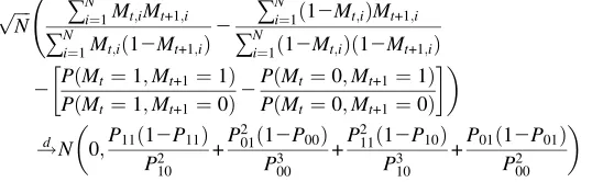
Since weights are being used to calculate the correct percentage of students in each cell, a classical Chi-square test cannot be applied. Following Segal and Yildiz (2006), letMt¼1 if a student misbehaved in yeartand 0 otherwise. We would like
to know whetherMtis independent ofMt+1. DefinePij¼PðMt¼i;Mt+1¼jÞ, where dents who misbehaved in both years is given by1
N+
N
i¼1Mt;iMt+1;i, the fraction of
stu-dents who behaved well on both years is given by 1
N+
N
i¼1ð12Mt;iÞð12Mt+1;iÞ, the
fraction of students who misbehaved only in year t+1 is given by 1
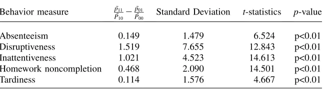
Table 4b presents the results of the independence tests for each behavior measures. The results in Table 4b clearly indicate that the null hypothesis is rejected in all cases.13 Thus, we can conclude that at least for those students who have been in school in the eighth grade and two year afterward, their behavior is not independent across these two years.
The patterns seen in Table 4a are consistent with a model in which students have different costs of behaving well and these costs are stable over time. In such a model, one would expect that children with very low and very high costs of effort would behave the same over time (and the parents would provide small incentives to both types). However, it is not clear whether children with medium costs of behaving well will behave better or worse as they grow older. If, as children grow older, they need to behave better in order to pass to the next grade, then their parents (or their school) would need to provide them with steeper incentives to achieve this goal. If parents’
Table 4a
Behavior Transition Matrices between the 8thand 1990: Percent of Students in Each Category
Absenteeism 1990 Disruptiveness 1990
Behaves well Misbehaves Behaves well Misbehaves
Absenteeism Behaves well 86.4 2.5 Disruptiveness Behaves well 53.5 21.4
8thGrade Misbehaves 9.4 1.7 8thGrade Misbehaves 8.6 16.5
Homework Noncompletion 1990 Inattentiveness 1990
Homework Noncompletion
8thGrade
Behaves well Misbehaves Behaves well Misbehaves
Behaves well 60.5 8.0 Inattentiveness Behaves well 50.1 17.3
Misbehaves 19.7 11.8 8thGrade Misbehaves 13.8 18.8
Tardiness 1990
Behaves well Misbehaves
Tardiness Behaves well 90.9 2.1
8thGrade Misbehaves 6.2 0.9
Number of observations: 4,190.
Notes: The sample was restricted to include individuals who had two teacher evaluations in the eighth grade and in 1990 (not necessarily in the tenth grade). The sample was restricted further to include only students evaluated by teachers that the subject they taught in 1988 and 1990 is known.
Sega
l
benefits from their child’s behavior do not increase with his grade in school, one expects that at least some kids would behave worse as they age. However, if parents’ benefits increase as their child progresses in school, they may decide to supply large incentives for children that previously were supplied with no incentives.
A. Can Behavior Persistence Be Explained By A Stable Environment?
Table 4a and the subsequent tests, presented in Table 4b that reject the independence of behavior across time, indicate that behavior is persistent. However, these tests do not offer any explanation as to the causes. It is possible, though it seems unlikely given the findings reported in Section III, that this persistence in behavior is caused by a stable environment. Below, I investigate this possibility and provide additional evidence for the persistence of behavior.
Table 5 investigates the relation between behavior stability, family background characteristics, and incentives, by presenting the R-squared from linear probability regressions of the different behavior measures on family and school characteristics and on the proxies for the incentives supplied at home and in school, when pooling the data from 1988 and from 1990. The empirical model that is being estimated is
PrðBi;t¼1jXi;Inci;t;Si;t;aiÞ ¼Xib+Inci;tbInc+Si;tbS+ai
whereBi,tis the behavior of individualiin periodt;Xiare the background
character-istics of individuali;14Inci,tare the proxies for the incentives supplied at home and in
school;15Si,tare the characteristics of the school individualiattended in yeart, and Table 4b
Tests for the Independence of Behavior Distributions Between the 8thgrade and 1990
Behavior measure p˜11
˜ P102
˜ p01
˜
P00 Standard Deviation t-statistics p-value
Absenteeism 0.149 1.479 6.524 p<0.01
Disruptiveness 1.519 7.655 12.843 p<0.01
Inattentiveness 1.021 4.523 14.613 p<0.01
Homework noncompletion 0.468 2.090 14.501 p<0.01
Tardiness 0.114 1.576 4.667 p<0.01
Number of observations: 4,190
Notes: The sample was restricted to include individuals who had two teacher evaluations in the eighth grade and in 1990 (not necessarily in the tenth grade). The sample was restricted further to include only students evaluated by teachers for that the subject they taught in 1988 and 1990 is known.
14. The only family background variable for which data is available for both the 1988 and 1990 surveys is family composition.
15. The NELS surveys in 1988 and 1990 do not contain the same questions regarding parental involvement in school and the rules at home. Thus, only questions that were repeated in both survey years were used. Similarly, some of the possible answers in the school administrators survey also have changed between 1988 and 1990, thus only questions that remains the same were used. Moreover, due to low response rates of school administrators in 1990 the questions regarding punishments for class disruptiveness and for verbal abuse of teachers were not used. When adding these variables to the regressions the results reported in Table 5 are essentially the same, the sample size, however, is being reduced by 40 percent.
Table 5
R2from Regressions of each Behavioral Measure on School and Family Characteristics
Dependent Variable: Absenteeism
Dependent Variable: Disruptiveness
Dependent Variable: Homework Noncompletion
Dependent Variable: Inattentiveness
Dependent Variable: Tardiness
Fixed
Effectsa
Background
Characteristicsb
Number of Observations
(1) 0.03 0.05 0.08 0.06 0.03 No Yes 5,050
(2) 0.59 0.65 0.63 0.65 0.55 Yes Yes 5,050
(3) 0.02 0.03 0.06 0.05 0.02 No No 5,412
(4) 0.59 0.65 0.63 0.65 0.55 Yes No 5,412
Notes: The sample was restricted to include individuals who had two teacher evaluations in the eighth grade and in 1990 (not necessarily in the tenth grade). The sample was restricted further to include only students evaluated by teachers that the subject they taught in 1988 and 1990 is known.
a. When individual fixed effects were included in the regressions they were always jointly significant at a level p < 0.01.
b. Background characteristics include a dummy for Black, a dummy for Hispanic, dummies for parental education, family income in 1988, and number of sibling in 1988. The construction of these variables is reported in Table A2 in the Appendix under the family background characteristics section. Other variables included in the regres-sions are a dummy indicating whether the child lived with both parents, a dummy indicating whether parents did not attend school meeting, a dummy indicating whether parents did not talk to the teacher/counselor, a set of dummies indicating whether the parents check if the child has done his homework, require the child to do chores, limit the times spent with friends, limit the time watching TV, and the number of hours per week the child watches TV. The school variables included are a set of dummies indicating whether the child attended Catholic, private religious or private nonreligious school, whether the school is in rural, urban or in the south, and whether discipline is emphasized in school. The construction of these variables is reported in Table A2 in the Appendix.
Sega
l
aiare person-specific fix effects. Obviously,Xibandaicannot be identified jointly.
However, this does not create a problem, because we are mainly interested in check-ing whether a stable environment in the form of given parental and child character-istics can explain the variation in behavior over time.
Columns 2–6 of Table 5 represent regressions where the dependent variable is one of the five behavior measures. Each row presents a specific set of controls. In each cell, the R-squared of a specific regression is reported. For example, the number 0.03 in the upper left corner is the R-squared from a regression of absenteeism on family and school characteristics as well as on school and family rules. The numbers presented in the second row of Table 5 present theR-squared from the same regres-sions when individual fixed-effects are added.
The second row of Table 5 clearly indicates that individual specific traits explain substantial amount of the variation in behavior as the R-squared of the regressions reported in the second row vary between 0.55 for tardiness and 0.65 for disruptive-ness and inattentivedisruptive-ness. However, some of the family characteristics are stable over time (parental education and one’s race) others are highly correlated overtime (paren-tal income and the number of siblings). Moreover, it could be that the incentives pro-vided at home and at school do not vary much over time. Thus, it could be the case that these variables can explain the persistence of behavior. The numbers in the first row of Table 5 indicate that this is not the case.
Person-specific fixed effects are jointly significant for all behavior measures in the regressions reported in Row 2 (p < 0.01). Nevertheless, one cannot directly compare the two models in Rows 1 and 2 since one is not nested in the other. However, it is possible to focus only on the time-varying variables (that is, all variables excluding family background variables) and ask whether person-specific fixed effects belong in the regressions. Rows 3 and 4 in Table 5 report theR-squared from regressions con-trolling only for potentially time-varying variables. The pattern reported in Rows 1 and 2 is repeated. While the R-squared from the time-varying variables (Row 3) ranges from 0.02 for tardiness and absenteeism to 0.08 for homework completion, the R-squared from the regressions in which individual fixed effects were added varies from 0.55 for tardiness to 0.65 for disruptiveness and inattentiveness. Since the models estimated in Row 3 are nested in the models estimated in Row 4, we can now ask whether person-specific effects belong in the regressions. The hypoth-esis that they do not belong in the equations (that is, all person-specific coefficients are jointly zero) is rejected at the conventional significant levels for all the behavior measures (p < 0.01 in all five tests).
The findings reported in Table 5 add further evidence for the persistence of class-room behavior. Although it is possible, and probably likely, that one’s behavior is largely determined within the family, it seems that neither the traditional family background characteristics nor the incentives provided at home (or in school) di-rectly translate into better-behaved children.
see Digman 1990; McCrae and John 1992). These five factors are usually referred to as Extraversion, Agreeableness, Conscientiousness, Neuroticism, and Openness to experience. Conscientiousness, which reflects the tendency to be rule following, task- and goal-directed, planful, and self controlled,16seems to be highly related to behavior in the school. In a recent survey, Roberts et al. (2003) summarize the em-pirical findings regarding the stability of the big five. The evidence in these studies suggests that personality traits are remarkably stable over time, even between child-hood and adolescence, especially after the age of 3. Furthermore, their stability increases even through adolescence and young adulthood, a period of time in which individuals make many life-changing decisions (to marry, have children, career choices, etc.). These patterns do not vary across the five constructs, and conscien-tiousness seems to be the most persistent one (Judge et al. 1999). Thus, the evidence indicates that personality traits seem to be highly stable over time, though not un-changeable.
V. Discussion and Conclusions
Exploiting the information contained in the NELS, this paper inves-tigates the origin and persistence of youth behavior in the classroom. The measures of classroom behavior utilize teacher evaluations of student behavior, avoiding prob-lems associated with self-reporting.
The empirical analysis shows that the behavior of boys in school is persistent, at least after the eighth grade. Most of the variation in behavior can be attributed to un-observed individual heterogeneity, but not to the traditional family background char-acteristics, which include race, parental education and income, number of siblings, and family composition. Nevertheless, the paper demonstrates that observable family and school characteristics have economically, and statistically, meaningful associa-tions to the behavior of boys in school.
The evidence indicates that youth behavior is associated with incentives provided in school, in particular with the degree to which the school emphasizes discipline. The relationships found between the incentives provided at home and child’s behav-ior suggest that youth behavbehav-ior does respond to incentives. However, they also are consistent with a model in which individuals are of different types, where one’s type is one’s costs of behaving well. These relationships are inconsistent with a model where child behavior is only affected by the incentives supplied to him. Moreover, the hypothesis that children’s behavior is independent over time can be rejected. Thus, it is not the case that transitory shocks determine one’s type in a given period. The findings that behavior is persistent over time, and that incentives for good
16. The definitions for the other four traits are as follows (following Roberts et al. 2003). Extroversion refers to the differences across individuals in the tendency to be social active, and assertive. Agreeableness refers to traits that reflect differences across individuals in the tendency to be trusting, modest, altruistic, and warm. Neuroticism, or its converse emotional stability, contracts the experience of anxiety, worry, an-ger, and depression with even-temperedness. Openness to experience reflects individual differences in the tendency of individuals to be open to new ideas, complex, original, and creative.
behavior provided at home and in school cannot account for this persistence, provide supporting evidence to the existence of a stable type.
The goal of this paper is to investigate the possible effectiveness of policies di-rectly targeting noncognitive skills, and classroom behavior in particular. To this end, the analysis in the paper focuses on the relation between youth behavior in the classroom and youth background, and on the persistence of youth behavior. The findings are inconclusive regarding the possible success of policies targeting stu-dent behavior. On the positive side, youth behavior in the classroom is not deter-mined by youth background alone. Hence, directly targeting youth behavior in school may be fruitful. On the negative side, the evidence is consistent with a model in which child’s behavior is determined by his type and the incentive provided to him. Moreover, the evidence suggests that one’s type is fairly stable, at least after the eighth grade. The evidence in psychology on the stability of personality traits supports these findings. Personality traits seem to become more stable as a person gets older. In particular, these traits seem to be changing less during and after adolescence. If one’s costs of behaving well determines one’s success later in life and not only one’s behavior,17 then the relevant policy question is whether one’s type can be changed. A possible positive answer to this question might be found by looking at Catholic schools. In Catholic schools, good behavior is valued for its educational role: ‘‘Sometimes the consequences of one’s choice may be a corrective measure
.the corrective measureis notintended as a punishment, but rather as a reasonable consequence to behavior that is inconsistent with our expectations and rules’’ (St. Anastasia School—Family Handbook 2006-2007).18I find that attending a Catholic school has benefits in terms of behavior even after controlling for the degree to which discipline is emphasized in the school and school rules. One possible interpretation of these results is that targeting classroom behavior for its own sake may be success-ful in changing one’s type for the better and not only one’s behavior. Sorting or just changing one’s behavior as oppose to one’s type are the other possible interpretations. The findings presented in this paper do not rule out the possibility that one’s costs of behaving well can change. They do not even indicate that parents (and perhaps schools) are not making continuous investments in order to reduce children’s costs of behaving well. As with any investment, investment in noncognitive skills would be more profitable the longer one has to enjoy its fruits. Thus, it is possible that sub-stantial part of the investment in reducing child’s costs of behaving well on parents’ part (and may be on school’s part too) has been made in the past. Therefore, the sta-bility of one’s type, from the eighth grade onward, may reflect small investments op-timally made in adolescence.
The evidence presented in this paper does not allow for an unambiguous conclu-sion regarding the possible effectiveness of policies that would directly target class-room behavior. While it is possible that such policies would be successful, as behavior is not solely determined by one’s background, adolescence appears to be too late. It is possible that in younger age behavior is more compliant, and hence
17. The findings in Segal (2005) are consistent with the interpretation that classroom behavior is a proxy for one’s traits.
18. St. Anastasia School—Family Handbook 2006-2007 can be found at: http://www.stanastasiawaukegan. org/.
targeting behavior earlier in life may be successful. Moreover, the evidence does not rule out the possibility that targeting behavior for its own sake in the school would be successful. More data on childhood and adolescent behavior might help shed light on some of these open questions.
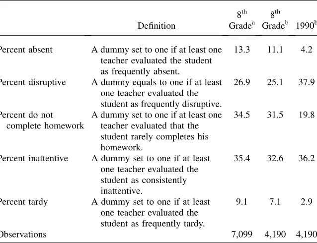
Table A1
Summary Statistics: Behavior in the eighth Grade and in 1990
Definition
8th Gradea
8th
Gradeb 1990b
Percent absent A dummy set to one if at least one teacher evaluated the student as frequently absent.
13.3 11.1 4.2
Percent disruptive A dummy equals to one if at least one teacher evaluated the student as frequently disruptive.
26.9 25.1 37.9
Percent do not complete homework
A dummy set to one if at least one teacher evaluated that the student rarely completes his homework.
34.5 31.5 19.8
Percent inattentive A dummy set to one if at least one teacher evaluated the student as consistently inattentive.
35.4 32.6 36.2
Percent tardy A dummy set to one if at least one teacher evaluated the student as frequently tardy.
9.1 7.1 2.9
Observations 7,099 4,190 4,190
Notes: a. The sample was restricted to include only those students who had two teacher evaluations in the eighth grade, and had valid data for family background characteristics, family rules variables, and school characteristics variables (the variables are described in Table A2 in the Appendix).
b. The sample was restricted to include individuals who had two teacher evaluations in the eighth grade and in 1990 (not necessarily in the tenth grade). The sample was restricted further to include only the teachers that the subject they taught in 1988 and 1990 is known.
Table A2
Data Description and Variable Construction
Variable
Percent in
Category Definition
Family Background Characteristics
Black 9.6 A dummy equals to one if the person is Black
non-Hispanic.
Hispanic 8.1 A dummy equals to one if the person is Hispanic.
White 82.3 A dummy equals to one if the person is non-Black
non-Hispanic.
Father high school dropout 14.6 The set of dummies were constructed from the studentsÕ
answers to the questions regarding their parentsÕ/ guardiansÕeducation. In case the data was missing, parentsÕ/guardiansÕanswers were used. In case of missing data about one of the parents and the parent/guardian reported that he/she is the only guardian, the value for the other parent was set to zero. The categories are: High School Dropout—no high school diploma, High School Graduate —has a high school diploma (does not include GED), and College Degree or More—Bachelor degree or more. If the answer is in a given category the dummy is set to one.
Father high school graduate 53.3
Father college graduate or more 29.2
Mother high school dropout 13.3
Mother high school graduate 61.9
Mother college graduate or more 24.4
Income (in $)—(mean) 41,590 The variable was constructed using the parentsÕ/guardiansÕ
answer to the question: ‘‘What was your total family income from all sources in 1987?’’ The answers were given in categories. For each category, the midpoint was taken to construct a linear measure.
Does not live with both parents 31.0 The variable was constructed using both studentsÕand parentsÕ1988 survey. The dummy is equal to zero if the youth live with both parents and equal to one otherwise.
(continued)
808
The
Journal
of
Human
Table A2 (continued)
Variable
Percent in
Category Definition
Number of siblings (mean) 2.2 The variable was constructed using the studentsÕresponses and when it was missing the data was taken from parentsÕ/guardiansÕresponse. The data was truncated at six siblings or more.
Has dropouts siblings 8.6 A dummy equals to one if the individual has at least one sibling who dropped out of high school.
Has high school graduates siblings 28.1 A dummy equals to one if the individual has at least one sibling who graduated from high school.
Only child 6.1 A dummy equals to one if the individual is an only child.
Number of older siblings (mean) 1.2 Number of older siblings, the data is truncated at six.
Youngest child 34.7 A dummy equals to one, if the number of siblings older
than the individual is equal to the number of siblings the individual has.
Father works 92.0 A dummy equals to one if the father/guardian worked in
1988. The variable was constructed using both studentsÕ
and parentsÕ1988 surveys.
Mother works 90.9 A dummy equals to one if the mother/guardian worked in
1988. The variable was constructed using both studentsÕ
and parentsÕ1988 surveys.
Family Rules All Variables in category were constructed using 1988
student survey.
Parents didn’t attend school meetings 47.9 A dummy equals to one if the parentsdid notattend school meetings.
Parents didn’t talk to teacher/counselor 37.0 A dummy equals to one if the parentsdid nottalk to Teacher/Counselor.
Parents didn’t visited classes 72.3 A dummy equals to one if the parentsdid notvisit classes.
Sega
l