Full Terms & Conditions of access and use can be found at
http://www.tandfonline.com/action/journalInformation?journalCode=ubes20
Download by: [Universitas Maritim Raja Ali Haji] Date: 12 January 2016, At: 17:33
Journal of Business & Economic Statistics
ISSN: 0735-0015 (Print) 1537-2707 (Online) Journal homepage: http://www.tandfonline.com/loi/ubes20
Forecasting Professional Forecasters
Eric Ghysels & Jonathan H. Wright
To cite this article: Eric Ghysels & Jonathan H. Wright (2009) Forecasting Professional Forecasters, Journal of Business & Economic Statistics, 27:4, 504-516, DOI: 10.1198/ jbes.2009.06044
To link to this article: http://dx.doi.org/10.1198/jbes.2009.06044
Published online: 01 Jan 2012.
Submit your article to this journal
Article views: 246
View related articles
Forecasting Professional Forecasters
Eric G
HYSELSDepartment of Finance, Kenan–Flagler School of Business and Department of Economics, University of North Carolina, Gardner Hall CB 3305, Chapel Hill, NC 27599-3305 (eghysels@unc.edu)
Jonathan H. W
RIGHTDepartment of Economics, Johns Hopkins University, Baltimore, MD 21218 (wrightj@jhu.edu)
Surveys of forecasters, containing respondents’ predictions of future values of key macroeconomic vari-ables, receive a lot of attention in the financial press, from investors and from policy makers. They are apparently widely perceived to provide useful information about agents’ expectations. Nonetheless, these survey forecasts suffer from the crucial disadvantage that they are often quite stale, as they are released only infrequently. In this article, we propose MIDAS regression and Kalman filter methods for using asset price data to construct daily forecasts of upcoming survey releases. Our methods also allow us to predict actual outcomes, providing competing forecasts, and allow us to estimate what professional forecasters would predict if they were asked to make a forecast each day, making it possible to measure the effects of events and news announcements on expectations.
KEY WORDS: Forecast evaluation; Kalman filter; Mixed frequency data sampling; News announce-ments; Survey forecasts.
1. INTRODUCTION
Surveys of professional forecasters are released, typically on a quarterly or monthly basis, containing respondents’ predic-tions of key macroeconomic variables. These releases get wide coverage in the financial press and many of the forecasters be-ing surveyed have a large clientele base paybe-ing considerable sums of money for their services. The sources and methods that these forecasters use are somewhat opaque, but a large quan-tity of their information is economic news that is in the public domain. Through the market process of price discovery, this economic news is also impounded in financial asset prices.
In this article, we propose methods for using asset price data to construct daily forecasts of upcoming survey releases. Our methods also allow us to estimate what professional forecasters would predict if they were asked to make a forecast each day, making it possible to measure the effects of events and news announcements on expectations. The empirical models we con-struct also readily become competing forecasting models and we show that they indeed provide accurate forecasts of the ac-tual outcomes, competing with survey forecasts, while being more timely.
There are various reasons why we are interested in measur-ing professional forecasters’ expectations at a daily frequency. First, agents’ expectations are of critical importance to policy makers, and policy makers apparently perceive surveys of fore-casters to be providing useful information about those expecta-tions. Monetary policy communications, such as the minutes of the Federal Open Market Committee, frequently point to survey expectations of inflation. Policy makers, monitoring the econ-omy in real time, would presumably like to be able to measure these expectations at a higher frequency than the current in-frequent survey dates. The methods that we propose allow us to measure expectations immediately before and after a spe-cific event (e.g., macroeconomic news announcements, Federal Reserve policy shifts, or major financial crises) and so mea-sure the impact of such events on agents’ expectations. Second, expectations in a multiagent economy involve “forecasting the
forecasts of others” (to paraphrase Townsend1983) and, there-fore, private sector agents would likewise also wish to obtain higher frequency measures of others’ expectations. A third rea-son (closely related to the first two) is that surveys may be (ap-proximately) rational or efficient forecasts of future economic data and may thus contain information for policy makers not just about agents’ expectations, but also about likely future out-comes. In this article we do not, however, make an assumption that surveys represent rational conditional expectations.
While there are many reasons for measuring professional forecasters’ expectations at high frequency, the task itself, as noted before, is not so trivial. One may first of all wonder which data would be most suitable to use. The task is very much re-lated to the construction of leading indicators, or the extraction of a common factor as in, for example, Stock and Watson (1989, 2002). We could use low-frequency macroeconomic data, or high-frequency asset price data. But the latter will allow us to make predictions at any point in time, which is our goal in this article. Thus, in this article we use daily asset price data.
A priori, it is not clear how to use daily financial market data to formulate a parsimonious model. The challenge of formu-lating models to accomplish these tasks is that financial data are abundant and arrive at much higher frequency than the re-leases of macroeconomic forecasts. It quickly becomes obvious that, unless a parsimonious model can be formulated, there is no practical solution for linking the quarterly forecasts to daily fi-nancial data. A simple linear regression will not work well as it would entail estimating a large number of parameters and the estimation uncertainty would nullify any underlying predictable patterns that might exist. Matters are further complicated by the fact that there is some fuzziness in the timing of the surveys: although we have a notional date for each survey (the dead-line for submission of responses), we have no way of knowing
© 2009American Statistical Association
Journal of Business & Economic Statistics October 2009, Vol. 27, No. 4 DOI:10.1198/jbes.2009.06044 504
Ghysels and Wright: Forecasting Professional Forecasters 505
whether the forecasters actually formed their predictions on the survey deadline date or several days earlier. To allow for this we might want to use more than two months of data. We resolve the challenge by using mixed data sampling, or MIDAS regression models, proposed in the recent work of Ghysels, Santa-Clara, and Valkanov (2005,2006). MIDAS regressions are designed to handle large high-frequency datasets with judiciously chosen parameterizations, tightly parameterized yet versatile enough to yield predictions of low frequency forecast releases with daily financial data.
In addition to using these regression models to predict up-coming survey releases, we consider a more structural approach in which we use the Kalman filter to estimate what forecasters would predict if they were asked to make a forecast each day, treating their forecasts as “missing data” to be interpolated (see, e.g., Harvey and Pierse1984; Harvey1989; Bernanke, Gertler, and Watson1997). As a by-product, this also gives forecasts of upcoming releases. Again, however, we have to contend with the fact that although we have a notional date for each survey, agents likely formed their expectations sometime earlier. Again, we resolve this problem by using mixed data sampling methods. In our empirical work we use the median forecasts of out-put growth, inflation, unemployment, and interest rates, from the Survey of Professional Forecasters (Croushore1993). The financial market data that we use to predict these forecasts are daily changes in interest rates. We find that these asset price changes give us considerable predictive power for upcoming Survey of Professional Forecasters releases. Having obtained estimates of agents’ daily forecasts, we can then relate these to macroeconomic news announcements. For example, we can measure the average effect of a nonfarm payrolls announcement that is 100,000 better-than-expected on agents’ forecasts. We find economically meaningful and statistically significant news impact estimates.
The remainder of this article is organized as follows. In Sec-tion2we present a theoretical framework that succinctly repre-sents the salient features of predicting forecasters with financial data and present the empirical methods. Empirical results ap-pear in Section3. Section 4discusses the impact of news on expectations. Section5concludes the article.
2. FORECASTING AND FINANCIAL MARKET SIGNALS
In this section we show, in a very stylized setting, how if as-set prices and forecasts both respond to news about the state of the economy, we can use asset returns to glean high-frequency information about agents’ forecasts. As we want to keep the model in this section simple, we make compromises with re-gards to generality and do not aim at matching all salient data features that will appear in our empirical analysis. We also present the empirical methods, both regression-based and Kalman filter, as they relate to the stylized model.
Assume that we observe forecasts of some future macro-economic variableyt (e.g., inflation four quarters hence) once a quarter and suppose, for simplicity, that these are observed on the last day of each quarter. Moreover, let the underlying process forytbe AR(1):
yt+1=a0+a1yt+εt+1. (1)
Let ftt+h denote the forecast ofyt+h made on the last day of
quartert. We focus onhperiod ahead forecasts as professional forecasters produce multiple period ahead predictions, which are in turn of most interest to forward-looking policymakers or investors. If the forecaster knows the DGP, knowsytat the end
of quartert(when the forecast is being made), and is construct-ing a rational forecast then this h-quarter-ahead forecast will be:
which is related to the previoush-quarter-ahead forecast and the shockεtas follows:
We are interested in predictingftt+hat some time between the end of quartert−1 and the end of quartert.During the quarter news is released pertaining to the macroeconomic variableyt,
which is impounded into financial asset returns. Although the errorsεt occur quarterly, we construct a fictitious set of daily
shocksεt≡ldt=lt−1+1vd, whereltdenotes the last day of
quar-tert. While there are many financial assets traded, we focus on a single asset and assume that its price on dayτ relates to the fictitious shocks as follows:
wherep0t is the price at the beginning of the quarter t. Equa-tion (4) tells us that daily prices provide a noisy signal of the underlying economic shocks. Assume that the fictitious shocks
vd are Gaussian with mean zero and varianceσv2 and that the
noise is also Gaussian with mean zero and varianceσw2 and is orthogonal to thevd process. We make these assumptions for
convenience, but will comment on them later. The two related problems we then consider are: (1) predictingftt+hduring quar-tert with concurrent and past daily financial market data via a regression model, or (2) treating agents’h-quarter-ahead ex-pectationsduringthe quarter as “missing” values of a process only observed at the end of the quarter. There is a fundamen-tal difference between predictingftt+h, during the quarter, and
“guessing”ϕτh, the unobservedh-quarter-ahead expectation on dayτ. The former is a prediction problem that can be formu-lated via a regression, whereas the latter is a filtering problem.
Asset prices embed both forecasts of future (macro) factors and also prices of risk, and there is substantial evidence in the finance literature that the prices of risk are time-varying. Our simple reduced form model does not attempt to split these out. One remedy would be to replace the “plain” return series used in our model by so-called economic tracking portfolios (see, e.g., Breeden, Gibbons, and Litzenberger 1989, or more re-cently Lamont 2001 and Christoffersen, Ghysels, and Swan-son 2002). Lamont (2001) in particular, constructed tracking portfolios for future economic variables, and used only the un-expected component of returns (not total returns) in construct-ing the trackconstruct-ing portfolios. In principle, one could use trackconstruct-ing
506 Journal of Business & Economic Statistics, October 2009
portfolio returns and this might further improve the forecast-ing performance that we document in this article, but construct-ing these portfolios involves estimation error and evidence on their out-of-sample forecasting power is mixed. Besides the ad-ditional complications pertaining to estimation error, it should also be noted that data vintage issues play a role in the construc-tion of economic tracking portfolios (see, e.g., Christoffersen, Ghysels, and Swanson2002for further discussion). The virtue of using plain return series is, therefore, the avoidance of addi-tional estimation error and data revision issues. The downside is that we cannot separate movements in risk premia from ex-pected future macro factors that both affect the return processes feeding into our prediction models.
2.1 The Regression Approach
From Equation (4), the partial sums process Sτ = τ
d=lt−1+1vd behaves like a random walk and, therefore, the
asset pricepτt behaves like a random walk plus noise (in prac-tice stock prices are not a random walk, but this is one of our simplifying assumptions). To predict ftt+h, we would like to knowεt+1, and the best predictor on dayτ would beSτ which is not observed but can be extracted from asset returns. In par-ticular, inAppendixwe show that conditional linear prediction given daily returns, denotedP can be approximated as:
P[ftt+h|rd,d=lt−1+1, . . . , τ] [see Equation (A.2) in theAppendix] andrdis the asset return on daydfor dayslt−1+1,. . .,τ during quartert.
The stylized model presented so far is based on a number of simplifying assumptions. It is worth discussing some of the critical assumptions and how they can be relaxed. Firstly, the above analysis assumes that forecasters have rational expec-tations and know the DGP. The analysis in the remainder of the article will not exclude the possibility of rational forecast-ing, and that would clearly strengthen the motivation for real-time forecasting of the forecasters. Nevertheless, our empirical model does not rely on such an assumption and, throughout this article, we remain strictly agnostic about the rationality of fore-casters’ expectations.
Secondly, to derive Equation (5) we assumed Gaussian er-rors. The resulting prediction formula only depended on the signal to noise ratio q and the linear prediction is optimal in a MSE sense. With the Gaussian distributional assumptions, we are, in fact, in the context of the Kalman filter, the topic of the next subsection. Here we consider Equation (5) as a linear pro-jection or regression equation. Obviously, this regression equa-tion is tightly parameterized because the analysis has been kept simple for the purpose of exposition. In particular, the processyt
was assumed to be a random walk and this yielded convenient formulas in this example. In practice, we prefer to have reduced
form regressions that do not explicitly hinge on the specifics of the DGP.
Our empirical specification uses regression models for pre-dictingftt+h. Letdtdenote the survey deadline date for quartert:
survey respondents submit their forecasts on or before this day: the survey results are released a few days later. We suppose that the researcher wishes to forecastftt+husing asset return data on days up to and including dayτ. Our forecasting model is:
ftt+h=α+ρftt−−11+h+ vey deadline date, about one month earlier, and about two months earlier, respectively. Equation (6) uses mixed frequency data:ftt+h andftt−−11+h are observed at the quarterly frequency,
t=2, . . . ,T, while the returns are at the daily frequency, but there is only one observation of the distributed lag of daily re-turns,γ (L)rjτ, in each quarter. Hence, as suggested by Equa-tion (5), asset returns up to a fracEqua-tionθ of the time from the quartert−1 survey deadline date to the quartertsurvey dead-line date are used to predict the quarter t survey. We run a different regression for eachθ and so should strictly put aθ -subscript onα,{βj}jn=A1,ρ, andγ (L)in Equation (6), but do not do so, in order to avoid excessively cumbersome notation. In or-der to identifyβjin this equation, we constrain the polynomial
γ (L)to have weights that add up to one. Following Ghysels, Sinko, and Valkanov (2006) we use a flexible specification for γ (L)with only two parameters, κ1 andκ2, using their “Beta Lag” specification. It should be noted that Ghysels, Sinko, and Valkanov (2006) discussed various schemes besides the Beta Lag specification. Similar results can be obtained with other polynomials, but the beta lag specification is convenient be-cause it can capture the hump-shaped weighting function that we consistently find in empirical applications with just two pa-rameters.
We consider three MIDAS regression models for the pre-diction of ftt+h. The first, which we refer to as model M1, is simply given by Equation (6) with unknown parametersα,
{βj}nj=A1, ρ, κ1 and κ2. The second, model M2, imposes that κ1=κ2=1, implying that the weights in γ (L) are equal. In this case,γ (L)rjτ is simply the average return over thenl days up until dayτ andγ (L)=nl
j=1(1/nl)Lj−1. Lastly, we consider
an equal-weighted MIDAS regression in which the average re-turns from daydt−1to dayτ are used to predict the upcoming release, i.e.,γ (L)=nτ
j=1(1/nl)Lj−1 and nτ =τ −dt−1. We refer to this as model M3. The difference between models M2 and M3 is that model M2 has a fixed lag length parameter,nl,
while model M3 will always use returns from exactly daydt−1 to dayτ. We estimate MIDAS models M2 and M3 by OLS and M1 by nonlinear least squares.
Ghysels and Wright: Forecasting Professional Forecasters 507
2.2 The Filtering Approach
We now turn to the second problem, namely how to ex-tractϕτh. For this, it is very natural to specify and estimate a state space model using the Kalman filter to interpolate respon-dents’ expectations (see, e.g., Harvey and Pierse1984; Harvey 1989; Bernanke, Gertler, and Watson1997). It is worth noting that the regression approach of the previous subsection can be viewed as less “structural” in the sense that we do not need to specify an explicit state space model. The Kalman filter applies to homoscedastic Gaussian systems, assumptions we make here for analytic convenience. To be specific, let us reconsider Equa-tion (3) and apply it to a daily setting:
ϕτh≈ϕτh−1+ ˜avτ. (7) The shocksvτ are not directly observable, only the returns are. The above equation, therefore, holds the ingredients for a state space model to determineϕτh, namely daily returns are a noisy signal of daily changes inϕτh:
The Kalman filter applies to homoscedastic Gaussian sys-tems and this assumption is clearly inadequate for financial data. However, the Kalman filter provides optimal linear predic-tion even with non-Gaussian errors. We consider two thought-experiments that go beyond the simple stylized example. The first is that forecasters form expectations each day, but only send these expectations into the compilers of the survey once a quarter, on survey deadline dates. Thus, we observe respon-dents’ expectations on survey deadline dates, but these expec-tations must be interpolated on all other days. We letϕτh de-note the respondents’h-quarter-ahead expectations on daytand write the following model nal variance-covariance matrix. This model is clearly a lin-ear Gaussian model in state-space form withϕτhas the unob-served state, Equation (10) as the transition equation, and Equa-tions (9) and (11) as the elements of the measurement equation. Note that we avoid here a direct mapping between the parame-ters of the stylized model. Instead, we proceed with a generic state space model, similar to the generic MIDAS regressions considered in the previous section.
As discussed earlier, there is some uncertainty about the ex-act timing of respondents’ expectations that it seems we should allow for. We can do so by amending Equation (11) to specify instead that
ftt+h=γ (L)ϕdh
t, (12)
whereγ (L)is a MIDAS polynomial. Thus the second thought-experiment is that individual respondents form their expecta-tions each day, but that some of these get transmitted to the compilers of the survey faster than others, with the compilers
of the survey using the latest numbers from each respondent to construct the survey releases once a quarter, on survey deadline dates. Our objective is to back out our estimates of respondents’ underlying expectations given byϕτh. Of course, the model in which surveys correspond exactly to respondents’ expectations on survey deadline dates is nested within this specification, as we can specify thatκ1=1 andκ2= ∞, implying thatγ (L)=1. We refer to the simple Kalman filter model [Equations (9), (10), and (11)] as model K1. We refer to the MIDAS Kalman fil-ter model [Equations (9), (10), and (12)] as model K2. In either case, we can use the Kalman filter to find maximum-likelihood estimates of the parameters, giving filtered estimates ofϕτhand forecasts of ftt+h (made a fraction θ of the way through the prior intersurvey period) as by-products. We can also use the Kalman smoother to obtain estimates ofϕhτ conditional on the entire dataset. The simple Kalman filter model has been used in several mixed-frequency applications such as Zadrozny (1990), who was concerned with the problem of using observed quar-terly GNP and other monthly data to interpolate monthly GNP numbers. But the MIDAS Kalman filter model is new and its greater flexibility may be helpful in our application of interpo-lating survey predictions at the daily frequency.
3. EMPIRICAL RESULTS
The survey that we consider in the empirical work is the Survey of Professional Forecasters (SPF), conducted at a quar-terly frequency. The respondents include Wall Street financial firms, banks, economic consulting groups, and economic fore-casters at large corporations. Prior to 1990, it was a joint project of the American Statistical Association and the National Bu-reau of Economic Research; now it is run by the Federal Re-serve Bank of Philadelphia. We use median SPF forecasts of real GDP growth, CPI inflation, three-month T-Bill yields, and the unemployment rate at horizons one-quarter through four-quarters ahead. Real GDP growth and CPI inflation are con-structed as the annualized growth rates from quarter t−1 to quartert+h, wheretis the quarter in which the survey is taken andhis the horizon of the forecast (h=1,2,3,4). Three-month T-Bill yields and the unemployment rate are simply expressed in levels. In the notation of the previous section,ftt+hrefers to the forecast made in the quartertSPF forecast for any one of these variables in quartert+hand our forecasting models are the MIDAS and Kalman filter models exactly as defined earlier. We start with the forecasts made in 1990Q3 and end with fore-casts made in 2005Q4 for a total of 62 forefore-casts. For each of these forecasts we have the survey deadline dates that are about in the middle of each quarter. The survey deadline date is not the date that the survey results are released, but is the last day that respondents can send in their forecasts. We do not use SPF forecasts made before 1990Q3 because we do not have the as-sociated survey deadline dates. Besides, the use of a relatively recent sample minimizes issues of structural change that seem to be very important using data that spans earlier time periods (Ang, Bekaert, and Wei2007and Stock and Watson2003). In the working paper version of the article we also report results covering the Consensus Forecasts, a survey that is conducted at a monthly frequency by Consensus Economics (see Ghysels and Wright2006).
508 Journal of Business & Economic Statistics, October 2009
We can use daily asset prices to predict the upcoming re-leases of the survey, using MIDAS regression models M1, M2, and M3, or our Kalman filter models K1 and K2. We con-sider models with the following daily asset returns: (a) the daily changes in three-month and ten-year Treasury yields, and (b) the daily change in two-year Treasury yields, using the con-stant maturity yields (H-15 release). The number of assets,nA,
is thus either 1 or 2 and these assets represent the level and/or slope of the yield curve. Results with other assets are reported in Ghysels and Wright (2006).
3.1 MIDAS Regression Results
In MIDAS models M1 and M2, the lag lengthnl is a fixed parameter that we set to 90. As our data are at the business day frequency, this corresponds to substantially more than one quarter of data. We do this because we have no way of knowing whether the forecasters actually formed their predictions on the survey deadline date or several days earlier, and because pre-liminary investigation revealed that this choice ofnl generally
gave the best empirical fit.
We evaluate the forecasts by comparing the in-sample and pseudo-out-of-sample root mean-square prediction error (RM-SPE) of each of the models M1, M2, M3, K1, and K2, used to predict the upcoming survey release, relative to the RMSPE from fitting an AR(1)to the survey releases [an “AR(1)” focast]. The empirical results for predictors (a) and (b) are re-ported in Tables1and2, respectively. Both tables give the in-sample and pseudo-out-of-in-sample RMSPE of models M1, M2, M3, K1, and K2, used to predict the upcoming survey release, relative to the AR(1)benchmark, forθ=1,2/3,1/3. The first observation for out-of-sample mean square prediction is the first observation in 1998, with parameters estimated only us-ing data from 1997 and earlier, and prediction then continues from this point on in the usual recursive manner, forecasting in each period using data that were actually available at that time. Note that because we are working with asset price data and sur-vey forecasts (rather than actual macroeconomic realizations), we have no issues of data revisions to contend with; the out-of-sample forecasting exercise is a fully real-time forecasting exercise.
We first discuss the simple regression results (models M1, M2, and M3). The in-sample relative RMSPEs from MIDAS models M1, M2, and M3 are by construction less than or equal to one, and are generally well below one. Not surprisingly, rel-ative RMSPEs are higher in the pseudo-out-of-sample forecast-ing exercise. Survey forecasts of the unemployment rate and T-Bill yields appear to be generally the most predictable out-of-sample, but out-of-sample relative RMSPEs are in many cases below one for GDP growth and CPI inflation forecasts as well. The results are similar for both predictors, but the better out-of-sample results mostly appear to obtain for predictors (a) (the daily changes in the three-month and ten-year Treasury yields). On average, across all four variables and all four horizons, the pseudo-out-of-sample relative RMSPE from MIDAS model M1 withθ=1 and predictors (a) is 0.77. However, using predic-tors (b) (the daily changes in two-year Treasury yields alone) generally gives better out-of-sample predictions for real GDP growth forecasts, which is consistent with the work of Ang, Pi-azzesi, and Wei (2006) who found that the level of short-term
interest rates alone has more predictive power for growth than any term spread.
Even though MIDAS model M1 involves estimation of two additional parameters, it generally gives smaller out-of-sample RMSPEs than models M2 or M3. Thus, perhaps in part because the surveys represent agents’ beliefs at a substantial lag relative to the survey deadline date (a lag that furthermore varies by respondent), allowing for nonequal weights inγ (L)appears to result in improved forecasting performance. The improvement is quite substantial in many cases.
Not surprisingly, the relative RMSPE is generally somewhat smaller for forecasts made using asset price data up through the survey deadline date (θ=1) than for forecasts made earlier in the intersurvey period (θ=2/3,1/3).
3.2 Kalman Filtering Results
We next discuss the results using the Kalman filter (models K1 and K2). The patterns are similar. Again, the best results ob-tain when predicting the forecasts for three-month T-Bill yields and the unemployment rate, and when using predictors (a). Model K2, which allows for surveys to represent respondents’ beliefs at a substantial lag relative to the survey deadline date, generally gives smaller out-of-sample RMSPEs than model K1, and the improvement is quite substantial in many cases, even though it involves estimation of two additional parameters. This reinforces the evidence that surveys represent agents’ beliefs at a considerable lag to the survey deadline date.
Models K1 and K2 on average give slightly less good fore-casts of what the upcoming survey release is going to be than the reduced form MIDAS regression models M1, M2, and M3. Nonetheless, they have the useful feature of allowing us to es-timate forecasters’ expectations on a day-to-day basis, [ϕτh in the notation of Equation (9)] and these estimates can be ei-ther conditional on past data (filtered estimates) or the whole sample (smoothed estimates). We cannot precisely accomplish these tasks with the reduced form MIDAS regression models.
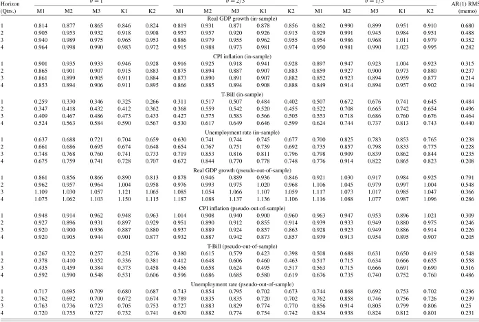
As an illustration, in Figure1, we show the time series of Kalman smoothed estimates of two-quarter-ahead real GDP growth expectations from models K1 and K2, using predic-tors (a), over the period since January 1998. In the compan-ion working paper (Ghysels and Wright2006) we also reported Kalman filtered estimates. SPF releases of actual two-quarter real GDP growth expectations are also shown on the figure (dated as of the survey deadline date). The Kalman filter es-timates jump on each survey deadline date as the information from the survey becomes incorporated in the model, but the jumps are quite a bit smaller in magnitude than the revisions to the survey forecasts, consistent with the results in Tables1and2 on the RMSPE of the Kalman filter forecasts relative to that of the AR(1)benchmark. As expected, the Kalman smoothed esti-mates adjust more smoothly than the Kalman filtered estiesti-mates.
3.3 Parameter Estimates
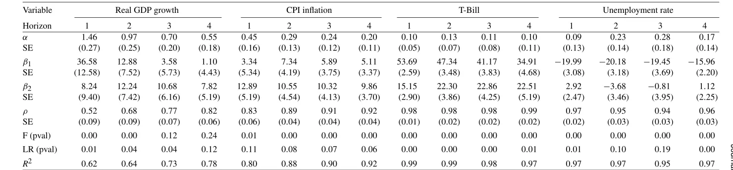
Across all combinations of predictors, forecast horizons, and models that we have estimated, the number of parameters is very large. As an illustration of these parameter estimates, Ta-ble3 reports the estimates from fitting model M1 to the SPF
Gh
ysels
and
Wr
ight:
F
orecasting
Prof
essional
F
orecasters
509
Table 1. In- and pseudo-out-of-sample root mean square error of predictions of the SPF
θ=1 θ=2/3 θ=1/3
Horizon AR(1)RMSE
(Qtrs.) M1 M2 M3 K1 K2 M1 M2 M3 K1 K2 M1 M2 M3 K1 K2 (memo)
Real GDP growth (in-sample)
1 0.814 0.877 0.865 0.846 0.824 0.819 0.931 0.871 0.878 0.856 0.862 0.990 0.899 0.951 0.910 0.680
2 0.905 0.953 0.932 0.918 0.908 0.957 0.957 0.920 0.926 0.915 0.929 0.991 0.945 0.984 0.951 0.488
3 0.940 0.989 0.975 0.965 0.953 0.886 0.979 0.955 0.962 0.955 0.954 0.986 0.968 1.011 0.979 0.352
4 0.964 0.998 0.990 0.983 0.972 0.915 0.988 0.973 0.981 0.974 0.950 0.981 0.990 1.023 0.995 0.282
CPI inflation (in-sample)
1 0.901 0.935 0.933 0.946 0.928 0.916 0.925 0.918 0.941 0.928 0.897 0.947 0.923 1.004 0.923 0.315
2 0.865 0.901 0.907 0.915 0.883 0.875 0.894 0.887 0.907 0.883 0.859 0.927 0.900 0.973 0.880 0.237
3 0.861 0.899 0.905 0.911 0.884 0.873 0.890 0.891 0.907 0.882 0.852 0.923 0.894 0.959 0.877 0.214
4 0.853 0.894 0.906 0.911 0.895 0.866 0.885 0.894 0.908 0.888 0.849 0.914 0.894 0.957 0.902 0.194
T-Bill (in-sample)
1 0.259 0.330 0.346 0.325 0.266 0.311 0.517 0.507 0.484 0.402 0.507 0.672 0.676 0.741 0.645 0.484
2 0.347 0.418 0.432 0.412 0.362 0.368 0.559 0.542 0.520 0.455 0.522 0.708 0.665 0.742 0.654 0.496
3 0.409 0.467 0.486 0.473 0.433 0.427 0.575 0.583 0.566 0.505 0.553 0.718 0.686 0.760 0.676 0.464
4 0.524 0.563 0.584 0.590 0.567 0.530 0.617 0.649 0.646 0.599 0.624 0.744 0.737 0.813 0.743 0.440
Unemployment rate (in-sample)
1 0.637 0.688 0.721 0.704 0.659 0.630 0.741 0.744 0.745 0.677 0.700 0.825 0.783 0.853 0.765 0.238
2 0.661 0.686 0.695 0.674 0.648 0.654 0.767 0.751 0.739 0.692 0.735 0.857 0.798 0.833 0.775 0.228
3 0.748 0.768 0.760 0.741 0.733 0.719 0.853 0.816 0.811 0.796 0.798 0.909 0.839 0.862 0.844 0.235
4 0.675 0.759 0.741 0.728 0.707 0.672 0.844 0.770 0.778 0.748 0.776 0.914 0.822 0.865 0.823 0.208
Real GDP growth (pseudo-out-of-sample)
1 0.861 0.856 0.866 0.890 0.813 0.878 0.946 0.889 0.936 0.846 0.921 1.030 0.917 0.984 0.925 0.791
2 0.962 0.957 0.964 1.004 0.958 0.976 0.993 0.975 1.020 0.968 1.106 1.045 0.979 0.997 1.004 0.548
3 1.109 1.030 1.057 1.121 1.065 1.085 1.054 1.066 1.107 1.059 1.117 1.073 1.017 0.985 1.047 0.366
4 1.075 1.062 1.103 1.150 1.115 1.187 1.088 1.137 1.136 1.106 1.116 1.088 1.077 0.987 1.096 0.286
CPI inflation (pseudo-out-of-sample)
1 0.948 0.914 0.962 0.948 0.963 1.014 0.908 0.940 0.900 0.960 0.963 0.947 0.953 0.896 1.021 0.309
2 0.927 0.896 0.931 0.897 0.929 0.951 0.890 0.912 0.855 0.914 0.939 0.933 0.949 0.880 0.975 0.246
3 0.920 0.900 0.936 0.887 0.880 0.937 0.889 0.924 0.857 0.863 0.928 0.923 0.949 0.886 0.914 0.226
4 0.920 0.905 0.944 0.901 0.877 0.932 0.887 0.942 0.873 0.857 0.939 0.913 0.954 0.895 0.907 0.205
T-Bill (pseudo-out-of-sample)
1 0.267 0.322 0.257 0.251 0.276 0.380 0.615 0.579 0.423 0.398 0.508 0.688 0.631 0.650 0.619 0.548
2 0.378 0.410 0.352 0.336 0.381 0.412 0.648 0.606 0.460 0.463 0.517 0.715 0.634 0.666 0.655 0.558
3 0.435 0.459 0.384 0.373 0.458 0.456 0.658 0.624 0.495 0.517 0.563 0.715 0.666 0.691 0.690 0.516
4 0.592 0.590 0.548 0.531 0.606 0.596 0.686 0.685 0.580 0.619 0.676 0.735 0.740 0.752 0.760 0.486
Unemployment rate (pseudo-out-of-sample)
1 0.717 0.695 0.709 0.680 0.687 0.743 0.854 0.795 0.702 0.673 0.744 0.868 0.692 0.753 0.702 0.236
2 0.762 0.692 0.700 0.672 0.674 0.789 0.835 0.835 0.720 0.702 0.762 0.858 0.746 0.756 0.726 0.239
3 0.763 0.736 0.723 0.705 0.753 0.727 0.883 0.829 0.774 0.770 0.856 0.914 0.805 0.799 0.806 0.25
4 0.720 0.755 0.727 0.732 0.741 0.670 0.882 0.774 0.754 0.742 0.834 0.938 0.824 0.812 0.801 0.231
NOTE: The regressors in Equations (6) and (9) are changes in three-month and ten-year Treasury yields. The entries are ratios relative to an AR(1)Forecast. We start with the forecasts made in 1990Q3 and end with 2005Q4. The first observation for out-of-sample mean square prediction is 1998Q1, with parameters estimated only using data from 1997 and subsequently updated.
510
Jour
nal
of
Business
&
Economic
Statistics
,
O
ctober
2009
Table 2. In- and pseudo-out-of-sample root mean square error of predictions of the SPF
θ=1 θ=2/3 θ=1/3
Horizon AR(1)RMSE
(Qtrs.) M1 M2 M3 K1 K2 M1 M2 M3 K1 K2 M1 M2 M3 K1 K2 (memo)
Real GDP growth (in-sample)
1 0.854 0.867 0.894 0.872 0.809 0.848 0.900 0.873 0.888 0.850 0.880 0.973 0.900 0.937 0.887 0.680
2 0.913 0.942 0.943 0.933 0.892 0.917 0.957 0.927 0.934 0.914 0.931 0.991 0.936 0.978 0.936 0.488
3 0.948 0.980 0.975 0.971 0.941 0.951 0.987 0.961 0.967 0.955 0.950 1.000 0.965 1.011 0.970 0.352
4 0.973 0.994 0.990 0.990 0.971 0.975 0.996 0.980 0.986 0.976 0.969 0.998 0.989 1.023 0.989 0.282
CPI inflation (in-sample)
1 0.942 0.965 0.977 0.981 0.950 0.950 0.959 0.956 0.980 0.955 0.939 0.969 0.954 1.023 0.944 0.315
2 0.905 0.937 0.958 0.956 0.911 0.914 0.928 0.925 0.949 0.916 0.910 0.944 0.933 0.998 0.911 0.237
3 0.894 0.927 0.945 0.940 0.903 0.903 0.925 0.917 0.935 0.905 0.895 0.940 0.920 0.982 0.903 0.214
4 0.887 0.921 0.941 0.936 0.897 0.896 0.922 0.916 0.931 0.897 0.888 0.934 0.916 0.978 0.896 0.194
T-Bill (in-sample)
1 0.512 0.577 0.667 0.643 0.544 0.516 0.563 0.634 0.651 0.591 0.618 0.716 0.718 0.797 0.721 0.484
2 0.471 0.547 0.637 0.615 0.506 0.480 0.553 0.609 0.623 0.563 0.598 0.726 0.686 0.779 0.711 0.496
3 0.486 0.560 0.645 0.626 0.528 0.493 0.555 0.621 0.629 0.572 0.614 0.731 0.699 0.790 0.727 0.464
4 0.577 0.627 0.698 0.699 0.624 0.573 0.602 0.677 0.691 0.641 0.677 0.759 0.752 0.839 0.781 0.440
Unemployment rate (in-sample)
1 0.775 0.811 0.865 0.839 0.788 0.774 0.783 0.809 0.845 0.806 0.818 0.859 0.854 0.883 0.823 0.238
2 0.736 0.778 0.820 0.792 0.746 0.740 0.763 0.770 0.794 0.751 0.789 0.848 0.809 0.839 0.778 0.228
3 0.805 0.834 0.863 0.835 0.800 0.805 0.840 0.840 0.851 0.824 0.854 0.894 0.865 0.874 0.844 0.235
4 0.798 0.845 0.882 0.854 0.790 0.797 0.839 0.827 0.856 0.811 0.839 0.899 0.849 0.872 0.819 0.208
Real GDP growth (pseudo-out-of-sample)
1 0.818 0.830 0.868 0.844 0.774 0.825 0.880 0.848 0.876 0.837 0.887 0.974 0.884 0.941 0.893 0.791
2 0.923 0.919 0.920 0.915 0.924 0.952 0.947 0.905 0.938 0.943 0.941 0.997 0.919 0.971 0.972 0.548
3 0.977 0.975 0.961 0.971 0.998 0.999 0.996 0.952 0.985 1.007 0.994 1.028 0.959 0.965 1.027 0.366
4 1.007 1.006 0.995 1.010 1.057 1.047 1.024 1.003 1.022 1.056 1.018 1.043 1.017 0.972 1.065 0.286
CPI inflation (pseudo-out-of-sample)
1 0.951 0.944 0.963 0.982 0.986 0.950 0.931 0.922 0.979 0.983 0.957 0.955 0.945 0.940 1.034 0.309
2 0.921 0.917 0.940 0.940 0.924 0.932 0.899 0.893 0.929 0.918 0.939 0.931 0.940 0.933 1.015 0.246
3 0.905 0.906 0.928 0.908 0.885 0.926 0.898 0.890 0.895 0.875 0.920 0.926 0.933 0.929 0.943 0.226
4 0.905 0.905 0.928 0.894 0.860 0.927 0.898 0.897 0.882 0.844 0.924 0.923 0.938 0.929 0.915 0.205
T-Bill (pseudo-out-of-sample)
1 0.536 0.596 0.642 0.630 0.577 0.569 0.616 0.670 0.660 0.611 0.624 0.717 0.708 0.761 0.736 0.548
2 0.484 0.554 0.593 0.572 0.532 0.548 0.592 0.634 0.607 0.570 0.605 0.720 0.674 0.748 0.731 0.558
3 0.488 0.556 0.572 0.560 0.538 0.539 0.578 0.624 0.605 0.569 0.618 0.714 0.682 0.763 0.746 0.516
4 0.596 0.611 0.622 0.631 0.625 0.614 0.599 0.667 0.656 0.627 0.704 0.732 0.738 0.810 0.794 0.486
Unemployment rate (pseudo-out-of-sample)
1 0.781 0.802 0.827 0.825 0.796 0.856 0.846 0.795 0.845 0.812 0.972 0.907 0.827 0.862 0.838 0.236
2 0.772 0.814 0.813 0.813 0.817 0.807 0.824 0.807 0.812 0.812 0.841 0.851 0.771 0.827 0.840 0.239
3 0.798 0.823 0.846 0.844 0.822 0.857 0.872 0.862 0.866 0.845 0.919 0.899 0.836 0.861 0.858 0.25
4 0.811 0.843 0.879 0.882 0.812 0.859 0.870 0.834 0.883 0.836 0.920 0.917 0.838 0.872 0.844 0.231
NOTE: The regressors in Equations (6) and (9) are changes in two-year Treasury yields. The entries are ratios relative to an AR(1)Forecast. The entries are ratios relative to an AR(1)Forecast. We start with the forecasts made in 1990Q3 and end with 2005Q4. The first observation for out-of-sample mean square prediction is 1998Q1, with parameters estimated only using data from 1997 and subsequently updated.
Ghysels and Wright: Forecasting Professional Forecasters 511
Figure 1. Kalman smoothed estimates of 2-Quarter GDR growth forecasts with predictors (a) (Actual SPF forecasts are shown by dots).
data using predictors (a), the daily changes in three-month and ten-year Treasury yields. The coefficients β1 and β2 (corre-sponding to the three-month and ten-year yields, respectively) are both estimated to be positive for real GDP growth and CPI inflation and negative for the unemployment rate, meaning that rising yields are associated with stronger forecasts for economic activity and inflation. For inflation and GDP growth forecasts at longer horizons, the coefficient on the three-month yield is smaller than that on the ten-year yield, meaning that a steep-ening yield curve is associated with faster growth and inflation forecasts.F-statistics testing the hypothesis that β1=β2=0 are significant in every case except for GDP growth at the three or four quarter horizons. TheR-squareds from these regressions are extremely high, but this largely reflects the slow-moving nature of the forecasts (the high value ofρ). Finally, the table shows likelihood ratio (LR) tests of the hypothesis that the MI-DAS polynomial is degenerate or flat (i.e.,κ1=κ2=1). These can be thought of as LR tests of the null of model M2 against the alternative of model M1. The hypothesis is rejected in most cases, showing the need for some flexibility in the distributed
lag polynomial, which is to be expected given that model M1 generally has better forecasting power than model M2, even out-of-sample. Figure 2 plots the MIDAS polynomials γ (L) corresponding to the estimates ofκ1andκ2, illustrating clearly that the elements ofγ (L)are far from equal and showing hump-shaped polynomials.
3.4 Forecasting Future Outcomes
Although our main motivation in this article is to con-struct high-frequency predictions of infrequently-released sur-vey forecasts, it seems natural to assess both our predictions and the surveys themselves as forecasts of actual future out-comes. As a simple comparison, we computed the RMSPEs of the predictions from models M1, M2, M3, K1, and K2 made just before the survey deadline date (θ=1)—viewed as predic-tions of actual realized values of the data—relative to the RM-SPEs of the subsequently-released survey forecasts themselves. In this exercise, we used the changes in three-month and ten-year Treasury yields as the predictors in Equations (6) and (9). The results are shown in Table4.
512
Jour
nal
of
Business
&
Economic
Statistics
,
O
ctober
2009
Table 3. Parameter estimates MIDAS regression model M1
Variable Real GDP growth CPI inflation T-Bill Unemployment rate
Horizon 1 2 3 4 1 2 3 4 1 2 3 4 1 2 3 4
α 1.46 0.97 0.70 0.55 0.45 0.29 0.24 0.20 0.10 0.13 0.11 0.10 0.09 0.23 0.28 0.17
SE (0.27) (0.25) (0.20) (0.18) (0.16) (0.13) (0.12) (0.11) (0.05) (0.07) (0.08) (0.11) (0.13) (0.14) (0.18) (0.14)
β1 36.58 12.88 3.58 1.10 3.34 7.34 5.89 5.11 53.69 47.34 41.17 34.91 −19.99 −20.18 −19.45 −15.96
SE (12.58) (7.52) (5.73) (4.43) (5.34) (4.19) (3.75) (3.37) (2.59) (3.48) (3.83) (4.68) (3.08) (3.18) (3.69) (2.20)
β2 8.24 12.24 10.68 7.82 12.89 10.55 10.32 9.86 15.15 22.30 22.86 22.51 2.92 −3.68 −0.81 1.12
SE (9.40) (7.42) (6.16) (5.19) (5.19) (4.54) (4.13) (3.70) (2.90) (3.86) (4.25) (5.19) (2.47) (3.46) (3.95) (2.25)
ρ 0.52 0.68 0.77 0.82 0.83 0.89 0.91 0.92 0.98 0.98 0.98 0.99 0.97 0.95 0.94 0.96
SE (0.09) (0.09) (0.07) (0.06) (0.06) (0.04) (0.04) (0.04) (0.01) (0.02) (0.02) (0.02) (0.02) (0.03) (0.03) (0.03)
F (pval) 0.00 0.00 0.12 0.24 0.01 0.00 0.00 0.00 0.00 0.00 0.00 0.00 0.00 0.00 0.00 0.00
LR (pval) 0.01 0.04 0.04 0.12 0.11 0.08 0.07 0.06 0.00 0.00 0.00 0.01 0.01 0.10 0.19 0.00
R2 0.62 0.64 0.73 0.78 0.80 0.88 0.90 0.92 0.99 0.99 0.98 0.97 0.97 0.97 0.95 0.97
NOTE: This table reports the parameter estimates from fitting model M1 to the SPF forecasts using changes in three-month and ten-year Treasury yields (see Table1). Standard errors are shown in parentheses. The row labeled F (pval) reports the p-values fromF-tests of the hypothesis thatβ1=β2=0. The row labeled LR (pval) reports thep-values from likelihood ratio tests of the hypothesis that the MIDAS polynomial is degenerate (κ1=κ2=1).
Ghysels and Wright: Forecasting Professional Forecasters 513
Figure 2. Estimated MIDAS polynomialsγ (L)from fitting model M1 with predictors (a).
Table 4. Forecasting actual macroeconomic series
In-sample Pseudo-out-of-sample
Horizon Survey RMSE Survey RMSE
(Qtrs.) M1 M2 M3 K1 K2 (memo) M1 M2 M3 K1 K2 (memo)
Real GDP growth
1 1.005 1.001 1.002 1.008 1.008 2.027 0.999 0.996 1.004 1.007 0.996 2.141
2 0.975 0.977 0.969 0.970 0.972 1.630 0.998 0.989 0.993 0.997 0.981 1.738
3 0.969 0.968 0.965 0.964 0.967 1.524 0.963 0.968 0.971 0.971 0.956 1.642
4 0.968 0.966 0.965 0.966 0.968 1.433 0.939 0.950 0.953 0.956 0.934 1.497
CPI inflation
1 0.991 0.996 0.994 0.997 0.988 1.132 1.008 1.005 0.989 0.986 0.986 1.272
2 0.975 0.974 0.978 0.982 0.972 0.973 0.983 0.974 0.959 0.957 0.960 1.081
3 0.970 0.962 0.963 0.966 0.968 0.902 0.980 0.967 0.945 0.943 0.955 0.986
4 0.982 0.979 0.980 0.981 0.980 0.867 0.995 0.990 0.973 0.966 0.978 0.922
T-Bill
1 1.051 0.986 1.014 1.023 1.028 0.427 1.107 1.089 1.032 1.037 1.073 0.446
2 1.041 0.989 1.005 1.016 1.018 0.769 1.103 1.087 1.049 1.066 1.077 0.804
3 1.025 0.996 1.006 1.012 1.013 1.112 1.072 1.063 1.042 1.048 1.070 1.183
4 1.009 0.989 0.995 1.000 1.003 1.440 1.034 1.030 1.022 1.024 1.042 1.552
Unemployment rate
1 1.303 1.181 1.241 1.224 1.206 0.234 1.254 1.176 1.255 1.250 1.257 0.195
2 1.083 1.055 1.070 1.069 1.072 0.344 1.194 1.055 1.082 1.078 1.101 0.284
3 1.044 1.028 1.032 1.029 1.026 0.459 1.078 1.033 1.034 1.043 1.068 0.425
4 1.047 1.029 1.024 1.024 1.023 0.564 1.090 1.045 1.039 1.055 1.064 0.540
NOTE: The table reports in- and pseudo-out-of-sample root mean square error of predictions of SPF forecasts using changes in three-month and ten-year Treasury yields, evaluated as forecasts of actual data. The entries are ratios relative to Survey Forecast RMSE.
514 Journal of Business & Economic Statistics, October 2009
For real GDP growth and CPI inflation, some of the entries are less than one, meaning that our forecasts of the survey is doing a slightlybetterjob than the survey itself. In other cases, the relative RMSPEs are slightly above one, but this is perhaps not too surprising. Only for the unemployment rate at the short-est horizons do ourθ=1 forecasts markedly less well than the actual surveys. Overall, these results indicate that our model predictions have similar informational content to the surveys themselves, but of course have the advantage that they can be constructed at a much higher frequency.
4. MEASURING THE EFFECT OF NEWS ANNOUNCEMENTS ON AGENTS’ EXPECTATIONS
Applying the Kalman smoother to models, K1 and K2, we can estimate what forecasters’ expectations were on a day-to-day basis conditional on the whole sample. Hence, we can, in principle, measure agents’ expectations immediately before and after a specific event (e.g., macroeconomic news announce-ments, Federal Reserve policy shifts, or major financial crises) and so measure the impact of such events on their expectations. The impacts of some events such as September 11 and Hurri-cane Katrina can indeed be seen in Figure1.
As an illustration, we show how our method can be used to estimate the average effect of a nonfarm payrolls data release (one of the most important macroeconomic news announce-ments) coming in 100,000 stronger than expected on the ex-pectations of respondents to the SPF. Nonfarm payrolls data are released by the Bureau of Labor Statistics once a month, at 8:30 a.m. sharp. We measure ex ante expectations for non-farm payrolls releases from the median forecast from Money Market Services (MMS) taken the previous Friday. The sur-prise component of the nonfarm payrolls release is then the released value less the MMS survey expectation. Since the
Kalman smoother gives us measures of the expectations of SPF respondents each day, we can regress thechangein these ex-pectations from the day before the nonfarm payrolls release to the day of the nonfarm payroll release on the surprise compo-nent of that release (our daily asset price data are closing prices, that are clearly measured well after 8:30 a.m.). Concretely, the regression that is estimated is
ϕτh|T−ϕτh−1|T=λsτ+ητ, (13)
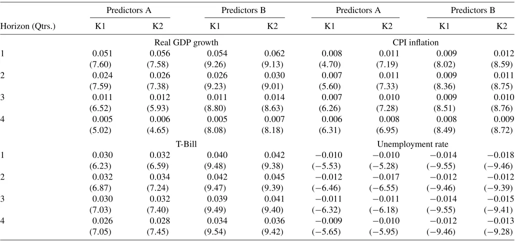
whereϕτh|T denotes the Kalman smoothed estimates of the h -quarter-ahead forecast for any variable being predicted in the SPF,sτ denotes the surprise component of the nonfarm payrolls release,ητ is an error term, and the regression is run only over days on which there is a nonfarm payrolls release. This gives us a sample size of 182; one observation for each monthly non-farm payroll release from 1990Q3 to 2005Q4. The regression gives an estimate of the average effect of a one unit (100,000) positive nonfarm payrolls surprise onϕτh. OLS coefficient es-timates from Equation (13) are given in Table5, along with
t-statistics constructed using heteroscedasticity-robust standard errors. Most entries are highly statistically significant with ei-ther predictors (a) or (b). The estimated coefficients seem to be of a reasonable magnitude. For example, using predictors (a) and model K2, a 100,000 positive nonfarm payrolls surprise (which is approximately a one standard deviation announce-ment surprise) is estimated to raise one-quarter-ahead growth forecasts by 6/100ths of a percentage point and to raise four-quarter-ahead growth forecasts by 1/100th of a percentage point. And the same positive labor market news is estimated to raise four-quarter inflation forecasts by 1/100th of a percent-age points, and to raise four-quarter T-Bill yield forecasts by 3 basis points. These estimated effects are all small, but it seems reasonable that forecasts are not adjusted much in response to a one-standard deviation surprise in employment growth for one
Table 5. Measuring news impact
Predictors A Predictors B Predictors A Predictors B
Horizon (Qtrs.) K1 K2 K1 K2 K1 K2 K1 K2
Real GDP growth CPI inflation
1 0.051 0.056 0.054 0.062 0.008 0.011 0.009 0.012
(7.60) (7.58) (9.26) (9.13) (4.70) (7.19) (8.02) (8.59)
2 0.024 0.026 0.026 0.030 0.007 0.011 0.009 0.011
(7.59) (7.38) (9.23) (9.01) (5.60) (7.33) (8.36) (8.75)
3 0.011 0.012 0.011 0.014 0.007 0.010 0.009 0.010
(6.52) (5.93) (8.80) (8.63) (6.26) (7.28) (8.51) (8.76)
4 0.005 0.006 0.005 0.007 0.006 0.008 0.008 0.009
(5.02) (4.65) (8.08) (8.18) (6.31) (6.95) (8.49) (8.72)
T-Bill Unemployment rate
1 0.030 0.032 0.040 0.042 −0.010 −0.010 −0.014 −0.018
(6.23) (6.59) (9.48) (9.38) (−5.53) (−5.28) (−9.55) (−9.46)
2 0.032 0.034 0.042 0.045 −0.012 −0.017 −0.012 −0.012
(6.87) (7.24) (9.47) (9.39) (−6.46) (−6.55) (−9.46) (−9.39)
3 0.030 0.032 0.039 0.041 −0.011 −0.011 −0.014 −0.015
(7.03) (7.40) (9.49) (9.40) (−6.32) (−6.18) (−9.55) (−9.41)
4 0.026 0.028 0.034 0.036 −0.009 −0.010 −0.012 −0.013
(7.05) (7.45) (9.54) (9.42) (−5.65) (−5.95) (−9.46) (−9.28)
NOTE: The table reports coefficient estimates in regressions of Kalman Smoothed estimates of SPF Forecast revisions on the surprise components of nonfarm payroll announcements. The coefficient estimates are Effects of 100,000 surprise witht-statistics in parentheses.
Ghysels and Wright: Forecasting Professional Forecasters 515
month. And, though small, these effects are all highly signifi-cant.
It is worth mentioning that throughout this exercise, we did not impose any rationality on the expectations. The hypothe-sis of rationality of survey expectations has been examined and tested by many authors, with mixed results. Much of the dis-crepancy appears to relate to the sample period considered (see, for example, Ang, Bekaert, and Wei2007). In the 1970s, the surveys appear to have had poor success in forecasting some variables, especially inflation, but have been more successful subsequently. We are focusing the more recent period in which the surveys have been found to fare better.
5. CONCLUSIONS
Survey forecasts provide useful information about agents’ expectations. However, since they are released infrequently, these surveys are often stale, and it would seem useful to be able to measure respondents’ expectations, and to predict up-coming survey releases, at a higher frequency. We have pro-posed methods for doing so using daily financial market data, and found that the resulting predictions allow researchers to an-ticipate a substantial portion of the revisions to survey forecasts. We have also shown how daily estimates of respondents’ ex-pectations can allow us to measure the effects of events and news announcements on these expectations. MIDAS methods can also be used for forecasting outcomes (as opposed to sur-vey expectations) using daily asset price data. Our results show that this is indeed the case with a degree of success that com-pares favorably with professional survey forecasts. Hence, our relatively simple methods match the often opaque survey meth-ods based on a plethora of information sources.
The article makes clear the value of estimating what profes-sional forecasters would predict if they were asked to forecast daily. The practical application of these techniques promotes the refinement of specifications that in the future will generate models more accurate than those presented in the article.
The methods used in this article can also be applied to indi-vidual forecasts, instead of the median forecast. This would al-low us to further investigate interesting issues about individual forecasts such as most recently discussed in Gallo, Granger, and Jeon (2002). They presented evidence, using data from Consen-sus Forecasts, that views expressed by other forecasters in the previous period influence individuals’ current forecast. With a MIDAS approach we can see how much of the public informa-tion affects individual forecasters, particularly, given their past prediction record. We leave this for future research.
APPENDIX: DERIVATION OF PROJECTION EQUATION
In this appendix we derive Equation (5). We noted that according to Equation (4) the partial sums process Sτ = τ
d=lt−1+1vd behaves like a random walk and, therefore, the
pricepτt behaves like a random walk plus noise. Note that this is a “local behavior” during the quarter fromt−1 to t. Here we will assume a standard random walk plus noise process (as if it applied throughout, not just locally) to derive an approxi-mate prediction formula. To distinguish the model from that in Section2we use, at first different notation, and subsequently
map the results into the setting of Section2. More specifically, we start from the standard random walk plus noise model (see, e.g., Whittle1983and Harvey and De Rossi2006):
˜
pt=μt+ξt,
(A.1) μt=μt−1+ηt,
whereξtandηtare mutually uncorrelated Gaussian white noise
disturbances with variancesσξ2andση2, respectively. Define the signal-to-noise ratio q=ση2/σξ2>0 then the one-sided sig-nal extraction filter for μt given {˜pt−j}∞j=0, denoted μˆt|t has
weights̟j(see Whittle1983and Harvey and De Rossi2006):
ˆ in the sense that it applies to observations “near” t, whereas observations in the remote past have weights of the two-sided filter, namely(1+ζ )(−ζ )j/(1−ζ ). See, e.g., Harvey and De Rossi (2006), equations (2.11), (2.13), and (2.15) for further discussion. One can also derive exact weights for a finite sam-ple, see Whittle (1983, chapter 7). This would involve a lot of cumbersome notation, which we avoid here. From Equa-tion (A.2) we can derive the first-difference version p˜t = r˜t,
As noted, the partial sum processSτ implied by Equation (4) behaves locally like a random walk plus noise. Hence, we can use the above formula as an approximation, treating returns as if they are zero prior to the beginning of the quarter (d <0 in Section 2) and substituting into Equation (3) yields Equa-tion (5). The formula is only an approximaEqua-tion and a more rig-orous formula can be derived, using the finite sample exact fil-ters weights. Deriving such filfil-ters is rather involved, see, e.g., Whittle (1983) and Schleicher (2006), and we do not really need the exact filter weights for motivational purpose.
516 Journal of Business & Economic Statistics, October 2009
ACKNOWLEDGMENTS
The authors thank the Associate Editor, two referees, as well as Andrew Ang, Mike McCracken, Nour Meddahi, Jim Stock, Rossen Valkanov, and Min Wei for helpful comments. All re-maining errors are our own.
[Received August 2006. Revised September 2007.]
REFERENCES
Ang, A., Bekaert, G., and Wei, M. (2007), “Do Macro Variables, Asset Markets or Surveys Forecast Inflation Better?”Journal of Monetary Economics, 54, 1163–1212.
Ang, A., Piazzesi, M., and Wei, M. (2006), “What Does the Yield Curve Tell Us About GDP Growth?”Journal of Econometrics, 131, 359–403. Bernanke, B. S., Gertler, M., and Watson, M. (1997), “Systematic Monetary
Policy and the Effects of Oil Price Shocks,”Brookings Papers on Economic Activity, 1, 91–157.
Breeden, D. T., Gibbons, M. R., and Litzenberger, R. (1989), “Empirical Tests of the Consumption-Oriented CAPM,”Journal of Finance, 44, 231–262. Christoffersen, P., Ghysels, E., and Swanson, N. (2002), “Let’s Get ‘Real’
About Using Economic Data,”Journal of Empirical Finance, 9, 343–360. Croushore, D. (1993), “Introducing: The Survey of Professional
Forecast-ers,” Federal Reserve Bank of Philadelphia Business Review, Novem-ber/December, 3–14.
Gallo, G., Granger, C. V. J., and Jeon, Y. (2002), “Copycats and Common Swings: The Impact of the Use of Forecasts in Information Sets,”IMF Staff Papers, 49, 4–21.
Ghysels, E., and Wright, J. (2006), “Forecasting Professional Forecasters,” Working Paper 2006-10, FEDS, available athttp:// papers.ssrn.com/ sol3/ papers.cfm?abstract_id=885671.
Ghysels, E., Santa-Clara, P., and Valkanov, R. (2005), “There Is a Risk-Return Tradeoff After All,”Journal of Financial Economics, 76, 509–548.
(2006), “Predicting Volatility: Getting the Most Out of Return Data Sampled at Different Frequencies,”Journal of Econometrics, 131, 59–95. Ghysels, E., Sinko, A., and Valkanov, R. (2006), “MIDAS Regressions: Further
Results and New Directions,”Econometric Reviews, 26, 53–90.
Harvey, A. C. (1989),Forecasting, Structural Time Series Models and the Kalman Filter, Cambridge: Cambridge University Press.
Harvey, A. C., and De Rossi, G. (2006), “Signal Extraction,” inPalgrave Hand-book of Econometrics, Vol. 1, eds. K. Patterson and T. C. Mills, Bas-ingstoke, U.K.: Palgrave MacMillan, pp. 970–1000.
Harvey, A. C., and Pierse, R. G. (1984), “Estimating Missing Observations in Economic Time Series,”Journal of the American Statistical Association, 79, 125–131.
Lamont, O. (2001), “Economic Tracking Portfolios,”Journal of Econometrics, 105, 161–184.
Schleicher, C. (2003), “Kolmogorov–Wiener Filters for Finite Time Series,” Discussion Paper 109, Society for Computational Economics.
Stock, J. H., and Watson, M. (1989), “New Indexes of Coincident and Leading Economic Indicators,” inMacroeconomics Annual, Vol. 4, eds. O. Blan-chard and S. Fischer, Cambridge, MA: MIT Press.
(2002), “Macroeconomic Forecasting Using Diffusion Indexes,” Jour-nal of Business and Economic Statistics, 20, 147–162.
(2003), “Forecasting Output and Inflation: The Role of Asset Prices,”
Journal of Economic Literature, 41, 788–829.
Townsend, R. M. (1983), “Forecasting the Forecasts of Others,”Journal of Po-litical Economy, 91, 546–588.
Whittle, P. (1983),Prediction and Regulation(2nd ed.), Minneapolis: Min-nesota University Press.
Zadrozny, P. A. (1990), “Estimating a Multivariate ARMA Model With Mixed-Frequency Data: An Application to Forecasting U.S. GNP at Monthly In-tervals,” working paper, Federal Reserve Bank of Atlanta.