Full Terms & Conditions of access and use can be found at
http://www.tandfonline.com/action/journalInformation?journalCode=ubes20
Download by: [Universitas Maritim Raja Ali Haji] Date: 11 January 2016, At: 19:31
Journal of Business & Economic Statistics
ISSN: 0735-0015 (Print) 1537-2707 (Online) Journal homepage: http://www.tandfonline.com/loi/ubes20
A New Linear Estimator for Gaussian Dynamic
Term Structure Models
Antonio Diez de Los Rios
To cite this article: Antonio Diez de Los Rios (2015) A New Linear Estimator for Gaussian Dynamic Term Structure Models, Journal of Business & Economic Statistics, 33:2, 282-295, DOI: 10.1080/07350015.2014.948176
To link to this article: http://dx.doi.org/10.1080/07350015.2014.948176
View supplementary material
Accepted author version posted online: 08 Aug 2014.
Submit your article to this journal
Article views: 280
View related articles
View Crossmark data
A New Linear Estimator for Gaussian Dynamic
Term Structure Models
Antonio DIEZ DE LOS
RIOS
Financial Markets Department, Bank of Canada, Ottawa, Ontario, K1A 0G9, Canada ([email protected])
This article proposes a novel regression-based approach to the estimation of Gaussian dynamic term structure models. This new estimator is an asymptotic least-square estimator defined by the no-arbitrage conditions upon which these models are built. Further, we note that our estimator remains easy-to-compute and asymptotically efficient in a variety of situations in which other recently proposed approaches might lose their tractability. We provide an empirical application in the context of the Canadian bond market.
KEYWORDS: Affine term structure model; Asymptotic least squares; Bond risk premia; Singular co-variance matrix; Unspanned factors.
1. INTRODUCTION
The maximum likelihood (ML) approach is considered as the most natural way to estimate Gaussian dynamic term structure models (GDTSMs), since they provide a complete characteriza-tion of the joint distribucharacteriza-tion of yields. However, the solucharacteriza-tion of the optimization problem involving maximization of the density of the yields does not exist in closed form, except in very few specific cases. Consequently, researchers often have to rely on cumbersome optimization techniques to estimate the parameters of the model, facing diverse numerical issues that are usually magnified by (i) the large number of parameters describing the dynamics of the term structure of interest rates, (ii) the highly nonlinear nature of the likelihood function, and/or (iii) the ex-istence of multiple local optima (see, e.g., the discussions in Duffee and Stanton2012; Hamilton and Wu2012).
Motivated by these numerical challenges, this article con-siders a new linear regression approach to the estimation of GDTSMs that can completely avoid numerical optimization methods whenever yields on adjacent maturities are directly observed (i.e., whenever the researcher observes yields on both 16-quarter and 17-quarter bonds). Specifically, our linear estimator is an asymptotic least-square (ALS) estimator that exploits three features that characterize this class of models. First, GDTSMs have a reduced-form representation whose parameters can be easily estimated via a set of ordinary least-square (OLS) regressions. Second, the no-arbitrage assumption upon which GDTSMs are built can be characterized as a set of implicit constraints between these reduced-form parameters and the parameters of interest. Third, this set of restrictions is linear in the parameters of interest. Consequently, we propose a two-step estimator. In the first step, estimates of the reduced-form parameters are obtained by OLS. In the second step, the parameters of the GDTSMs are inferred by forcing the no-arbitrage constraints, evaluated at the first-stage estimates of the reduced-form parameters, to be as close as possible to zero in the metric defined by a given weighting matrix. Note that, since the constraints are linear in the parameters of interest, the solution to the estimation problem in this second step is known in closed form. In fact, in its most basic form (i.e., using an iden-tity weighting matrix), the estimates of the parameters of the GDTSMs resemble those obtained from an OLS cross-sectional
regression involving the reduced-form parameter estimates (i.e., the estimated bond factor loadings). Moreover, our ALS estimator is consistent and asymptotically normally distributed. Recent approaches to the estimation of GDTSMs that have substantially lessened some of the numerical challenges faced by researchers include the ML approach of Joslin, Singleton, and Zhu (2011), the minimum-chi-square estimator of Hamilton and Wu (2012), and the regression-based approach of Adrian, Crump, and Moench (2013). We note that the optimal ALS estimator of the parameters of a GDTSM satisfies the condi-tions in Diez de los Rios (2014) under which ALS estimation is asymptotically equivalent to MLE (i.e., the estimator of Joslin, Singleton, and Zhu2011). We also show that both the Hamilton and Wu (2012) and Adrian, Crump, and Moench (2013) esti-mators are ALS estiesti-mators, where these estiesti-mators differ from ours either in the weighting matrix employed, the parameteri-zation of the no-arbitrage conditions, the reduced-form model estimates, and/or the existence of restrictions on the parameters of interest. This unified framework allows us to conclude that our ALS estimator remains tractable and asymptotically effi-cient in a variety of situations in which the other approaches might lose their tractability.
We discuss several extensions of our estimation method in-cluding how to estimate GDTSMs subject to certain equality constraints on the structural parameters (see, e.g., Cochrane and Piazzesi2008), how to estimate GDTSMs where some of the factors are unspanned (see, e.g., Joslin, Priebsch, and Singleton
2014), and how to address some of the biases associated with the extreme persistence found in interest rates (see, e.g., Bauer, Rudebusch, and Wu2012).
For illustrative purposes, we estimate a three-factor model and decompose the Canadian 10 year zero-coupon bond yield into an expectations and term premium component. Our three-factor specification is designed to capture all the economically interest-ing variation in both the cross-section of interest rates and bond
© 2015American Statistical Association Journal of Business & Economic Statistics
April 2015, Vol. 33, No. 2 DOI:10.1080/07350015.2014.948176
Color versions of one or more of the figures in the article can be found online atwww.tandfonline.com/r/jbes.
282
risk premia, and resembles the Cochrane and Piazzesi (2008) model of the U.S. yield curve. Specifically, we identify our first two factors with the first two principal components of the Canadian yield curve, while the third one is a return-forecasting factor similar in spirit to that presented in Cochrane and Piazzesi (2005). Moreover, we exploit the numerical tractability of our estimation method to compute bootstrapp-values that correct for the generated regressor problem inherent in the estimation of our model.
The structure of the article is as follows. In Section2, we briefly describe the class of GDTSMs and introduce our new lin-ear estimator. In Section3, we reinterpret this estimator within the ALS framework. We discuss the relationship between our method and other recently suggested approaches to the esti-mation of GDTSMs in Section 4. Section5 discusses several extensions of our regression-based framework, and Section6
contains our empirical results. Section7 concludes. Auxiliary results, including a Monte Carlo that confirms that the tractabil-ity of the ALS estimator does not come at the expense of ef-ficiency losses or bad finite-sample properties, are gathered in the online Appendix.
2. GAUSSIAN AFFINE TERM STRUCTURE MODELS
2.1 General Framework
We start by considering an (M×1) vector of state variables (or pricing factors), ft, that describes the state of the economy.
For the moment, we remain “agnostic” as to the nature of these pricing factors. The dynamic evolution of the state variables un-der the physical, or historical measure,P, is given by a Gaussian VAR(1) process:
ft+1=µ+ft+vt+1, (1)
wherevt+1∼iidN(0,).
Letrtbe the continuously compounded one-period, or
short-term, interest rate. The short rate is related to the set of state variables through the following affine relation:
rt =δ0+δ′1ft. (2)
The model is completed by specifying the stochastic discount factor (SDF) to be exponentially affine in ft (e.g., Ang and
Piazzesi2003):
itive) SDF,ξt+1, can be used to price zero-coupon bonds using
the following recursive relation:
where Pt,n is the price of a zero-coupon bond of maturity n
periods at timet. In particular, it is possible to show that solving Equation (4) is equivalent to solving the following equation:
Pt,n=E
whereEtQdenotes the expectation under the risk-neutral prob-ability measure,Q. Under the risk-neutral probability measure,
the dynamics of the state vector ft are characterized by the
following VAR(1) process:
Solving (4), we find that the continuously compounded yield on ann-period zero-coupon bond at timet,yt,n= −n1logPt,n,
is given by
yt,n=an+b′nft, (6)
wherean= −An/nandbn= −Bn/n, andAnand Bnsatisfy
the following set of recursive relations:
B′n= B′n−1
sideration. The recursion is started by exploiting the fact that the affine pricing relationship is trivially satisfied for one-period bonds (n=1), which implies thatA1= −δ0,andB1= −δ1.
2.2 A New Linear Estimator for GDTSMs
An important characteristic of the Gaussian affine bond pric-ing model above is that the pricpric-ing recursive relations in (7) and (8) are linear inQ andµQ. Therefore, if the innovation covariance matrixand the set of coefficientsAnandBnwere
observed directly, one could easily estimate the risk-neutral pa-rameters of the model using a set of (cross-sectional) OLS re-gressions. In such a case, the linear structure of the model would allow us to recover an estimate ofQfrom the (cross-sectional) OLS regression of (B′
while an estimate ofµQcan be obtained from the regression of (An−An−1−12B′n−1Bn−1−A1) onB′n−1:
However, this linear estimator is infeasible because the innova-tion covariance matrix, and the set of coefficientsAnandBn
are, in practice, unknown. Nevertheless, consistent estimates of these objects are readily available from a reduced-form repre-sentation of the model (see Hamilton and Wu2012). We pro-pose, instead, to replace the unknown objects in Equations (9) and (10) by consistent estimates obtained from the reduced-form representation of the model.
To obtain the reduced-form representation of the GDTSM, it is convenient to resort to the state-space representation of the ob-served variables (i.e., the bond yields) implied by the model. In a general state-space representation, there is a transition equation that describes the dynamic evolution of the state factors over time, and a measurement equation that relates the observed data
to the state factor. In terms of our asset pricing model, the VAR dynamics in (1) can be interpreted as the transition equation, while the pricing relationship in (6) is the measurement equa-tion. Letyo
t,ndenote the observed yields, which we assume are
subject to measurement error. Let yt =[yt,1, yt,2, . . . , yt,N]′be
the vector of model-implied yields that stack the affine mapping (6), and let yo
t be the equivalent vector of observed yields. Let
ηtbe a zero-mean measurement error that is iid across time and
that has a covariance matrix. Then, the asset pricing model, joint with our assumption on the measurement errors, implies that the vector yo
t has the following state-space representation:
yot =a+bft+ηt, (11)
ft =µ+ft−1+vt, (12)
where a=a(µQ,Q,)
andb=b(Q) are nonlinear func-tions of µQ
, Q
, and . For completeness, we assume that
E(ηtvs)=0for alltands.
Once again, estimation of the reduced-form parameters in Equations (11) and (12) could be greatly simplified if the bond factors, ft, were observed. Specifically, since the errors of the
model are conditionally homoscedastic, the ML estimates of the reduced-form parameters could be trivially obtained via a set of OLS regressions (see Sentana2002; Hamilton and Wu2012): (i) the (cross-sectional) coefficientsaandbcould be estimated from the OLS regression of yo
t on a constant and ft; (ii) the
(time-series) coefficientsµandcould be estimated from the OLS regression of ft on a constant and its lag.
To overcome this issue, we follow Joslin, Singleton, and Zhu (2011) in working with bond state variables that are lin-ear combinations (i.e., portfolios) of the yields themselves, ft = P′yot, where P is a full-rank matrix of weights, and by
further assuming that ft is observed perfectly (alternatively,
we could work with observable factors such as macroeconomic variables). That is, P′(yo
t −yt)=P′ηt =0 ∀t. This
assump-tion allows us to factorize the joint likelihood funcassump-tion into the marginal component of ft and the conditional components
corresponding to all the individual yields. That is, this assump-tion makes ft observable in practice and, as noted above,
al-lows us to obtain ML estimates of the reduced-form param-eters by OLS. We further assume that =σ2η×(P⊥P′⊥), where P′
⊥ is a basis for the orthogonal component of the row span of P′. This guarantees that P′P =0 and al-lows to concentrate σ2η from the likelihood function through
σ2
η =
T t=1
N
n=1(y
o
t,n−yt,n)2/(T ×(N−M)).
We end this section by providing a multistep algorithm that summarizes the implementation of our new linear estimator for GDTSMs:
Step 1. Estimate the parameters of the reduced-form model by linear regressions:
(1a) Estimate the cross-sectional coefficientsaandbin Equation (11) from OLS regressions of the observed yields, yo
t, on a constant and the bond factors ft.
(1b) Obtain the coefficients µ, , and driving the VAR dynamics in (1) by OLS.
Step 2. Recover the coefficients driving the risk-neutral dy-namics of the factors using cross-sectional regressions:
(2a) RecoverAn= −nan and Bn= −nbn, wherean,
andbnare the estimates ofaandbobtained in Step
1. Setδ0=a1andδ1 =b1
(2b) Run the cross-sectional regressions in (9) and (10) to obtain an estimate ofµQandQ.
Step 3. Obtain an estimate of the prices of risk as a differ-ence between the coefficients driving the dynamics under the physical and risk-neutral measures:λ0=µ−µQand λ1=−
Q .
3. ASYMPTOTIC LEAST-SQUARE ESTIMATION OF GDTSMS
3.1 The Asymptotic Least-Square Estimation Framework
In this section, we provide an alternative interpretation of the linear estimator described above based on the ALS framework of Gourieroux, Monfort, and Trognon (1982,1985) (GMT here-after). As noted by these authors, many empirical models can be formalized as a set of relationshipsg(π, θ)=0between the parameters of interestθ, and a set of auxiliary parametersπ. In the case of the estimation of GDTSMs, we advance thatθ is related to the parameters of the no-arbitrage model in Equa-tions (1), (2), and (5); π is related to the set of parameters from the reduced-form model in Equations (11) and (12); the set equationsg(π, θ)=0is related to the pricing recursions in equations and (7) and (8); andg(π, θ) is linear inθ.
To be more specific, we assume that the set ofGimplicit equa-tionsg(π, θ)=0has a unique solution forθ∈⊂RK given
π∈⊂RH. This guarantees that the parameters of interest
can be determined without ambiguity from the auxiliary param-eters. Further, we assume the existence of a strongly consistent and asymptotically normal estimator of the auxiliary parame-tersπ, such that asT → ∞,π →π0,P
θ0 almost surely; and √
T(π−π0)−→d N[0,Vπ(θ0)],whereTdenotes the number
of observations in the sample and θ0 and π0 denote the true value of the parameters of interest and auxiliary parameters, respectively, that is,g(π0,θ0)=0
.
The ALS estimation principle consists of minimizing a quadratic form in the distance function evaluated at the esti-mates of the auxiliary parameters,π:
θALS=arg min
θ Tg(π,θ) ′W
Tg(π,θ), (13)
whereWTis a positive semidefinite weighting matrix that
possi-bly depends on the observations. In other words, GMT proposed forcing theGimplicit equations evaluated atπ to be as close as possible to zero in the metric defined byWT. Further notice
that, when the distance function is linear in the set of parameters of interest (as in the case of the estimation of GDTSMs), the solution to the optimization problem in (13) is known in closed form.
Further, assuming thatg(π, θ)is twice continuously differen-tiable;WT convergesPθ0 almost surely toW,a nonstochastic
semidefinite weighting matrix of sizeG,and rank greater or equal thanK; the true values of the parameters of interest and auxiliary parameters,θ0 andπ0, both belong to the interior of
and, respectively; and ∂∂gθ′W∂∂θg′ evaluated at θ0 andπ0 is nonsingular (which implies that the rank of∂g/∂θ′=Kand thatK≤G); then (see GMT for the proof)θALSis strongly
con-sistent for every choice ofWT,and its asymptotic distribution
is given by
where the various matrices in this equation are evaluated atθ0
andπ0.
3.2 The Case of GDTSMs
In the specific example of GDTSM, we have that the vec-tor of auxiliary parameters is given byπ =(π′
1,π′2,π′3)′(i.e.,
the reduced-form parameters), whereπ1 =vec[(a b)′], π2 =
vec[(µ )′],andπ3 = vech(1/2)′.To guarantee the positivity of the covariance matrix, we focus on its Cholesky decompo-sition,=1/21/2′rather than onitself. Thus, we have a total ofH=(N+M)×(M+1)+M×(M+1)/2 auxiliary parameters.
Note that the ML estimation of the reduced-form parameters coincides with OLS estimation equation-by-equation, and there-fore there is a consistent and asymptotically normal estimateπ available. Specifically, we have that
√
Next, we consider the pricing recursions in Equations (7) and (8). By stacking these two sets of equations for all bond yields, we can express the restrictions implied by the no-arbitrage model in compact form as
G(π, θ)′=Y(π)−X(π)Q′=0, (16)
and whereQis a matrix that collects the parameters driving the dynamics under the risk-neutral measure:
Q′=
In addition to considering vec(Q), it is convenient to add the parameters describing the dynamics of the factors under the physical measure to the vector of structural parameters,θ, such thatθ =(θ′1,θ′
2,θ′3)′, whereθ1=vec(Q),θ2=vec[(µ )′],
andθ3=vech(1/2). Thus, we have a total ofK=(2M+1)×
(M+1)+M×(M+1)/2 parameters of interest.
By vectorizing Equation (16) and adding the set of identities θ2=π2andθ3=π3, we arrive at the following expression for the number of distance functions is equal to the number of auxiliary parameters, that is,G=H.
We note that the linear estimator proposed in Section2.2is nu-merically equivalent to the estimator that minimizes a quadratic form in the distance function, evaluated at the estimates of the reduced-form parameters, π, where the weighting matrix has been chosen to be the identity matrix,WT = I:
θOLScan be obtained by specializing Equation (14) to the case
ofW =Iand∂g/∂θ′= −Ŵ(π0).
3.3 Self-Consistency
As noted by Cochrane and Piazzesi (2005), one should guar-antee that, when choosing state variables that are linear combi-nations (portfolios) of the yields, ft =P′yot, the state variables
that come out of the model need to be the same as the state variables that we started with. In other words, it is necessary to ensure that the pricing of portfolios of yields is also consistent with Equation (6) such that ft = P′yt= P′a(θ)+P′b(θ)ft.
Thus, self-consistency of the model amounts to imposing the following set of constraints when estimating the model:
P′a(θ)=0, P′b(θ)= I. (20)
Let r(θ)=0 denote the set of S=M×(M+1) self-consistency restrictions implicit in Equation (20).
While the OLS estimator in Equation (18) does not satisfy these constraints, we find that, in practice,θOLSdelivers
param-eter estimates that almost satisfy such restrictions. Two features of our proposed estimation approach explain this result. First, given our assumption that ft is observed perfectly, the OLS
estimates of the reduced-form coefficients automatically satisfy such restrictions:
P′a=0, P′b=I, (21)
and, second, our linear estimator tries to match those as closely as possible. In fact, sinceθOLS converges to the true value of
the parameter of interestθ0andr(θ0)=0, we can think of the OLS estimator in Equation (18) as imposing the self-consistency conditions asymptotically.
3.4 Optimal Asymptotic Least Squares of GDTSMs
As in the case of generalized method of moments (GMM) estimation, an identity weighting matrix is not necessarily optimal and (asymptotic) efficiency gains can be achieved by selecting an appropriate weighting matrix. In particular, GMT showed that when ∂π∂g′Vπ are nonsingular when evaluated at θ0 and π0 (which implies
that the rank of ∂g/∂π′=G and that G≤H), then an optimal estimator exists in the sense that the difference between the asymptotic variance of the resulting ALS estimator and another ALS estimator based on any other quadratic form in the same distance function is negative semidefi-nite. In particular the optimal ALS estimator corresponds to the choice of a weighting matrix WT that converges to
W =(∂g
∂π′Vπ ∂g′ ∂π)−
1. Note that, by the delta method, we have that
Vg(θ0)=avar[ so the optimal weighting matrix is simply the inverse of the asymptotic covariance of the distance function evaluated at the estimates of the auxiliary parameters. Similarly, given that r(θ0)=0, one would expect efficiency gains by imposing the self-consistency restrictions in (20) when estimating the param-eters of interest. Therefore, optimal ALS estimation should, in principle, involve both choosing an optimal weighting matrix and simultaneously imposing the self-consistency constraints when estimating the model.
However, as noted in Section2.2, the self-consistency restric-tions combined with the assumption that the bond state variables are observed perfectly imply that, the covariance of the mea-surement errors in Equation (11) is singular. In particular, note thatappears in the expression of the asymptotic covariance matrix of the estimator ofπ1in Equation (15). Thus, the reduced
rank structure intranslates into a reduced-rank structure in Vπ. Further, given that∂g/∂π′is a nonsingularH×Hmatrix,
the singularity inVπalso carries over toVg.
To overcome this problem, we follow Pe˜naranda and Sentana (2012), who studied the problem of obtaining an optimal GMM estimator when the asymptotic variance of the moment condi-tions is singular in the population. Specifically, we (i) replace the ordinary inverse ofVg(θ0), which cannot be defined when
S >0,by any of its generalized inversesV+g(θ0) and, (ii)
simul-taneously, impose the self-consistency restrictions in Equation (20) when estimating the model.
To provide intuition on the optimality of this approach (see Diez de los Rios2014for a formal proof), let the spectral de-composition ofVg(θ0) be written as trix. Therefore, we can split our set of distance functions into two groups: (i) the set ofK−Sdistance functionsT′
1g(π,θ)
whose asymptotic long-run variance is the nonsingular matrix , and (ii) the set of degenerateSdistance functionsT′
2g(π,θ)
that converge in mean square to zero because the set of param-eters of interest satisfy the self-consistent restrictionsr(θ)=0. Focus now, for convenience and without loss of generality, on the Moore–Penrose generalized inverse ofVg(θ0), such that
VMP+
g (θ
0
)=T1−1T′1.
Then, the optimal ALS estimator in this singular setup is equiv-alent to the constrained ALS estimator that works with the re-duced set ofK−S distance functions T′
1g(π,θ)and the
re-strictions r(θ)=0. In this way, note that the ALS estimator that uses the generalized inverse of Vg(θ0) alone without the
self-consistency restrictions will not likely be optimal, since it drops theSasymptotically degenerate, that is, most informative, linear combinations of√Tg(π,θ).
Consequently, we have that the optimal estimator of the pa-rameters of interest is strained generalized least-square (CGLS) estimator. The asymp-totic distribution of this estimator is given by (see chap. 10 in Gourieroux and Monfort1995)
√
π0. Further, as in the case of GMM, the optimized value of
the ALS criterion function has an asymptotic χ2 distribution
with degrees of freedom equal to the number of overidentifying restrictions (G−K).
Unfortunately, the solution to the optimal ALS (i.e., the CGLS) estimator in Equation (22) is not known in closed form becauser(θ) is not linear in the set of parameters of interest,θ. Still, as noted by Newey and McFadden (1994) and Gourieroux and Monfort (1995) among others, estimating the model subject to a linearized version of the constraint delivers an estimator that is asymptotically equivalent to the one that uses the non-linear constraint. For this reason, we start by considering the (suboptimal) ALS estimator that uses a consistent estimate of
the generalized inverse ofVg(θ) as weighting matrix but that
does not impose the restrictionsr(θ)=0:
θGLS=
Ŵ′V+gŴ
−1 Ŵ′V+gγ
. (24)
We will refer to this estimator as the generalized least-square (GLS) estimator. Then, the linearized constrained GLS estima-tor,θCGLSis defined as
θCGLS=arg min
θ T
γ−Ŵθ′V+g γ−Ŵθ
s.t.r(θGLS)=
∂r(θGLS)
∂θ′ (θGLS−θ), (25)
where the constraint r(θ)=0 has been linearized around the unconstrained (GLS) estimate of θ,θGLS. The main
advan-tage of such linearization is that, since the objective function is quadratic and the restrictions are now linear in the parameters of interest, the solution of the estimation problem is known in closed form:
θCGLS=θGLS−J−
1∂r(θGLS)′
∂θ
×
∂r(θGLS)
∂θ′ J
−1∂r(θGLS)′
∂θ −1
r(θGLS), (26)
whereJ =(Ŵ′V+gŴ). However,θCGLSstill does not satisfy the
constraintr(θ)=0exactly, even thoughθCGLSis asymptotically
equivalent to the estimator that uses the nonlinear constraint. This is why we follow Bekaert and Hodrick (2001) in iterat-ing Equation (26) when constructing our constrained estimates. Specifically, we start by obtaining a first restricted estimate of θ using Equation (26) and linearizing the constraint r(θ)=0
aroundθGLS. Denote this first restricted estimateθ (1)
CGLS. Then,
we substitute the initial unconstrained estimate,θGLS, in (26) θ(1)CGLSto obtain a second restricted estimate ofθ. Denote this second restricted estimate byθ(2)CGLS. We repeat this process until the resulting constrained estimate satisfies the self-consistency restrictions,r(θ(CGLSn) )=0within a given tolerance. In practice, only a few iterations of Equation (26) are required.
We note that the CGLS estimates of the coefficients driving the conditional mean of the pricing factors under the physical measure,θ2=vec[(µ )′]′, coincide with the OLS estimates
of the VAR(1) process in (1). On the other hand, the estimate of θ3=vech(1/2)′gets updated given that the CGLS estimates
incorporate the information about contained in the cross-section of interest rates.
Finally, one has to be careful not to delete any of the iden-tity equations ing(π,θ)=0that defineθ2 =π2andθ3=π3
when computing the generalized inverse of Vg. In particular,
g1(π, θ) = vec[G(π, θ)] with G(π, θ)in Equation (16) does
not identifyθ2, and only weakly identifiesθ3 (i.e., the
innova-tion parameters of the VAR dynamics underPonly appear in the pricing equations through a (small) Jensen’s inequality term). Thus, eliminating any of the identities in g2(π, θ)=π2−θ2
org3(π, θ)=π3−θ3, might lead to numerical instabilities of
the CGLS estimates. Appendix A provides a way to compute the generalized inverse ofVgthat avoids this problem.
3.5 Relationship With Maximum Likelihood Estimation
In the standard case, Kodde, Palm, and Pfann (1990) pre-sented the conditions under which the optimal ALS estimator is equivalent to the ML estimator. In particular, these authors noted that if (i) the system of relationships g(π, θ)=0is complete, that is,G=H and the Jacobian∂g/∂θ′has full rank; and (ii) πis estimated by ML, or a method asymptotically equivalent to ML, then the optimal ALS estimator is asymptotically equiva-lent to the ML estimator ofθ. The intuition behind this result lies in the fact that, when g(π, θ)=0 is complete, we have that∂π/∂θ′= −(∂g/∂π′)−1(∂g/∂θ′) as a result of the implicit function theorem.
Diez de los Rios (2014) extended the results in Kodde, Palm, and Pfann (1990) to the case of optimal ALS estimation in a singular setup. In such a case, the optimal ALS estimator is still asymptotically equivalent to the ML estimator as long as
π is estimated by a method that is asymptotically equivalent to constrained ML (i.e.,πsatisfies the self-consistency restrictions r(θ)=0). We note that the CGLS estimator satisfies these two conditions, and, therefore, it is equivalent to the ML estimator.
4. DISCUSSION OF RELATED LITERATURE
In this section, we compare our linear regression estimator to three recent approaches to the estimation of GDTSMs: the ML approach of Joslin, Singleton, and Zhu (2011), the minimum-chi-squared estimator of Hamilton and Wu (2012), and the regression-based approach of Adrian, Crump, and Moench (2013).
4.1 Joslin, Singleton, and Zhu (2011)
In a recent article, Joslin, Singleton, and Zhu (2011) (JSZ) proposed a new canonical representation of GDTSMs that has substantially lessened many of these numerical challenges faced when estimating GDTSMs by ML. They noted that by focusing on “bond” state variables that are linear combinations (i.e., port-folios) of the yields themselves, it is possible to represent the model in a way such that there is a separation between the pa-rameters driving the state variables under the physical measure,
P,and those in the risk-neutral distribution,Q. Such separation can be exploited to simplify the estimation of the model. In par-ticular, JSZ showed that, under the assumption of stationarity underQ,the generic representation of a GDTSM in Equations (1), (2), and (5) is observationally equivalent to a canonical model withrt=r∞Q +1′Kzt,
zt+1=Qzt+u
Q
t+1,
where the state variablesztare latent,uQt ∼iidN(0,z),1Kis
aK-dimensional vector of ones, the matrixQis in ordered real Jordan form with relevant elements (i.e., eigenvalues) collected in the vectorψ, andztfollows an unrestricted VAR(1) process
under the historical measure,P.
By further realizing that ft= P′yt =P′(az+bzzt),where
az,bzare the constant and factor loadings implied by the JSZ
canonical model bond pricing, and using results on invariant transformations of affine term structure models (see Dai and Singleton2000), JSZ showed that a self-consistent model that
uses state variables that are linear combinations of yields, ft =
P′yt, must satisfy
δ0 =r∞Q −δ′c, δ′=1′KD−1, (27)
µQ =(I−Q)c, Q=DQD−1 ,
where c= P′az, and D=P′bz. As a result, the risk-neutral
dynamics of the yield curve (and therefore, the cross-section of interest rates) is entirely determined by (a)rQ
∞, the long-run mean of the short rate underQ; (b)ψ, the speed of mean rever-sion of the state variables underQ; and (c), the covariance matrix of the innovations from the VAR. On the other hand, the VAR dynamics underPremain unrestricted.
Given this separation between risk-neutral and physical dy-namics, and given the fact that the VAR dynamics remain unre-stricted, JSZ proposed the following two-step estimator. In the first step, they estimatedµandby OLS given that, since the VAR dynamics are unrestricted, OLS recovers the estimates of the conditional mean (Zellner 1962). In the second step, they estimated the remaining parameters of the model (rQ
∞,ψ,) via numerical maximization of the likelihood function taking as given the P-dynamics estimates obtained in the first step. Consequently, JSZ reported improved convergence and speed of ML estimation over other canonical representations.
We can still recover the coefficients of the JSZ canonical representation,
ϕ=r∞Q, ψ′′,vec(µ )′′,vech1/2′′, (28) using our linear estimation framework. To do so, one would start by estimating the model by either OLS or, preferably, CGLS. Second, note from Equation (27) thatQis related to the Jor-dan decomposition of Q. Therefore, an estimate ofQ can be obtained by finding the real Jordan normal form of Q.
In particular, when the eigenvalues in Q are real and dis-tinct,ψQcan be obtained by a simple spectral decomposition of
Q=Ddiag(ψQ)D−1. Third, an estimate of the long-run mean of the short rate underQcan be obtained fromr∞Q =δ0+δ′(I−
Q)−1µQ. Fourth, given the structure of the optimization prob-lems in (18) and (25), the estimates of theP-dynamics parame-ters of the state variables implied by our linear framework also coincide with the OLS estimates of the VAR model in Equation (1). Finally, standard errors for the coefficients of the JSZ canon-ical representation can be obtained using the Delta method and the results in Magnus (1985) regarding differentiation of eigen-values and eigenvectors.
We see two main advantages of our linear regression ap-proach when compared to JSZ. First, while avoiding numerical optimization, the estimates of the JSZ normalization param-eters obtained from the self-consistent GLS estimates of the risk-neutral dynamics of the bond factors are asymptotically equivalent to those obtained using the JSZ ML approach (see Section3.5).
Second, we note that by imposing the self-consistency re-strictions using Equation (27) and focusing on their canonical representation of a GDTSM, JSZ were effectively reparameter-izing the model in terms ofK−Sfree parameters (see Propo-sition 1 in Hamilton and Wu2014, for a similar remark). Yet, their normalization requires the analysis of several different
sub-cases depending on whether all the eigenvaluesQare real and distinct, there are repeated eigenvalues or such eigenvalues are complex. In fact, most researchers only analyze the case of real and distinct eigenvalues (e.g., Duffee 2011; Bauer, Rudebusch, and Wu 2012; Joslin, Priebsch, and Singleton 2014). On the other hand, one does not need to a priori determine whether the eigenvalues are real and distinct when estimating the model using our linear regression approach given that our method will, in practice, numerically determine which subcase is most em-pirically relevant.
4.2 Hamilton and Wu (2012)
An alternative estimation method to ML estimation is the minimum-chi-squared estimation proposed by Hamilton and Wu (2012) (HW). These authors proposed to minimize the value of a Wald test statistic for the null hypothesis that the restric-tions implied by the no-arbitrage model are consistent with the data. That is, they proposed to minimize a quadratic form in the difference between the estimated reduced-form parameters and the reduced-form coefficients implied by the no-arbitrage model:
ϕHW=arg min
ϕ T [πHW−pHW(ϕ)] ′V−1
πHW[πHW−pHW(ϕ)],
(29) whereϕis the vector of canonical parameters in Equation (28), and where the reduced-form and implied coefficients,πHWand
pHW(ϕ), respectively, have the subscript HW as a reminder that
the set of reduced-form estimatesπHW used in this estimation
method are not necessarily the same as the ones employed when computing the linear estimator discussed in Section2.2. For ex-ample, the set of bonds used when estimating the model using the HW approach does not need to be the same as the set em-ployed when using our regression-based methods (we return to this point below).
It is thus straightforward to realize that the HW minimum-chi-squared estimator falls within the ALS framework as well. In their case, the distance function is linear in the set of reduced-form coefficients, and the optimal weighting matrix is given by the inverse of the variance of the reduced-form parameters which, ifπHWis estimated by ML, coincides with the
(reduced-form) information matrix. We note that, in fact,πHW can be
viewed as a reparameterization ofπabove in terms ofG−Sfree reduced-form coefficients after imposing the self-consistency restrictions. Consequently, VπHW is, in general, invertible and ϕHW thus optimal. Further, HW showed that their estimation approach is asymptotically equivalent to ML estimation ofϕ, which is a consequence of satisfying the Kodde, Palm, and Pfann (1990) conditions under which an ALS estimator is asymptoti-cally equivalent to the ML estimator.
We note that the CGLS estimator in Equation (25) can also be interpreted as minimizing the value of a Wald test statis-tic for the null hypothesis that the restrictions implied by the no-arbitrage model are consistent with the data (within the set of θ’s that imply a self-consistent model). In particular, the criterion function of our optimal linear estimator resembles a Wald statis-tic for the null hypothesis that g(π,θ)=γ(π)−Ŵ(π)θ=0, which is, in fact, a reparameterization of the null hypothesis considered in HW. Still, it is worth pointing out, again, that
the main advantage of our parameterization is that the distance function is linear inθand, thus, the solution to the minimization of the chi-square criterion function can be obtained in closed form.
The advantages of our method with respect to the HW ap-proach are similar to the advantages with respect to the ML estimator described in the previous section. Moreover, most of the numerical advantages of the HW approach with respect to direct maximization of the likelihood of the model come from considering exactly identified models (i.e., models where the number of linear combinations of yields used in the estimation is equal to N =M+1). That is, one has to discard a lot of information contained in the term structure of interest rates and thus, by reducing the number of bonds used in the estimation of the model, it is possible to incur potentially large efficiency losses.
4.3 Adrian, Crump, and Moench (2013)
In a recent article, Adrian, Crump, and Moench (2013) (ACM) proposed a regression-based approach to the estima-tion of GDTSMs that, as with our ALS approach, completely avoids numerical optimization whenever yields on adjacent ma-turities are directly observed. Using observable pricing factors (i.e., principal components of yields), and focusing on bond excess holding period returns, they developed a four-step OLS estimation method. In their first step, they estimated the VAR(1) process in Equation (1) to obtainµ,, and, and decomposed pricing factors into predictable components and innovations. In the second step, they estimated the exposures of bond returns to (a) lagged levels of pricing factors ft−1, and (b)
contem-poraneous pricing factor innovationsvt. In the third step, they
estimated the market prices of risk parameters,λ0andλ1, from
a cross-sectional regression of exposures to contemporaneous pricing factors (i.e., a la Fama-MacBeth). Finally, they recov-ered parameters of the short rate,δ0 andδ1, by regressing the
short rate on the pricing factors.
We note that the ACM differs from our method (and JSZ and HW for that matter) in the distributional assumption of the pricing errors. In particular, ACM assumed uncorrelated pricing errors on excess returns, instead of uncorrelated pricing errors on the yields. As shown in their article, when yield pricing errors are uncorrelated, the model has the undesirable feature of generating return pricing errors that are cross-sectionally and serially correlated, thus implying the existence of bond return predictability that is not captured by the pricing factors. While (for space considerations and given that the assumption of uncorrelated pricing errors on excess returns is not standard in the literature) we do not explore the ACM assumption on the pricing errors in this article. We note that it is possible to handle autocorrelated yield errors within our framework given that OLS estimates of the reduced-form parameters remain consistent and asymptotically normal under such an assumption.
More importantly, we show in Appendix B how to reinter-pret the ACM estimator within the ALS framework, thus easing the comparison with our proposed linear estimators. By doing so, we find three main advantages of our linear regression ap-proach with respect to ACM. First, we show how to impose self-consistency of the model and how to obtain the parameters of
the JSZ normalization (features absent in the ACM framework). Second, our regression approach is likely to provide asymptotic efficiency gains with respect to ACM, given that they used an identity weighting matrix and did not impose self-consistency of the model. Finally, we show in the appendix that the sys-tem of implicit relationships that defines the ACM estimator is not complete (the number of reduced-form parameters is larger than the dimension of the distance function). Thus, the ACM estimator does not satisfy the conditions under which an ALS estimator is asymptotically equivalent to ML estimation, even if the self-consistency restrictions were imposed and an optimal weighting matrix was chosen.
5. EXTENSIONS
In this section, we present several extensions of our estimation method. Further results related to the estimation of GDTSMs with lags, measurement errors, autocorrelation of the residuals, and temporal aggregation can be found in Appendix C.
5.1 Estimation Subject to Equality Constraints
Several recent studies in this literature have considered esti-mation of GDTSMs subject to certain equality constraints on the structural parameters, including the case where some of the elements of the prices of risk are set to zero (see, e.g., Cochrane and Piazzesi 2008; Bauer 2014; Bauer and Diez de los Rios
2012; Joslin, Priebsch, and Singleton 2014).
A reason for restricting the prices of risk concerns the es-timated persistence of the data. When the prices of risk are completely unrestricted, the largest eigenvalue of the physical measureestimated from the VAR(1) representation in Equa-tion (1) is usually less than 1.00, with the result that expected future bond yields beyond 10 years are almost constant (see, e.g., Bauer, Rudebusch, and Wu 2012). However, the existence of a level factor in the cross-section of interest rates implies a very persistent process for bond yields under the risk-neutral measure. The largest eigenvalue ofQthus tends to be close to or equal to one. By imposing restrictions on the prices of risk, we will be effectively pulling the largest eigenvalue ofcloser to that ofQso that the physical time-series can inherit more of the high persistence that exists under the risk-neutral measure. In fact, motivated by this persistence issue, Joslin, Priebsch, and Singleton (in press) directly forced the largest eigenvalue of to be equal to the largest eigenvalue ofQ.
By having already discussed how to estimate GDTSMs sub-ject to self-consistency restrictions, it is straightforward to see that estimation subject to (additional) equality constraints can naturally be handled in our setup. In the case of optimal ALS estimation, for example, one just needs to (i) add a new set of restrictions to the estimation problem in (25) and (ii) use the iterative procedure described in Section3.4.
5.2 Unspanned Risks
An important development in this literature is the role of unspanned variables (see, e.g., Joslin, Priebsch, and Single-ton 2014). A variable is unspanned if its value is not related to the contemporaneous cross-section of interest rates but it
does help forecast both future excess returns on the bonds (i.e., term structure risk premia) and future interest rates. That is, a variable is unspanned if its bond yield factor loadings are equal to zero, yet it helps in explaining the dynamics of interest rates.
Such unspanned variables can be accommodated in our framework in the following way. Specifically, let the pricing factors ft=(f′1t, f′2t)′ be partitioned into spanned factors
(f1t) and unspanned factors (f2t), and letδ,µQ, andQ be
partitioned accordingly. If (i) the short rates in each country are affine functions of f1t only (δ2=0) and (ii) we set the
right, upper block of the autocorrelation matrix Q to zero (Q12=0), then f2t will be unspanned by the cross-section of
interest rates. Absent these two assumptions, no-arbitrage pric-ing would imply that bond yields would be affine functions of all ft (see Equation (7)). While the no-spanning
assump-tions imply that it is not possible to identifyµQ2,Q21 norQ22,
given that they affect neither the prices of the bonds nor their risk premia (see JPS for additional details), the linear estima-tor in Section2.2(as well as its optimal implementation) can still be easily adapted to recover estimates ofδ1,µQ1, andQ11 from the coefficients of a cross-sectional regression of yields on
f1t.
Our estimation method reveals, however, that caution should be exercised when selecting the factors that explain the cross-section of interest rates. As noted in Section3.1, inference is based on the assumption that∂g/∂θ′has a full-rank structure when evaluated at (π0, θ0). If we wrongly assume that a
fac-tor is spanned when, in fact, it is not, we have that the es-timates of its factor loadings converge to a vector of zeroes. Consequently, rank[∂g/∂θ′]< K and the asymptotic approx-imations to the distribution of the ALS estimator (both OLS and CGLS-type implementation) become nonstandard. In fact, standard inference still breaks down when the b’s are close to zero, that is, ∂g/∂θ′ is almost of reduced rank (see, e.g., Magnusson and Mavroeidis2010). This can occur, for exam-ple, when there are “hidden” factors in the sense of Duffee (2011): the factorj’s loadings are in the neighborhood of zero, so their tiny contemporaneous effect on yields can be lost in the noise that contaminates observed yields. Further, since (the optimal implementation of) our method delivers an estimator that is equivalent to the ML estimator, we suspect that ML estimates of the parameters of the GDTSM might also be sub-ject to weak identification concerns. This situation mirrors the problems that plague the statistical inference in linear factor models when the betas are close to or equal to zero, or the ma-trix of betas has a near-reduced rank (see Kan and Zhang1999; Kleibergen2009; Beaulieu, Dufour, and Khalaf2013). More-over, since the likelihood of weakly identified models tends to exhibit very low curvature with respect to some of the parameters of interest, this might also explain some of the numerical chal-lenges faced by researchers when estimating GDTSMs by ML methods.
5.3 Interpolating Zero-Coupon Bond Yields
While our estimation procedure requires the availability of zero-coupon yields of adjacent maturities, there are some prac-tical situations where only a subset of zero-coupon bond yields
is readily available. In such cases, one could still interpolate the bonds yields of the remaining set of maturities using, for example, spline methods. However, by doing so, one might be introducing (additional) noise from the interpolation of the zero-coupon yield curve into the estimation of the term structure model.
To deal with such situations, we propose to suitably model , that is, the covariance matrix of the measurement errorsηt
in Equation (11), such that the interpolated yields are subject to larger measurement errors than the set of original yields. By following this approach, the efficient ALS estimator will automatically put less weight on the interpolated bonds. In par-ticular, let y1t be the original set of N1 bond yields that are
readily observable, and let H1 be anN1×N selector matrix
of one and zeroes such that y1t =H1yt, where ytis the vector
containing the full set of consecutive maturities fromn=1 to
N.Let y2t =H2yt be the set ofN2=N−N1 (interpolated)
bond yields, whereH2be anN2×Nselector matrix such that
H′
1H2=0(which implies that there is no overlap between the
bonds in the first and second group). Finally, further assume that the bond state variables are linear combinations of the original set of yields only, ft =P′1y
o
1t =P′1H1yt, so that the full-rank
matrix of weights P= P′
1H1.
Specifically, we propose to model the covariance matrix such that (i)1=H1H′1=σ
2
η1×(P1⊥P
′
1⊥), where P′1⊥is a basis for the orthogonal component of the row span ofP′
1,(ii)
2= H2H′2 =σ 2
η2×I, where σ 2
η2/σ 2
η1=ω >1, and (iii)
H1H′2=0. Note that, by appropriately choosing the
parame-terω,a researcher can control how much noisier the interpolated set of bond yields are thought to be when compared to the origi-nal set. We provide an illustration of this approach in Appendix D.
Along these lines, it is important to note that zero-coupon bond yields are not observed in practice and that, instead, re-searchers and practitioners estimate them from price data on Treasury coupon bonds with time-varying maturities (see, e.g., Fama and Bliss1987; Nelson and Siegel1987; Svensson1994). Therefore, one could try to embed the estimation of the zero-coupon bond yield curve into the ALS framework so that automatically reflects the uncertainty regarding the interpola-tion of the zero-coupon yields. Unfortunately, such an approach falls beyond the scope of this article and it is left for further research.
5.4 Small-Sample Standard Errors and Bias Corrections
Given the computational simplicity of our new linear estima-tion method, (small-sample) standard errors can be computed using a parametric bootstrap similar to those in JSZ and Hamil-ton and Wu (2012). The proposed method is as follows:
Step 1. Initialize the artificial samplejof bond factors at their value on the first date from the original sample: f(1j) =
P′yo
1. Consistent with the modelling approach of JSZ, one
needs to assume that the matrix of “portfolio weights,”P, is known and, therefore, remains fixed across bootstrap replications.
Step 2. Generate a sequence{v(tj)}tT=2of N(0,) variables,
and then recursively generate a path of the bond factors f(tj)=µ+f
(j)
t−1+v (j)
t fort =2, . . . , T.
Step 3. Generate a sequence of {η(tj)}tT=1of N(0,)
vari-ables, and then generate a path of the term structure for the original sample size, T, as y(tj) =a(µQ,
Q
,)+
b(Q)f(tj)+η
(j)
t fort =1, . . . , T.
Step 4. Compute an estimate ofθ for the artificial samplej using the linear method described above.
These four steps are repeatedJtimes and small-sample stan-dard errors for the parameters of the model can be computed as the standard deviation of the artificial sequence of bootstrap parameter estimates.
Additionally, since the bond factors are linear combinations of yields, the OLS estimates of the VAR dynamics are likely to be subject to the small-sample biases associated with the extreme persistence found in interest rates (see, e.g., Bekaert, Hodrick, and Marshall1997; Bauer, Rudebusch, and Wu2012). Such a problem can be easily dealt with by adapting Step 2 of our bootstrap. For example, one could correct these OLS estimates using the analytical formula of Pope (1990), using the bootstrap-after-bootstrap method of Kilian (1998), or using the indirect inference estimator of Bauer, Rudebusch, and Wu (2012).
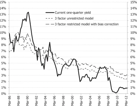
6. DECOMPOSING CANADIAN YIELDS
In this section, we use the iterative procedure outlined in Section3.4to estimate a three-factor model and decompose the Canadian 10-year zero-coupon bond yield into an expectations and term premium component. This three-factor specification is designed to capture all the economically interesting variation in both the cross-section of interest rates and bond risk premia, and resembles the Cochrane and Piazzesi (2008) model of the U.S. yield curve.
Our dataset consists of end-of-quarter observations over the period March 1986 (1986Q1) to June 2012 (2012Q2) of the term structure of Canadian zero-coupon bond yields obtained from the Bank of Canada website. We consider the full spectrum of consecutive maturities from one quarter to 15 years. By focusing on the Canadian bond market, we expect to alleviate some data-snooping concerns related to the fact that most of the research on yield curve modeling and bond premia focuses on U.S. data. To capture the cross-sectional variation of bond yields, we identify our first two factors with the first two principal com-ponents (i.e., level and slope) of the term structure of Canadian interest rates. These two factors explain 99.8% of the varia-tion of yields, and have the tradivaria-tional interpretavaria-tion of level and slope (Litterman and Scheinkman1991). Curvature (i.e., the third principal component) explains only 0.15% of the vari-ability on bond yields. Thus, motivated by parsimony and the discussion on weak identification in Section5.2, we drop the curvature from our study.
Our third factor, on the other hand, builds on the recent evidence documenting the existence of unspanned or nearly spanned factors that are not related to the contemporaneous cross-section of interest rates, but that do help forecast both
fu-ture bond excess returns (i.e., term strucfu-ture risk premia) and future interest rates (see Cochrane and Piazzesi 2008; Duffee
2011). In particular, we include a return-forecasting factor that is similar in spirit to the one presented in Cochrane and Piazzesi (2005), and that captures all of the economically interesting variation in 1 year excess returns for Canadian bonds of all ma-turities. While this factor can be written as a linear combination of yields and it is fully spanned by bond yields, we find that it has very little (if any) explanatory power for the cross-section of interest rates once level and slope are included in the set of fac-tors. Thus, motivated by the discussion on weak identification in Section5.2, we treat the Canadian return-forecasting factor as fully unspanned for the purposes of estimation. Details on the construction of this return-forecasting factor are provided in Appendix E.
6.1 Bias Corrections and Parameter Restrictions
When the prices of risk are completely unrestricted, the es-timates ofP-parameters coincide with the OLS estimates of an unrestricted VAR(1) process for ftand, therefore, suffer from
the well-known problem that OLS estimates of autoregressive parameters tend to underestimate the persistence of the system in finite samples.
We tackle this persistence bias in two ways. First, we follow Bauer, Rudebusch, and Wu (2012) in replacing the reduced-form OLS estimates of the VAR(1) equation in (1) with bias-corrected estimates. Specifically, we use the analytical approximation for the mean bias in VARs presented in Pope (1990) with the ad-justment suggested by Kilian (1998), to guarantee that the bias-corrected estimates are stationary. Second, we follow Cochrane and Piazzesi (2008) in forcing 1 year expected excess returns to have a single-factor structure, so that time variation in bond premia is driven (solely) by the return-forecasting factor. Thus, by pullingto be close toQ
, we expect the dynamics under
Pto inherit more of the high persistence that characterizes the
Q-measure.
We now analyze the Cochrane–Piazzesi restrictions in detail. We note that them-period excess return for holding ann-period zero-coupon bond is given by
Etrx
(n)
t→t+m≡JIT+B′n−m
λ(0m)+λ(1m)ft
, (30)
where JIT is a (constant) Jensen’s inequality term and
λ(0m) =
m−1
j=0
jµ−QjµQ, (31)
λ(1m) =m−Qm, (32) where it is easy to see thatλ(0m) =λ0andλ
(m)
1 =λ1form=1.
Thus, the risk premia on holding a bond for a year is linear in the factors, ft, and have three terms: (i) a Jensen’s inequality
term; (ii) a constant risk premium related to λ(0m); and, (iii) a time-varying risk-premium component where time variation is governed by the parameters in matrix λ(1m). Further, when agents are risk-neutral (i.e., µ=µQ and
=Q), we have thatλ(0m) andλ(1m) are equal to zero for any holding period,m. Consequently, λ(0m) andλ(1m) play the role of the price of risk parameters when focusing on a holding periodm >1.
Consistent with the single-factor structure of annual bond pre-mia found in Appendix E, we assume that the return-forecasting factor is the only variable driving Etrx(t→n)t+4. This can be
achieved by means of exclusion restrictions on the matrixλ(4)1 . For example, if we assume that ft =(pc1t, pc2t, xt)′,where
pcjtis thejth principal component of yields andxtis the
return-forecasting factor, the single-factor expected return model requires the first two columns ofλ(4)1 to be equal to zero. In fact, we follow Cochrane and Piazzesi (2008) in going a step further and assuming that only the level risk is priced. This imposes the additional restriction that the last two elements ofλ(4)0 and the last two rows of λ(4)1 are equal to zero. That is, we have that the multi-period prices of risk in (31) and (32) take the following form:
λ(4)0 =
⎛ ⎝λ
(4) 01
0 0
⎞
⎠, λ(4)1 =
⎛ ⎝0 0λ
(4) 13
0 0 0 0 0 0
⎞ ⎠.
Note that the exclusion restrictions on λ(4)0 and λ(4)1 are nonlinear with respect to the parameters of the GDTSMs. Consequently, we will use the iterative procedure described in Section3.4to obtain a set of parameter estimates that
simul-taneously satisfies the self-consistency and Cochrane–Piazzesi (CP) restrictions.
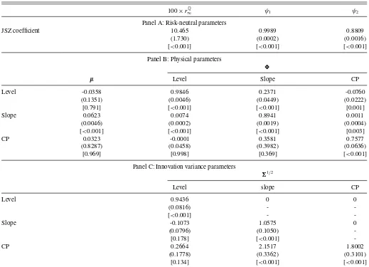
6.2 Parameter Estimates
Table 1reports the parameter estimates of our three-factor GDTSM and, specifically, Panel A presents the estimates of the risk-neutral parameters under the JSZ normalization. The largest eigenvalue of Q is almost equal to one (0.9983), a feature needed to explain the existence of the level factor in interest rates. Specifically, long rates are essentially expected future short-term interest rates under the risk-neutral measure corrected by a Jensen’s inequality term. Hence, the very persis-tent dynamics underQimply that shocks to the first principal component raise expected future rates in parallel, making sense of the level factor of interest rates (see Cochrane and Piazzesi
2008). On the other hand, this extreme persistence makes infer-ence about the risk-neutral long-run mean of the short rate very difficult (see Hamilton and Wu2012), which is reflected in an estimatedrQ
∞that is unusually high.
We also check the model fit across the full spectrum of maturi-ties. Specifically, the root mean squared pricing error (RMSPE) of the model implied by the CGLS estimates is 11.80 basis
Table 1. Parameter estimates
100×rQ
∞ ψ1 ψ2
Panel A: Risk-neutral parameters
JSZ coefficient 10.465 0.9989 0.8809
(1.730) (0.0002) (0.0016)
[<0.001] [<0.001] [<0.001]
Panel B: Physical parameters
µ Level Slope CP
Level -0.0358 0.9846 0.2371 -0.0760
(0.1351) (0.0046) (0.0449) (0.0222)
[0.791] [<0.001] [<0.001] [0.001]
Slope 0.0623 0.0074 0.8941 0.0011
(0.0046) (0.0002) (0.0019) (0.0004)
[<0.001] [<0.001] [<0.001] [0.003]
CP 0.0323 -0.0001 0.3581 0.7577
(0.8287) (0.0458) (0.3982) (0.0636)
[0.969] [0.998] [0.369] [<0.001]
Panel C: Innovation variance parameters
1/2
Level slope CP
Level 0.9436 0 0
(0.0816) -
-[<0.001] -
-Slope -0.1073 1.0575 0
(0.0796) (0.1050)
-[0.178] [<0.001]
-CP 0.2664 2.1517 1.8002
(0.1778) (0.3362) (0.3101)
[0.134] [<0.001] [<0.001]
NOTE: Data are sampled quarterly from 1986Q1 to 2012Q2. Asymptotic standard errors are given in parentheses, and asymptoticp-values in square brackets.
points (bps), which is only marginally worse than the 11.64 bps RMSPE of the reduced-form model. This is confirmed when we look at mean absolute pricing errors (MAPEs). In this case, we have 8.20 versus 7.99 bps. Hence, the loss from imposing the no-arbitrage conditions is minimal: the difference in pricing errors is less than one basis point. In fact, since the risk-neutral measure parameters are pinned down by the cross-section of interest rates, this accuracy in fitting bond yields translates into tight standard errors around these estimates (see Panel A of Ta-ble 1). We also note that the OLS estimates of the model imply RMSPEs and MAPEs of 12.48 and 8.50 bps, respectively. While the model fit is worse than under the CGLS estimation, we note that the loss from using the simpler estimator is minimal. This result is even more compelling once we recall that the OLS estimates do not impose self-consistency.
We now turn our focus to the estimates of the parame-ters driving the physical dynamics of the factors (Panel B of
Table 1). We find that the level factor is very persistent, with a 0.98 coefficient, while the slope coefficient decays somewhat faster, with a 0.90 coefficient. Finally, the return-forecasting factor is the least persistent factor, with a 0.76 coefficient.
The estimated dynamics seem to be consistent with those found by Cochrane and Piazzesi (2008) for the United States. First, a change in the level factor does not seem to have an impact on anything else: the effect of a change in the level factor on the slope is 0.0074, while the effect on the return-forecasting factor is−0.0011. Second, the return-forecasting factor seems to set off a small effect on the level but not on the slope. Finally, a movement in the slope affects all three factors. For example, the coefficient that measures the effect of a change in the slope on the return-forecasting factor is 0.36. This implies that, even if current expected returns are zero today, one would forecast high future returns when the term structure is upward sloping. However, we have to be careful in interpreting this result, since this coefficient is measured with great imprecision.
Also, it is interesting to analyze the effects of the restrictions on the prices of risk and the bias correction of the reduced-form parameters on the estimated persistence of this system. In particular, we find that the estimated persistence of a model with unrestricted VAR(1) dynamics underPis 0.9897. Impos-ing the CP-like restrictions, on the other hand, increases the estimated persistence only marginally (0.9905). Finally, a com-bined approach of the price of risk restrictions and bias correc-tions pushes the persistence up to 0.9938.
We can use the fact that the minimized value of the ALS criterion function has an asymptoticχ2distribution to test the
validity of the model. Specifically, we have that the dimension-ality of the distance function is 198, the number of parameters of interest is 27 and there are six additional restrictions imposed by the CP single-factor structure of excess returns. This leaves 165 degrees of freedom. The 1% (5%) critical value for aχ2(165) is 210.17 (195.97), while the minimized value of the ALS crite-rion is 166.76. Hence, there is no evidence that the restrictions imposed by the model are inconsistent with the data.
We also test the validity of the CP restrictions using an ALS-based distance metric test. In particular, we calculate the dif-ference between the ALS criterion function evaluated at the estimate that imposes the self-consistency and CP restrictions, and the ALS criterion function evaluated at an estimate that only
imposes the self-consistency restrictions. We note that both es-timates have been computed using the same weighting matrix. This difference has an asymptoticχ2 distribution with six
de-grees of freedom (i.e., the number of restrictions). The 1% (5%) critical value for aχ2(6) is 16.81 (12.59), while the difference between the ALS criteria is 1.26. Thus, we do not find evidence against the CP restrictions.
Last and consistent with the results reported in Hamilton and Wu (2014) for the case of the U.S. yield curve, we find evidence of serial correlation in the yield fitting errors. To address this issue, we could estimate the covariance of the reduced-form parameters in (14) using a method that is robust to autocorrela-tion. However, mirroring the case of GMM estimation of highly overidentified models, the optimal weighting matrix is likely to be poorly estimated when the number of reduced-form parame-ters is large, thus leading to poor finite sample properties of the estimator. Specifically, since sampling error in the small eigen-values is magnified in the process of inversion of the weighting matrix, one could follow Doran and Schmidt (2006) and use principal component analysis to remove these terms to decrease the variance of the estimated weighting matrix. We leave such an approach for further research.
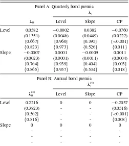
6.3 Prices of Risk
Estimates of the prices of risk subject to the CP restrictions are shown inTable 2. Panel A focuses on the (quarterly) price of risk coefficients. We find that both the level and slope fac-tors are priced, and that their prices of risk are solely driven by
Table 2. Price of risk estimates
Panel A: Quarterly bond premia
λ1
λ0 Level Slope CP
Level 0.0582 −0.0002 0.0382 −0.0760
(0.1351) (0.0046) (0.0449) (0.0222)
[0.667] [0.960] [0.395] [<0.001]
{0.823} {0.973} {0.526} {0.011}
Slope −0.0007 0.0001 −0.0009 0.0011
(0.0023) (0.0001) (0.0011) (0.0004)
[0.764] [0.939] [0.404] [0.003]
{0.865} {0.957} {0.534} {0.018}
Panel B: Annual bond premia
λ(4)1
λ(4)0 Level Slope CP
Level 0.2216 0 0 −0.2037
(0.3823) - - (0.0516)
[0.562] - - [<0.001]
{0.816} - - {0.008}
Slope 0 0 0 0
- - -
-- - -
-- - -
-NOTE: Data are sampled quarterly from 1986Q1 to 2012Q2. Asymptotic standard errors are given in parentheses, asymptoticp-values in square brackets and bootstrapp-values in curly brackets.