Full Terms & Conditions of access and use can be found at
http://www.tandfonline.com/action/journalInformation?journalCode=ubes20
Download by: [Universitas Maritim Raja Ali Haji] Date: 11 January 2016, At: 18:49
Journal of Business & Economic Statistics
ISSN: 0735-0015 (Print) 1537-2707 (Online) Journal homepage: http://www.tandfonline.com/loi/ubes20
Estimating Conditional Average Treatment Effects
Jason Abrevaya, Yu-Chin Hsu & Robert P. Lieli
To cite this article: Jason Abrevaya, Yu-Chin Hsu & Robert P. Lieli (2015) Estimating Conditional Average Treatment Effects, Journal of Business & Economic Statistics, 33:4, 485-505, DOI: 10.1080/07350015.2014.975555
To link to this article: http://dx.doi.org/10.1080/07350015.2014.975555
Accepted author version posted online: 30 Oct 2014.
Published online: 27 Oct 2015. Submit your article to this journal
Article views: 233
View related articles
Estimating Conditional Average
Treatment Effects
Jason A
BREVAYADepartment of Economics, University of Texas, Austin, TX 78712 ([email protected])
Yu-Chin H
SUInstitute of Economics, Academia Sinica, Taipei 115, Taiwan ([email protected])
Robert P. L
IELIDepartment of Economics, Central European University, H-1051 Budapest, Hungary and Magyar Nemzeti Bank, 1850 Budapest, Hungary ([email protected])
We consider a functional parameter called the conditional average treatment effect (CATE), designed to capture the heterogeneity of a treatment effect across subpopulations when the unconfoundedness assumption applies. In contrast to quantile regressions, the subpopulations of interest are defined in terms of the possible values of a set of continuous covariates rather than the quantiles of the potential outcome distributions. We show that the CATE parameter is nonparametrically identified under unconfoundedness and propose inverse probability weighted estimators for it. Under regularity conditions, some of which are standard and some are new in the literature, we show (pointwise) consistency and asymptotic normality of a fully nonparametric and a semiparametric estimator. We apply our methods to estimate the average effect of a first-time mother’s smoking during pregnancy on the baby’s birth weight as a function of the mother’s age. A robust qualitative finding is that the expected effect becomes stronger (more negative) for older mothers.
KEY WORDS: Birth weight; Inverse probability weighted estimation; Nonparametric method; Treatment effect heterogeneity.
1. INTRODUCTION
When individual treatment effects in the population are het-erogeneous, but treatment assignment is unconfounded given a vectorX of observable covariates, it is a well-known result that the average treatment effect (ATE) in the population is non-parametrically identified (see, e.g., Rosenbaum and Rubin1983, 1985). Given the heterogeneity of individual effects, it may also be of interest to estimate ATE in various subpopulations defined by the possible values of some component(s) ofX. We will refer to the value of the ATE parameter within such a subpopulation as a conditional average treatment effect (CATE). For example, if one of the covariates is gender, one might be interested in estimating ATE separately for males and females. As treatment assignment in the two subpopulations is unconfounded given the rest of the components ofX, one can simply split the sam-ple by gender and apply standard nonparametric estimators of ATE to the two subsamples. A second example, considered by a number of authors, is to define CATE as a function of the full set of conditioning variablesX. In this case CATE(x) gives the conditional mean of the treatment effect for any pointxin the support ofX.
Though not referred to by this name, the CATE function in-troduced in the second example already appears in Hahn (1998) and Heckman, Ichimura, and Todd (1997,1998) as a “first stage” estimand in the (imputation-based) nonparametric estimation of ATE. Heckman and Vytlacil (2005) discussed the identification and estimation of CATE(x), which they called ATE(x), in terms of the marginal treatment effect in a general structural model. Khan and Tamer (2010) mentioned CATE(x) explicitly, but their
focus was on ATE. Lee and Whang (2009) and Hsu (2012) considered estimating and testing hypotheses about CATE(x) whenXis absolutely continuous, and provided detailed asymp-totic theory. MaCurdy, Chen, and Hong (2011) also discussed the identification and estimation of CATE(x).
In this article we extend the concept of CATE to the tech-nically more challenging situation in which the conditioning covariatesX1are continuous and form a strict subset ofX. As
the unconfoundedness assumption will not generally hold con-ditional onX1alone, it is not possible to simply apply, say, the
Lee and Whang (2009) CATE estimator withX1 playing the
role ofX. Rather, one needs to estimate CATE as a function of
X, and then average out the unwanted components by integrat-ing with respect to the conditional distribution ofX(1)givenX1,
where X(1) denotes those components ofX that are not inX1.
This distribution is, however, generally unknown and has to be estimated.
WhenX1is a discrete variable (such as in the first example),
averaging with respect to the empirical distribution ofX(1)|X1
is accomplished “automatically” by virtue of the ATE estimator being implemented subsample-by-subsample. The result is an estimate of CATE(x1) for each pointx1 in the support ofX1.
This suggests that when X1 is continuous one could at least
© 2015American Statistical Association Journal of Business & Economic Statistics
October 2015, Vol. 33, No. 4 DOI:10.1080/07350015.2014.975555
Color versions of one or more of the figures in the article can be found online atwww.tandfonline.com/r/jbes.
485
approximate CATE by discretizingX1 and estimating ATE on
the resulting subsamples provided that they are large enough. However, the CATE estimate obtained this way will depend on the discretization used and will be rather crude and discontinu-ous, just as a histogram is generally a crude and discontinuous estimate of the underlying density function.
The technical contribution of this article consists of propos-ing “smooth” nonparametric and semiparametric estimators of CATE whenX1is continuous and a strict subset ofX, and
devel-oping the first-order asymptotic theory of these estimators. The estimators are constructed as follows. First, the propensity score, the probability of treatment conditional onX, is estimated by ei-ther a kernel-based regression (the fully nonparametric case) or by a parametric model (the semiparametric case). In the second step the observed outcomes are weighted based on treatment status and the inverse of the estimated propensity score, and local averages are computed around points in the supportX1,
using another set of kernel weights. (Intuitively, the second stage can be interpreted as integrating with respect to a smoothed es-timate of the conditional distribution of the inverse propensity weighted outcomes givenX1.) Under regularity conditions the
estimator is shown to be consistent and asymptotically normal; the results allow for pointwise inference about CATE as a func-tion of X1. Of the conditions used to prove these results, the
most noteworthy ones are those that are used in the fully non-parametric case to restrict the relative convergence rates of the two smoothing parameters employed in steps one and two, and prescribe the order of the kernels.
The CATE estimators described above can be regarded as gen-eralizations of the inverse probability weighted ATE estimator proposed by Hirano, Imbens, and Ridder (2003). An alternative (first-order equivalent) estimator of CATE could be based on nonparametric imputation (e.g., Hahn1998). In this article we restrict attention to the first approach.
We present simulation results as well as an empirical exercise to illustrate the finite sample properties and the practical imple-mentation of our estimators. Specifically, we estimate the ex-pected effect of a first-time mother’s smoking during pregnancy on the birth weight of her child conditional on the mother’s age, using vital statistics data from North Carolina. In this exercise we focus on the semiparametric estimator, as in most applied settings, such as the one at hand, the applicability of a fully nonparametric procedure is likely to be hampered by curse of dimensionality problems.
The intended contribution of the application to the pertain-ing empirical literature is to explore the heterogeneity of the smoking effect along a given dimension in an unrestricted and intuitive fashion. Previous estimates reported in the literature are typically constrained to be a single number by the func-tional form of the underlying regression model. If the effect of smoking is actually heterogeneous, such an estimate is of course not informative about how much the effect varies across relevant subpopulations and may not even be consistent for the overall population mean.
Nevertheless, there have been some attempts in the literature to capture the heterogeneity of the treatment effect in question. Most notably, Abrevaya and Dahl (2008) estimated the effect of smoking separately for various quantiles of the birth weight dis-tribution. Though insightful, a drawback of the quantile regres-sion approach is that it allows for heterogeneity in the treatment
effect across subpopulations that are not identifiable based on the mother’s characteristics alone. Hence, the estimated effects are hard to translate into targeted “policy” recommendations. For instance, Abrevaya and Dahl (2008) reported that the negative effect of smoking on birth weight is more pronounced at the me-dian of the birth weight distribution than at the 90th percentile. However, it is not clear, before actual birth, or at least without additional modeling, which quantile should be “assigned” to a mother with a given set of observable characteristics. In addi-tion, the treatment effect for any given quantile could also be a function of these characteristics (this is assumed away by the linear specification they use). In contrast, the CATE parameter is defined as a function of variables that are observable a pri-ori, and the estimator proposed in this article places only mild restrictions on the shape of this function.
Qualitatively, the main story that emerges from our empirical exercise is that the predicted average effect of smoking becomes stronger (more negative) at higher age. This finding is reason-ably robust with respect to race, smoothing parameters, and the specification of the propensity score. Nevertheless, there is a fair amount of specification and estimation uncertainty about the numerical extent of this variation.
The rest of the article is organized as follows. Section2 intro-duces the CATE parameter and discusses its identification and estimation. The first-order asymptotic properties of the proposed estimators are developed. Section3presents the simulation re-sults, and Section4is devoted to the empirical exercise. Section 5outlines possible extensions of the basic framework, includ-ing multivalued treatments and instrumental variables. Section 6concludes.
2. THEORY
2.1 The Formal Framework and the Proposed Estimators
LetDbe a dummy variable indicating treatment status in a population of interest withD=1 if an individual (unit) receives treatment andD=0 otherwise. DefineY(1) as the potential outcome for an individual if treatment is imposed exogenously;
Y(0) is the corresponding potential outcome without treatment. LetXbe ak-dimensional vector of covariates withk≥2. The econometrician observesD,X, andY ≡D·Y(1)+(1−D)·
Y(0). In particular, we make the following assumption.
Assumption 1 (Sampling). The data, denoted {(Di, Xi, Yi)}ni=1, is a random sample of size n from the joint
dis-tribution of the vector (D, X, Y).
Throughout the article we maintain the assumption that the observed vectorXcan fully control for any endogeneity in treat-ment choice. Stated formally:
Assumption 2 (Unconfoundedness). (Y(0), Y(1))⊥DX.
Assumption 2 is also known as (strongly) “ignorable treat-ment assigntreat-ment” (Rosenbaum and Rubin 1983), and it is a rather strong but standard identifying assumption in the treat-ment effect literature. In particular, it rules out the existence of unobserved factors that affect treatment choice and are also correlated with the potential outcomes.
Let X1∈Rℓ be a subvector of X∈Rk, 1≤ℓ < k, X
ab-solutely continuous. Theconditional average treatment effect
(CATE) givenX1=x1is defined as
τ(x1)≡E[Y(1)−Y(0)|X1=x1].
Under Assumption 2, τ(x1) can be identified from the joint
distribution of (X, D, Y) as
τ(x1)=E[E[Y|D=1, X]−E[Y|D=0, X]|X1 =x1] (1)
or
τ(x1)=E
DY
p(X)−
(1−D)Y
1−p(X)
X1=x1
, (2)
wherep(x)=P[D=1|X=x] denotes the propensity score function. These identification results follow from a simple string of equalities justified by the law of iterated expectations and un-confoundedness. While Equation (1) identifies CATE somewhat more intuitively, we will base our estimators on Equation (2).
In particular, we propose the following procedure for esti-matingτ(x1). The first step consists of estimating the propensity
score. We consider two options. Option (i) is a nonparametric es-timator given by a kernel-based (Nadaraya-Watson) regression, that is,
ˆ
p(x)=
1
nhk
n
i=1DiK
Xi−x
h
1
nhk
n
i=1K
Xi−x
h
, (3)
where K(·) is a kernel function andhis a smoothing param-eter (bandwidth). Option (ii) is a parametric estimate ofp(x), for example, a logit or probit model estimated by maximum likelihood.
Given an estimator ˆp(x) for the propensity score, in the second stage we estimateτ(x1) by inverse probability weighting and
kernel-based local averaging, that is, we propose
ˆ
τ(x1)= 1
nhℓ
1 n
i=1
DiYi
ˆ
p(Xi) −
(1−Di)Yi
1−pˆ(Xi) K1
X1i−x1
h1
1
nhℓ
1 n
i=1K1
X1i−x1
h1
,
whereK1(u) is a kernel function andh1is a bandwidth (different
fromKandh). As in the second stage ˆp(x) is evaluated at the sample observationsXi, in the nonparametric case we employ the “leave-one-out” version of (3).
As far as econometric theory is concerned, it is the develop-ment of the asymptotics of the fully nonparametric case that is the central contribution of this article. Though the asymptotics are less novel and challenging, the semiparametric estimator is easier to implement and a more robust practical alternative (at the cost of potential misspecification bias and loss of efficiency). Even though we work out the asymptotic theory of ˆτ(x1) for
anyℓ < k, in our assessment the most relevant case in practice isℓ=1 (and maybe ℓ=2). When X1 is a scalar, ˆτ(x1) can
easily be displayed as a two-dimensional graph while for higher dimensionalX1the presentation and interpretation of the CATE
estimator can become rather cumbersome.
2.2 CATE in a Linear Regression Framework
The standard linear regression model for program evaluation combines a weaker version of the unconfoundedness assump-tion with the assumpassump-tion that the condiassump-tional expectaassump-tion of the
potential outcomes is a linear function. As noted by Imbens and Wooldridge (2009), the treatment effect literature has gradually moved away from this baseline model over the last 10–15 years. The main reason is that the estimated average treatment effect can be severely biased if the linear functional form is not correct. Nevertheless, as the general CATE parameter introduced in this article has not yet been in use in the treatment effect literature, it is useful to develop further intuition by relating it to a standard linear regression framework.
Given the vector X of covariates, we can, without loss of generality, write
E[Y(d)|X]=µd+rd(X), d =0,1,
where µd =E[Y(d)] and rd(·) is some function with E[rd(X)]=0. Under the unconfoundedness assumption, the
mean of the observed outcome conditional onDandX can be represented as
E(Y |X, D)=µ0+(µ1−µ0)D+r0(X)
+[r1(X)−r0(X)]D. (4)
If one assumes r0(X)=[X−E(X)]′β and r1(X)=[X− E(X)]′(β+δ), then CATE(X1) is given by
CATE(X1)=µ1−µ0+E[(X−E(X))′|X1]δ.
Further assuming that the above conditional expectation w.r.t.
X1is a linear function ofX1gives rise to a three-step parametric
estimator of CATE. The first step consists of regressingYon a constant,D,XandD·(X−X¯); specifically, we write
Yi =κˆ+αDˆ i+X′iβˆ+Di(Xi−X¯)′δˆ+ǫˆi, i=1, . . . , n.
(5) The second step consists of regressing each component ofX−
¯
Xon a constant andX1:
X(ij)−X¯(j)=X˜1′iγˆ(j)+uˆi(j), i=1, . . . , n, j =1, . . . , k,
(6) where ˜X1≡(1, X′1)′, andX
(j)and ¯X(j) denote thejth
compo-nent ofX and ¯X, respectively. Finally, forX1=x1, one takes
ˆ
α+( ˜x′1γˆ) ˆδ (7)
as an estimate of CATE(x1), where ˆγ ≡( ˆγ(1), . . . ,γˆ(k)) is an
(ℓ+1)×kmatrix.
The special case in whichδ=0, that is,r0(X)=r1(X),
cor-responds to assuming that individual treatment effects do not systematically depend onX. Accordingly, CATE reduces to a constant function whose value is equal to ATE=µ1−µ0
ev-erywhere, and ATE itself can be estimated as the coefficient on
Dfrom regression (5) without the interaction terms.
Though it requires entirely standard methods, calculating the standard error of (7) is somewhat cumbersome. Specifically, one can write the k+1 regressions in (5) and (6) as a SUR system (see, e.g., Wooldridge 2010, Ch. 7) and estimate the joint variance-covariance matrix of all regression coefficients. Then one can invoke the multivariate delta method to obtain the standard error of (7) for any given x1. The construction
is described in detail inAppendix A. Alternatively, one could resample from the empirical distribution of the residuals and compute bootstrapped standard errors.
2.3 Asymptotic Properties of ˆτ(x1): The Fully Nonparametric Case
In the fully nonparametric case we estimate the propensity score by a kernel-based nonparametric regression:
Assumption 3 (Estimated propensity score). ˆp(Xi) is given by the leave-i-out version of the estimator in (3).
We derive the asymptotic properties of the resulting CATE estimator under the following regularity conditions.
Assumption 4 (Distribution ofX). The supportX of thek -dimensional covariateXis a Cartesian product of compact in-tervals, and the density ofX,f(x), is bounded away from 0 on X.
Letsands1denote positive even integers such thats≥kand s1≥k.
Assumption 5 (Conditional moments and smoothness). (i) supx∈X E[Y(j)2|X=x]<∞ for j =0,1; (ii) the functions mj(x)=E[Y(j)|X=x],j =0,1 andf(x) ares-times con-tinuously differentiable onX.
Assumption 6 (Population propensity score). (i) p(x) is bounded away from 0 and 1 on X; (ii) p(x) is s-times con-tinuously differentiable onX.
A functionκ :Rk
→Ris a kernel of ordersif it integrates to one overRk, andup1
1 ·. . .·u
pk
k κ(u)du=0 for all nonnegative
integersp1, . . . , pksuch that 1≤
ipi < s.
Assumption 7 (Kernels).
(i) K(u) is a kernel of orders, is symmetric around zero, is equal to zero outside ki=1[−1,1], and is continuously
differentiable.
(ii) K1(u) is a kernel of orders1, is symmetric around zero,
and isstimes continuously differentiable.
Assumption 8 (Bandwidths). The bandwidthshandh1satisfy
the following conditions asn→ ∞:
(i) h→0 and log(n)/(nhk+s)
→0. (ii) nh2s1+ℓ
1 →0 andnhℓ1→ ∞.
(iii) h2sh−2s−ℓ
1 →0 andnh ℓ
1h2s →0.
Define the functionψ(x, y, d) as
ψ(x, y, d)≡ d(y−m1(x))
p(x) −
(1−d)(y−m0(x))
1−p(x) +m1(x)−m0(x).
The following theorem states our main theoretical result. The proof is given inAppendices BandC.
Theorem 1. Suppose that Assumptions 1 through 8 are satis-fied. Then, for each pointx1in the support ofX1,
(a)
nhℓ1( ˆτ(x1)−τ(x1)) =
1
nhℓ1
1
f1(x1) n
i=1
[ψ(Xi, Yi, Di)
−τ(x1)]K1
X1i−x1 h1
+op(1)
(b)
nhℓ1( ˆτ(x1)−τ(x1)) d
→N
0,K1 2 2σ
2
ψ(x1)
f1(x1)
,
wheref1(x1) is the pdf ofX1,K12≡(
K1(u)2du)1/2, and
σψ2(x1)≡E[(ψ(X, Y, D)−τ(x1))2|X1=x1].
Comments
1. The technical restrictions imposed on the distribution ofX
and on various conditional moment functions in Assumptions 4 and 5 are analogous to those in Hirano, Imbens, and Ridder (2003) and are common in the literature on nonparametric estimation. As pointed out by Khan and Tamer (2010), the assumption that the propensity score is bounded away from zero and one plays an important role in determining the convergence rate of inverse probability weighted estimators. 2. Assumptions 7(i) and 8(i) ensure that pˆ(x)−p(x)=
op(hs/2), uniformly in x; see Lemma 6.1 part (b) in
Ap-pendix B. This is the convergence rate needed to establish the influence function representation in Theorem 1(a). The influence function itself is analogous to the influence function that efficient nonparametric estimators of ATE possess; see, for example, Hahn (1998) and Hirano, Imbens, and Ridder (2003).
3. The influence function [ψ(Xi, Yi, Di)−τ(x1)]K1
X1i−x1
h1
does not have mean zero; rather, it decomposes into a “bias term” that depends on h1 and a mean zero term to which
Lyapunov’s CLT directly applies. Assumptions 7(ii) and 8(ii) ensure the asymptotic negligibility of the bias term (and the applicability of the CLT). SeeAppendix Cfor further details. 4. Assumption 8(iii) underlies the novel aspects of our asymp-totic theory. It controls the relative and “joint” convergence rates of h (the bandwidth used to estimate the propensity score) andh1 (the bandwidth used in the integration step).
These rates, along with the kernel orders, are chosen subject to numerous tradeoffs that need to be considered to ensure the asymptotic negligibility of all remainder terms in our expansion of ˆτ(x1).
5. More specifically, our asymptotic analysis builds on the ex-pansion of the Hirano, Imbens, and Ridder (2003) ATE es-timator by Ichimura and Linton (2005). However, the in-tegration step causes the factor K1(·/ h1) to appear in each
term, which has a number of consequences. First, the leading
terms in the expansion converge at the rate of
nhℓ
1rather
than √n. Second, as the convergence rates of the original remainder terms depend on h, the presence of K1 and the
scaling by
nhℓ
1 introduce interactions betweenhandh1.
These interactions require thath1converges to zero slower
thanh. In particular, if one were to seth1equal to a constant,
then all remainder terms could be made to vanish by requir-ingh→0 at an appropriate rate as in Ichimura and Linton (2005) or Donald, Hsu, and Lieli (2014b). However, the bias in the leading term, described in comment 3 above, would of course not disappear. Hence, one also needsh1→0, but
slowly enough to satisfy part two of Assumption 8(ii) and part one of 8(iii). One can then employ a kernelK1of
suf-ficiently high order to satisfy the first part of Assumption 8(ii), and a kernelKof sufficiently high order to satisfy part two of Assumption 8(iii), which is needed to ensure that the (conditional) bias of ˆp(x) remains asymptotically negligible
when scaled by
nhℓ
1. Note, however, that increasings, the
order ofK, is not costless—it slows the convergence ofhto zero via Assumption 8(i), which then slows the convergence ofh1to zero via the first part of 8(iii), which again requires
an increase ins1and possiblys, etc.
6. We have yet to show that there actually exist bandwidth sequences and kernel orders satisfying all the requirements posed by Assumption 8 (otherwise the asymptotic theory would be vacuous). We set
h=a·nk+−s1+δ, a >0, δ >0,
h1=a1·n −1
ℓ+2s1−δ1, a1>0, δ1>0,
whereδandδ1can be made as small as necessary or desired. It
is clear that Assumptions 8(i) and (ii) hold with these choices. To satisfy Assumption 8(iii), we further set the kernel orders ass=kforkeven,s=k+1 forkodd, ands1=s+2.
To verifyh2sh−2s−ℓ
1 →0, note thatδ andδ1 can be
arbi-trarily small, so it is sufficient to check
−2s sufficient to check the latter. Again, since δ andδ1 can be
arbitrarily small, we only need
−s
7. To use Theorem 1 for statistical inference, one needs to con-sistently estimateσ2
ψ(x1) andf1(x1). The latter is easily
ac-a uniformly consistent estimac-ator for m1(x) overX in that
supx∈X|mˆ1(x)−m1(x)| =op(1). Similarly, let ˆm0(x) and
ˆ
p(x) be uniformly consistent estimators form0(x) andp(x)
overX. In particular, the ˆp(x) we use is uniformly consis-tent forp(x). Also, such ˆm1(x) and ˆm0(x) can be obtained
by performing kernel regressions ofYonXin the treated and
nontreated subpopulations, respectively. Then, we estimate
σ2
will disappear in the limit.
8. Assumption 4 does not allowXto have discrete components, which is of course restrictive in applications. One way to incorporate discrete covariates into the analysis is as fol-lows. For concreteness, suppose that in addition to some continuous variables,X contains gender. Let M denote the indicator of the male subpopulation and define p(x, m)=
P(D=1|X=x, M =m) form=0,1. We can estimate these functions by kernel based regressions ofDonXin each subsample:
In particular, as we show inAppendix D, the following in-fluence function representation applies to ˆτ(x1):
where
ψ(Mi, Xi, Yi, Di)≡ Di(Yi−m(Xi, Mi))
p(Xi, Mi)
−(1−Di)(Yi−m0(Xi, Mi)) 1−p(Xi, Mi) +m1(Xi, Mi)−m0(Xi, Mi),
andmj(x, m)≡E[Y(j)|X=x, M=m] for j =0,1 and m=0,1. Therefore, Theorem 1 continues to hold for (9) after replacingψ(Xi, Yi, Di) withψ(Mi, Xi, Yi, Di).
9. Kernels satisfying Assumption 7 can be constructed by tak-ing products of higher order univariate kernels. A general method for obtaining higher order kernels from “regular” ones is described, for example, by Imbens and Ridder (2009). The “support” condition imposed onK is for expositional convenience only; we can extend the proof of Theorem 1 to kernels with exponential tails.
2.4 Asymptotic Properties of ˆτ(x1): The Semiparametric Case
The asymptotic theory of estimating CATE simplifies con-siderably if a parametric model is postulated for the propensity score. In particular, we replace Assumption 3 with the following.
Assumption 9 (Parametric propensity score estimator). The estimator ˆθn of the propensity score model p(x;θ),θ∈⊂
Rd,d <
∞, satisfies supx∈X|p(x; ˆθn)−p(x;θ0)| =Op(n−1/2)
whereθ0∈such thatp(x)=p(x;θ0) for allx ∈X.
Assumption 9 will typically hold for standard parametric es-timation methods under reasonably mild regularity conditions. For example, a logit model or a probit model based on a linear index and estimated by maximum likelihood will satisfy (9) if Xis bounded. Obviously, Assumption 9 eliminates the need for those conditions stated in Section2.3whose role is to govern the behavior of the Nadaraya–Watson regression estimator and the interaction between the two bandwidths. Of course, the band-widthh1used in the second, local averaging, stage still needs to
be controlled to ensure consistency and asymptotic normality. Assumption 8(ii) with anys1≥2 is sufficient in this regard.
To state the result formally, define
ψθ(x, y, d)≡ dy p(x)−
(1−d)y
1−p(x).
The following theorem corresponds closely to Theorem 1.
Theorem 2. Suppose that Assumptions 1, 2, 8(ii), and 9 are satisfied for somes1≥2. Then, under some additional regularity
conditions, the following statements hold for each pointx1 in
the support ofX1:
(a)
nhℓ1( ˆτ(x1)−τ(x1)) =
1
nhℓ
1
1
f1(x1) n
i=1
[ψθ(Xi, Yi, Di)
−τ(x1)]K1
X
1i−x1 h1
+op(1)
(b)
nhℓ1( ˆτ(x1)−τ(x1)) d
→N
0,K1 2 2σ
2
ψθ(x1)
f1(x1)
,
wheref1(x1) is the pdf ofX1,K12≡(
K1(u)2du)1/2, and
σψ2
θ(x1)≡E[(ψθ(X, Y, D)−τ(x1))
2
|X1=x1].
The proof of Theorem 2 is given inAppendix E.
Comments
1. The form of the influence function highlights an important difference between estimating ATE and CATE. If ATE is estimated by inverse probability weighting, then even a√n -consistent parametric estimate of the propensity score will make a nontrivial contribution to the influence function (since the ATE estimator itself converges at the same rate). In con-trast, the CATE estimator converges at a rate slower than √n
, so employing a (correctly specified) parametric estima-tor is asymptotically equivalent to the propensity score being known.
2. The semiparametric approach offers several practical advan-tages over the fully nonparametric estimator: (i) It can help circumvent the curse of dimensionality problem whenXis large. (ii) Discrete and continuous covariates can be treated the same way, that is, one can simply include, say, a gender dummy in a logit or probit regression rather than follow the partitioning approach described in comment 8 after Theo-rem 1. This is very useful if one of the categories has a small number of observations. (iii) Only the bandwidth used in the integration step needs to be chosen.
3. Of course, the advantages listed above do not come without costs. While the semparametric approach is still reasonably flexible, misspecification of the score function will generally bias the resulting CATE estimates. Furthermore, the semi-parametric CATE estimator is less efficient than the nonpara-metric one. In particular, we can show that
σψ2(x1)=E
(m1(X)−m0(X)−τ(x1))2+ σ12(X)
p(X)
+ σ
2 0(X)
1−p(X)
X1=x1
,
σψ2
θ(x1)=σ
2
ψ(x1)+E
p(X)(1−p(X))
m1(X)
p(X)
+ m0(X) 1−p(X)
2
X1 =x1
,
where σ2
d(x)=var(Y(d)|X=x) for d =0 and 1. Hence,
clearly σ2
ψθ(x1)≥σ
2
ψ(x1). Therefore, for a given choice of h1 andK1 satisfying the conditions in Theorems 1 and 2,
the semiparametric CATE estimator is less efficient. This result is not surprising given that the influence function of the semiparametric estimator is the same as if p(x) were known (see comment 1 above). It is well known from the work of Hahn (1998) and Hirano, Imbens, and Ridder (2003) that such estimators of ATE do not attain the semiparametric efficiency bound constructed with or without the knowledge ofp(x).
4. The “additional regularity conditions” mentioned in the the-orem are needed to ensure that (i) Lyapunov’s CLT can be applied to the leading term (A.17) in the expansion of the estimator inAppendix E, and (ii) that the remainder term is
−0.5 −0.4 −0.3 −0.2 −0.1 0 0.1 0.2 0.3 0.4 0.5 −0.2
−0.1 0 0.1 0.2 0.3 0.4 0.5
CATE
The true CATE function
0.2 0.3 0.4 0.5 0.6 0.7 0.8 0.9 1 0
200 400 600 800 1000 1200 1400 1600 1800
2000 The distribution of p(X) for k=2
0.5 0.55 0.6 0.65 0.7 0.75 0.8 0.85 0.9 0.95 1 0
0.5 1 1.5
2 2.5x10
6 The distribution of p(X) for k=4
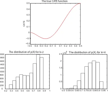
Figure 1. The CATE(x1) function and the distribution ofp(X).
well behaved in that the second factor in (A.18) is Op(1). A set of primitive sufficient conditions could be obtained by suitable changes to Assumptions 4, 5, 6, and 7(ii).
5. K1no longer needs to be a higher order kernel in the
semi-parametric case, but such kernels could still be used in practice.
3. MONTE CARLO SIMULATIONS
In this section we present a Monte Carlo exercise aimed at evaluating the finite sample accuracy of the asymptotic approx-imations given in Theorems 1 and 2. Part of the design is ad-mittedly artificial in that we setk=dim(X)∈ {2,4}, while in practice justifying the unconfoundedness assumption typically requires conditioning on a much larger set of covariates. Never-theless, the setup is rich enough to allow us to make a number of salient and practically relevant points without taking on an undue computational burden. We pay particular attention to ex-ploring the sensitivity of the finite sample distribution of ˆτ(x1)
to the smoothing parameter(s) as first-order asymptotic theory has virtually no implications about how to choose these pa-rameters in practice. Curse of dimensionality issues in the fully nonparametric case are already apparent with four covariates.
3.1 The Data-Generating Process and the Exercise
We consider two data-generating processes (DGPs); one with
k=2 and another withk=4. In the bivariate case the covariates
X=(X1, X2) are given by
X1=ǫ1, X2=(1+2X1)2(−1+X1)2+ǫ2,
where ǫi ∼iid unif[−0.5,0.5], i =1,2. The potential outcomes are defined as
Y(1)=X1X2+ν and Y(0)=0,
where ν∼N(0,0.252) and is independent of (ǫ1, ǫ2). These
definitions imply
CATE(x1)=x1(1+2x1)2(−1+x1)2,
plotted in the top panel ofFigure 1. The propensity score is set asp(X)=(X1+X2), where(·) is the c.d.f. of the logistic
distribution. The distribution of the random variablep(X1, X2)
is shown in the lower left panel ofFigure 1.
To investigate the impact of the curse of dimensionality on our estimator, we also consider the following modification to the DGP:
X1=ǫ1, X2=1+2X1+ǫ2, X3=1+2X1+ǫ3,
X4=(−1+X1)2+ǫ4
Y(1)=X1X2X3X4+ν, Y(0)=0
p(X)=(.5(X1+X2+X3+X4)),
where again ǫi ∼iid unif[−0.5,0.5], i=1,2,3,4 and ν∼ N(0,0.252), independent of theǫ’s. The distribution of the the random variable p(X1, . . . , X4) is shown in lower right panel
ofFigure 1. These modifications leave the CATE(x1) function
unchanged, but make it harder to estimate.
We estimate CATE(x1), x1∈ {−0.4,−0.2,0,0.2,0.4}, for
samples of sizen=500 andn=5000. The number of Monte Carlo repetitions is 1000 in the fully nonparametric case and 5000 in the semiparametric case.
Let T(x1)=√nh1[CATE( x1)−CATE(x1)] and S(x1)=
(T(x1)−ET(x1))/s.e.(T(x1)). For each x1, we report (the
Monte Carlo estimate of) the mean of T(x1)/√nh1 (i.e.,
the raw bias of CATE(x1)), the standard deviation of T(x1),
the estimated standard deviation of T(x1), the MSE of T(x1), the probability that S(x1) exceeds 1.645 and 1.96,
respectively, and the probability that S(x1) is below −1.645
and−1.96, respectively.
We implement the fully nonparametric and semiparametric version of the estimator for various choices of the bandwidthsh
andh1. Motivated by Comment 6 after Theorem 1, fork=2 we
sets=2,s1 =4,h=an−1/4fora ∈ {0.5,0.167,1.5}andh1= a1n−1/9fora1∈ {0.2,0.067,0.6}. Fork=4, the corresponding
choices ares=4,s1=6,h=an−1/8fora∈ {0.5,0.167,1.5}
andh1 =a1n−1/13fora1∈ {0.2,0.067,0.6}. We will refer to the
choicesa =0.5 anda1=0.2 as “baseline;” these values were
calibrated to ensure that forn=5000 the actual distribution of ˆ
τ(x1) is reasonably close to its theoretical limit for most of the
five points considered, as measured by the statistics listed above. We then varyhand/orh1(by tripling and/or thirdingaanda1) to
illustrate how oversmoothing or undersmoothing relative to this crude baseline affects the quality of the inferences drawn from the asymptotic results given in Theorems 1 and 2. Note that in specifying h and h1 as above, we ignore the (small) positive
constantsδandδ1and simply set them to zero.
Regarding further computational details, we use a normal kernel (and higher order kernels derived from it) throughout. In computing the variance of ˆτ(x1), we use the bandwidthhand
a regular kernel to estimate the functions m0 and m1 (in the
fully nonparametric case); the bandwidthh1and the kernelK1
to estimate f1(x1), and the bandwidthh1and a regular kernel
to estimateσ2
ψ(x1) andσψ2θ(x1). The estimated propensity score
is trimmed to lie in the interval [0.005,0.995]. This constraint affects the fully nonparametric estimator forn=500, but it is basically inconsequential for the semiparametric estimator or in larger samples.
There are other relevant issues we do not investigate here in detail due to constraints on space and scope. One is the sensi-tivity of our asymptotic approximations to the propensity score approaching zero or one with high probability. Based on re-sults, both theoretical (Khan and Tamer2010) and experimental (Huber et al. 2012; Donald, Hsu, and Lieli2014a), we expect the asymptotic distributions given in Theorems 1 and 2 to be worse small sample approximations in this case. Another issue not addressed by the simulations is the sensitivity of the semi-parametric estimator to the misspecification of the propensity score model. Nevertheless, the empirical exercise presented in Section4will provide an illustration of the possible impact and handling of these problems in practice.
3.2 Simulation Results
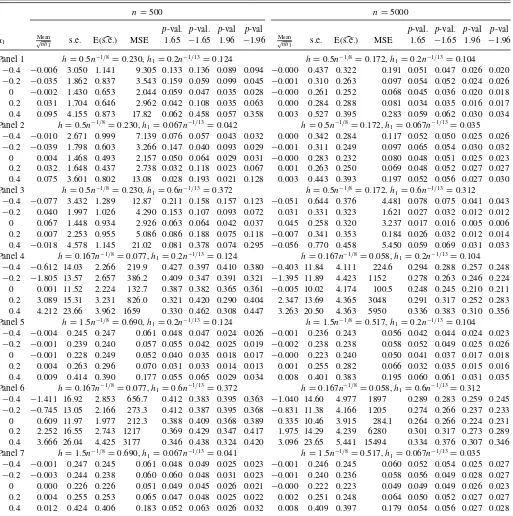
We highlight several aspects of the simulation results reported inTables 1through3.
First, as seen in Panel 1 ofTables 1and2, the distribution of the fully nonparametric estimator for n=5000 is reason-ably close to its theoretical limit under the baseline bandwidth choices, and the studentized estimator leads to reliable infer-ences without major size distortions. In fact, for k=2 the asymptotic theory seems to work well even for n=500, but fork=4 there is a significant improvement in the approxima-tions as one goes fromn=500 ton=5000. In particular, there is a marked reduction in the bias of the estimator at most points
x1, as well as the bias of the estimated standard error. More
generally, comparingTables 1and2across panels provides ev-idence on the curse of dimensionality—for a given sample size, CATE(x1) can be estimated much less precisely in terms of MSE
when the dimensionality ofXis larger, and the asymptotic ap-proximation captures finite sample properties to a much lesser degree. (As explained in the previous section, the bandwidths across the two tables are adjusted for the change in the dimen-sionality ofXby adjusting the exponent ofnbut not the scaling factor.) Viewed somewhat differently, fork=2, results tend to change much less across the two sample sizes, while fork=4, asymptotic theory generally starts “kicking in” much slower.
Second, as can be expected, the bias of ˆτ(x1) is generally
larger ifx1is close to the boundary of the support ofX1.
(More-over, boundary bias is often accompanied by evidence of skew-ness.) Bias can be a result of oversmoothing with a largeh1
(compare, e.g., Panels 1 and 3 in Tables 1 and 2) or under-smoothing with a smallh (compare Panels 1 and 4 inTable 1 and especiallyTable 2). Choosingh too small for the sample size has the additional effect of causing severe bias in the es-timated standard errors, which, in turn, can throw thep-values ofS(x1) completely off. Oversmoothing withh1also biases the
standard errors, but this problem seems much milder in compar-ison. Nevertheless, biased standard errors do not always lead to bad inference. For example, as seen in Panel 1 ofTable 2, for
n=5000 the estimated standard errors are still biased down-ward at points close to the boundary (x1= −0.4 andx1=0.4),
but thep-values of the studentized estimator are very close to their nominal levels. This suggests that the observed s.e. of
T(±0.4) is blown up by just a few outlier estimates.
Third, while Assumption 8(iii) implies that the ratioh/ h1
should go to zero asn→ ∞, the results described in the pre-vious paragraph caution against necessarily imposingh << h1
in practice. Panel 6 in Tables 1 and 2 contains results for h
small andh1large. As expected, there is severe bias in both the
estimator and the standard errors, and inference is misleading (especially fork=4). In contrast, if one takes the opposite ex-treme, that is, oversmooths withhand undersmooths withh1,
as shown in Panel 7 ofTables 1and2, the asymptotic theory delivers very nice approximations even forn=500 andk=4 and despite the fact thath/ h1is very large. This does not mean
that the asymptotics are invalid; it just means, as usual, that first-order asymptotic theory has little to say about how to pick the smoothing parameters in finite samples.
The observation that oversmoothing the propensity score es-timate can be beneficial in finite samples leads naturally to considering the semiparametric version of the estimator. The results are displayed inTable 3.
Our fourth observation then is that the asymptotic normal approximation for the semiparametric estimator performs well
Table 1. The distribution of√nh1[ ˆτ(x1)−τ(x1)]: the fully nonparametric case withk=2
n=500 n=5000
p-val. p-val. p-val p-val p-val. p-val. p-val p-val
x1 √Meannh
1 s.e. E(s.e.) MSE 1.65 −1.65 1.96 −1.96
Mean
√nh
1 s.e. E(s.e.) MSE 1.65 −1.65 1.96 −1.96
Panel 1 h=0.5n−1/4
=0.106,h1=0.2n−1/9=0.100 h=0.5n−1/4=0.059,h1=0.2n−1/9=0.078
−0.4 −0.002 0.337 0.276 0.114 0.074 0.080 0.044 0.047 −0.000 0.277 0.275 0.077 0.051 0.053 0.026 0.028 0.2 0.002 0.245 0.237 0.061 0.059 0.056 0.030 0.026 0.001 0.235 0.235 0.056 0.052 0.050 0.025 0.025 0 0.001 0.213 0.218 0.046 0.050 0.044 0.025 0.022 0.000 0.205 0.211 0.042 0.047 0.044 0.023 0.022 0.2 0.003 0.209 0.215 0.044 0.043 0.044 0.024 0.019 0.000 0.202 0.209 0.041 0.042 0.043 0.021 0.024 0.4 0.001 0.222 0.218 0.049 0.052 0.055 0.027 0.029 0.000 0.210 0.209 0.044 0.048 0.052 0.025 0.027 Panel 2 h=0.5n−1/4
=0.106,h1=0.067n−1/9=0.034 h=0.5n−1/4=0.059,h1=0.067n−1/9=0.026
−0.4 0.002 0.324 0.275 0.105 0.074 0.078 0.043 0.045 0.000 0.287 0.280 0.082 0.052 0.059 0.027 0.029
−0.2 −0.001 0.246 0.233 0.060 0.063 0.060 0.035 0.030 −0.000 0.240 0.233 0.057 0.058 0.055 0.030 0.028 0 −0.000 0.213 0.206 0.045 0.056 0.054 0.030 0.025 −0.000 0.204 0.204 0.042 0.051 0.047 0.025 0.026 0.2 0.001 0.213 0.199 0.045 0.063 0.059 0.035 0.031 0.000 0.208 0.198 0.043 0.058 0.062 0.031 0.033 0.4 0.007 0.238 0.208 0.057 0.071 0.081 0.041 0.042 0.001 0.235 0.207 0.056 0.074 0.072 0.043 0.040 Panel 3 h=0.5n−1/4
=0.106,h1=0.6n−1/9=0.301 h=0.5n−1/4=0.059,h1=0.6n−1/9=0.233
−0.4 −0.042 0.375 0.308 0.405 0.076 0.075 0.046 0.045 −0.038 0.325 0.299 1.746 0.067 0.066 0.037 0.036
−0.2 0.062 0.257 0.259 0.648 0.048 0.047 0.027 0.022 0.033 0.235 0.248 1.344 0.042 0.038 0.021 0.019 0 0.064 0.218 0.248 0.660 0.034 0.031 0.015 0.012 0.038 0.209 0.242 1.743 0.025 0.033 0.009 0.013 0.2 −0.030 0.232 0.258 0.185 0.033 0.033 0.016 0.016 −0.007 0.217 0.245 0.099 0.027 0.030 0.012 0.012 0.4 −0.100 0.272 0.305 1.582 0.030 0.034 0.012 0.017 −0.059 0.258 0.280 4.096 0.036 0.037 0.014 0.017 Panel 4 h=0.167n−1/4
=0.035,h1=0.2n−1/9=0.100 h=0.167n−1/4=0.020,h1=0.2n−1/9=0.078
−0.4 0.074 2.236 0.315 5.271 0.239 0.504 0.225 0.466 0.002 0.334 0.275 0.113 0.080 0.081 0.050 0.051
−0.2 −0.018 0.790 0.237 0.640 0.199 0.179 0.160 0.142 −0.002 0.251 0.235 0.065 0.063 0.059 0.034 0.034 0 −0.000 0.330 0.216 0.109 0.090 0.090 0.060 0.056 0.000 0.210 0.211 0.044 0.052 0.047 0.025 0.025 0.2 0.013 0.247 0.215 0.070 0.059 0.061 0.035 0.033 0.003 0.203 0.209 0.044 0.046 0.041 0.021 0.024 0.4 0.031 0.621 0.224 0.435 0.084 0.142 0.064 0.090 0.003 0.211 0.208 0.049 0.047 0.053 0.026 0.026 Panel 5 h=1.5n−1/4
=0.317,h1=0.2n−1/9=0.100 h=1.5n−1/4=0.178,h1=0.2n−1/9=0.078
−0.4 −0.006 0.273 0.259 0.076 0.059 0.063 0.031 0.035 −0.001 0.268 0.266 0.072 0.051 0.056 0.026 0.029
−0.2 0.006 0.235 0.234 0.057 0.054 0.047 0.027 0.024 0.002 0.237 0.236 0.057 0.054 0.047 0.025 0.026 0 0.001 0.211 0.221 0.044 0.046 0.038 0.023 0.018 0.000 0.204 0.213 0.042 0.044 0.043 0.022 0.020 0.2 0.008 0.218 0.221 0.051 0.047 0.047 0.026 0.021 0.002 0.210 0.210 0.045 0.046 0.052 0.023 0.025 0.4 0.014 0.248 0.230 0.071 0.060 0.064 0.031 0.038 0.007 0.228 0.213 0.069 0.058 0.063 0.034 0.033 Panel 6 h=0.167n−1/4
=0.035,h1=0.6n−1/9=0.301 h=0.167n−1/4=0.020,h1=0.6n−1/9=0.233
−0.4 −0.003 2.354 0.323 5.543 0.259 0.480 0.241 0.442 −0.037 0.421 0.299 1.771 0.103 0.104 0.070 0.065
−0.2 0.073 1.096 0.256 2.011 0.239 0.322 0.220 0.276 0.032 0.259 0.247 1.263 0.059 0.055 0.033 0.027 0 0.066 0.450 0.244 0.856 0.124 0.116 0.093 0.085 0.038 0.215 0.241 1.725 0.029 0.036 0.011 0.015 0.2 −0.020 0.396 0.257 0.216 0.087 0.087 0.059 0.055 −0.005 0.220 0.245 0.074 0.030 0.031 0.013 0.014 0.4 −0.076 0.819 0.311 1.542 0.069 0.118 0.054 0.068 −0.056 0.265 0.280 3.676 0.037 0.041 0.017 0.017 Panel 7 h=1.5n−1/4=0.317,h
1=.067n−1/9=0.034 h=1.5n−1/4=0.178,h1=.067n−1/9=0.026
−0.4 −0.001 0.271 0.255 0.073 0.057 0.064 0.029 0.034 −0.000 0.276 0.270 0.076 0.052 0.057 0.027 0.030
−0.2 0.003 0.236 0.233 0.056 0.058 0.048 0.030 0.024 0.001 0.241 0.235 0.058 0.058 0.054 0.028 0.028 0 −0.000 0.210 0.210 0.044 0.052 0.043 0.029 0.021 −0.000 0.203 0.206 0.041 0.049 0.046 0.023 0.023 0.2 0.006 0.220 0.204 0.049 0.065 0.061 0.035 0.034 0.001 0.214 0.199 0.046 0.063 0.070 0.034 0.035 0.4 0.021 0.252 0.222 0.071 0.066 0.084 0.037 0.045 0.008 0.251 0.212 0.071 0.081 0.082 0.049 0.049
with a fairly wide range of bandwidths, but small choices of
h1 seem to work particular well. Results for the baseline h1
are shown inTable 3, Panel 1 (k=2) and Panel 4 (k=4). In both cases, bias is minimal (even forn=500) and thep-values are acceptable (though there are some instances where they are somewhat below their nominal levels). When one triples h1
relative to baseline (Panels 3 and 6), bias starts creeping into both the estimator and the standard errors, and the p-values become somewhat attenuated. In contrast, as shown by Panels 2 and 5, cuttingh1by a factor of three yields a textbook-perfect
approximation forn=5000. In fact, additional experimentation shows that makingh1an order of magnitude smaller still works
very well.
Fifth, as stated in Comment 3 after Theorem 2, theory predicts that for a given choice ofh1andK1, the asymptotic variance of
the fully nonparametric CATE estimator is smaller than that of the semiparametric one. Comparing the results inTables 1versus 3andTables 2versus3shows that in finite samples the efficiency ranking can go either way, depending also on the choice ofh. Take, for example,k=2 andn=5000 with the baseline choice ofh1(i.e.,h1=0.078). Though the differences are rather small,
in this case the standard error of the nonparametric estimator is indeed smaller than that of the semiparametric estimator almost uniformly inhandx1(compare Panel 1 ofTable 3with Panels
1, 4 and 5 ofTable 1). Exceptions arise only when the nonpara-metric estimator undersmooths the propensity score (Panel 4 of
Table 2. The distribution of√nh1[ ˆτ(x1)−τ(x1)]: the fully nonparametric case withk=4
n=500 n=5000
p-val. p-val. p-val p-val p-val. p-val. p-val p-val
x1 Mean√nh
1 s.e. E(s.e.) MSE 1.65 −1.65 1.96 −1.96
Mean
√nh
1 s.e. E(s.e.) MSE 1.65 −1.65 1.96 −1.96
Panel 1 h=0.5n−1/8
=0.230,h1=0.2n−1/13=0.124 h=0.5n−1/8=0.172,h1=0.2n−1/13=0.104
−0.4 −0.006 3.050 1.141 9.305 0.133 0.136 0.089 0.094 −0.000 0.437 0.322 0.191 0.051 0.047 0.026 0.020
−0.2 −0.035 1.862 0.837 3.543 0.159 0.059 0.099 0.045 −0.001 0.310 0.263 0.097 0.054 0.052 0.024 0.026 0 −0.002 1.430 0.653 2.044 0.059 0.047 0.035 0.028 −0.000 0.261 0.252 0.068 0.045 0.036 0.020 0.018 0.2 0.031 1.704 0.646 2.962 0.042 0.108 0.035 0.063 0.000 0.284 0.288 0.081 0.034 0.035 0.016 0.017 0.4 0.095 4.155 0.873 17.82 0.062 0.458 0.057 0.358 0.003 0.527 0.395 0.283 0.059 0.062 0.030 0.034 Panel 2 h=0.5n−1/8
=0.230,h1=0.067n−1/13=0.042 h=0.5n−1/8=0.172,h1=0.067n−1/13=0.035
−0.4 −0.010 2.671 0.999 7.139 0.076 0.057 0.043 0.032 0.000 0.342 0.284 0.117 0.052 0.050 0.025 0.026
−0.2 −0.039 1.798 0.603 3.266 0.147 0.040 0.093 0.029 −0.001 0.311 0.249 0.097 0.065 0.054 0.030 0.032 0 0.004 1.468 0.493 2.157 0.050 0.064 0.029 0.031 −0.000 0.283 0.232 0.080 0.048 0.051 0.025 0.023 0.2 0.032 1.648 0.437 2.738 0.032 0.118 0.023 0.067 0.001 0.263 0.250 0.069 0.048 0.052 0.027 0.027 0.4 0.075 3.601 0.802 13.08 0.028 0.193 0.021 0.128 0.003 0.443 0.393 0.197 0.052 0.056 0.027 0.030 Panel 3 h=0.5n−1/8
=0.230,h1=0.6n−1/13=0.372 h=0.5n−1/8=0.172,h1=0.6n−1/13=0.312
−0.4 −0.077 3.432 1.289 12.87 0.211 0.158 0.157 0.123 −0.051 0.644 0.376 4.481 0.078 0.075 0.041 0.043
−0.2 0.040 1.997 1.026 4.290 0.153 0.107 0.093 0.072 0.031 0.331 0.323 1.621 0.027 0.032 0.012 0.012 0 0.067 1.448 0.934 2.926 0.063 0.064 0.042 0.037 0.045 0.258 0.320 3.237 0.017 0.016 0.005 0.006 0.2 0.007 2.253 0.955 5.086 0.086 0.188 0.075 0.118 −0.007 0.341 0.353 0.184 0.026 0.032 0.012 0.014 0.4 −0.018 4.578 1.145 21.02 0.081 0.378 0.074 0.295 −0.056 0.770 0.458 5.450 0.059 0.069 0.031 0.033 Panel 4 h=0.167n−1/8
=0.077,h1=0.2n−1/13=0.124 h=0.167n−1/8=0.058,h1=0.2n−1/13=0.104
−0.4 −0.612 14.03 2.266 219.9 0.427 0.397 0.410 0.380 −0.403 11.84 4.111 224.6 0.294 0.288 0.257 0.248
−0.2 −1.805 13.57 2.657 386.2 0.409 0.347 0.391 0.321 −1.395 11.89 4.423 1152 0.278 0.263 0.246 0.224 0 0.001 11.52 2.224 132.7 0.387 0.382 0.365 0.361 −0.005 10.02 4.174 100.5 0.248 0.245 0.210 0.211 0.2 3.089 15.31 3.231 826.0 0.321 0.420 0.290 0.404 2.347 13.69 4.365 3048 0.291 0.317 0.252 0.283 0.4 4.212 23.66 3.962 1659 0.330 0.462 0.308 0.447 3.263 20.50 4.363 5950 0.336 0.383 0.310 0.356 Panel 5 h=1.5n−1/8
=0.690,h1=0.2n−1/13=0.124 h=1.5n−1/8=0.517,h1=0.2n−1/13=0.104
−0.4 −0.004 0.245 0.247 0.061 0.048 0.047 0.024 0.026 −0.001 0.236 0.243 0.056 0.042 0.044 0.024 0.023
−0.2 −0.001 0.239 0.240 0.057 0.055 0.042 0.025 0.019 −0.002 0.238 0.238 0.058 0.052 0.049 0.025 0.026 0 −0.001 0.228 0.249 0.052 0.040 0.035 0.018 0.017 −0.000 0.223 0.240 0.050 0.041 0.037 0.017 0.018 0.2 0.004 0.263 0.296 0.070 0.031 0.033 0.014 0.013 0.001 0.255 0.282 0.066 0.032 0.035 0.015 0.016 0.4 0.009 0.414 0.390 0.177 0.055 0.065 0.029 0.034 0.008 0.401 0.383 0.195 0.060 0.061 0.031 0.035 Panel 6 h=0.167n−1/8
=0.077,h1=0.6n−1/13=0.372 h=0.167n−1/8=0.058,h1=0.6n−1/13=0.312
−0.4 −1.411 16.92 2.853 656.7 0.412 0.383 0.395 0.363 −1.040 14.60 4.977 1897 0.289 0.283 0.259 0.245
−0.2 −0.745 13.05 2.166 273.3 0.412 0.387 0.395 0.368 −0.831 11.38 4.166 1205 0.274 0.266 0.237 0.233 0 0.609 11.97 1.977 212.3 0.388 0.409 0.368 0.389 0.335 10.46 3.915 284.1 0.264 0.266 0.224 0.231 0.2 2.252 16.55 2.743 1217 0.369 0.429 0.347 0.417 1.975 14.29 4.239 6280 0.301 0.317 0.273 0.289 0.4 3.666 26.04 4.425 3177 0.346 0.438 0.324 0.420 3.096 23.65 5.441 15494 0.334 0.376 0.307 0.346 Panel 7 h=1.5n−1/8=0.690,h
1=0.067n−1/13=0.041 h=1.5n−1/8=0.517,h1=0.067n−1/13=0.035
−0.4 −0.001 0.247 0.245 0.061 0.048 0.049 0.025 0.023 −0.001 0.246 0.245 0.060 0.052 0.054 0.025 0.027
−0.2 −0.003 0.244 0.238 0.060 0.060 0.048 0.031 0.023 −0.001 0.240 0.236 0.058 0.056 0.049 0.028 0.027 0 0.000 0.226 0.226 0.051 0.049 0.045 0.026 0.021 −0.000 0.222 0.223 0.049 0.049 0.049 0.026 0.023 0.2 0.004 0.255 0.253 0.065 0.047 0.048 0.025 0.022 0.002 0.251 0.248 0.064 0.050 0.052 0.027 0.027 0.4 0.012 0.424 0.406 0.183 0.052 0.063 0.026 0.032 0.008 0.409 0.397 0.179 0.054 0.056 0.027 0.028
Table 1,x1 = −0.4,−0.2), but even in these cases the expected
value of the estimated standard error is smaller for the nonpara-metric estimator. Fork=4, the results are more mixed; we see that the nonparametric estimator is more efficient only when the propensity score estimator is sufficiently smoothed, that is, whenhis large.
In conclusion, while our first-order asymptotic theory is un-able to guide bandwidth selection in applications, these simula-tions do offer a few useful pointers for practitioners: (i) for the fully nonparametric estimator, one should avoid undersmooth-ing the propensity score; (ii) for the semiparametric estimator undersmoothing withh1does not seem to be very costly while
oversmoothing potentially is; (iii) estimation of CATE close to the boundary of the support ofX1is by all means problematic.
4. EMPIRICAL ILLUSTRATION
As documented by a number of authors, low birth weight is associated with increased health care costs during infancy as well as adverse health, educational and labor market outcomes later in life; see, for example, Abrevaya (2006) or Almond, Chay, and Lee (2005) for a set of references. Smoking is gener-ally regarded as one of the major modifiable risk factors for low birth weight, and there are many studies that attempt to estimate
Table 3. The distribution of√nh1[ ˆτ(x1)−τ(x1)]: the semiparametric case
n=500 n=5000
p-val. p-val. p-val p-val p-val. p-val. p-val p-val
x1 √Meannh
1 s.e. E(s.e.) MSE 1.65 −1.65 1.96 −1.96
Mean
√nh
1 s.e. E(s.e.) MSE 1.65 −1.65 1.96 −1.96
Panel 1 h1=0.2n−1/9=0.100 k=2 h1=0.2n−1/9=0.078
−0.4 −0.004 0.302 0.296 0.092 0.053 0.059 0.023 0.029 −0.000 0.294 0.291 0.087 0.051 0.054 0.025 0.027
−0.2 0.003 0.241 0.244 0.059 0.049 0.046 0.025 0.019 0.001 0.237 0.242 0.057 0.047 0.045 0.023 0.024 0 0.001 0.209 0.220 0.044 0.042 0.038 0.025 0.018 0.000 0.205 0.213 0.042 0.044 0.044 0.020 0.023 0.2 0.001 0.216 0.232 0.047 0.031 0.044 0.014 0.022 0.000 0.215 0.226 0.046 0.044 0.044 0.019 0.021 0.4 −0.006 0.233 0.257 0.056 0.029 0.039 0.013 0.021 −0.001 0.229 0.250 0.053 0.036 0.037 0.015 0.017 Panel 2 h1=0.067n−1/9=0.034 k=2 h1=0.067n−1/9=0.026
−0.4 0.002 0.300 0.295 0.090 0.046 0.053 0.025 0.026 0.000 0.298 0.296 0.089 0.049 0.050 0.025 0.026
−0.2 0.000 0.248 0.240 0.062 0.061 0.049 0.032 0.020 0.001 0.239 0.241 0.057 0.046 0.049 0.023 0.022 0 0.000 0.204 0.204 0.042 0.049 0.050 0.023 0.024 0.000 0.201 0.204 0.040 0.046 0.048 0.022 0.023 0.2 0.001 0.218 0.216 0.047 0.048 0.058 0.024 0.029 −0.000 0.212 0.214 0.045 0.047 0.047 0.024 0.023 0.4 −0.000 0.241 0.252 0.058 0.045 0.045 0.022 0.023 −0.000 0.250 0.252 0.063 0.047 0.049 0.023 0.027 Panel 3 h1=0.6n−1/9=0.301 k=2 h1=0.6n−1/9=0.233
−0.4 −0.043 0.339 0.324 0.390 0.058 0.059 0.029 0.029 −0.037 0.341 0.314 1.739 0.067 0.068 0.036 0.036
−0.2 0.062 0.246 0.270 0.640 0.035 0.032 0.015 0.015 0.034 0.239 0.257 1.369 0.041 0.036 0.018 0.017 0 0.063 0.216 0.258 0.648 0.023 0.027 0.010 0.010 0.038 0.213 0.251 1.749 0.027 0.025 0.011 0.009 0.2 −0.032 0.239 0.273 0.209 0.027 0.031 0.011 0.014 −0.007 0.224 0.261 0.109 0.027 0.028 0.011 0.010 0.4 −0.105 0.282 0.329 1.722 0.023 0.032 0.010 0.014 −0.060 0.269 0.309 4.252 0.026 0.030 0.012 0.014 Panel 4 h1=0.2n−1/13=0.124 k=4 h1=0.2n−1/13=0.104
−0.4 −0.002 0.251 0.251 0.063 0.051 0.052 0.024 0.026 −0.000 0.244 0.246 0.059 0.048 0.047 0.024 0.023
−0.2 0.001 0.237 0.236 0.056 0.054 0.047 0.030 0.026 −0.000 0.241 0.240 0.058 0.053 0.054 0.024 0.026 0 0.000 0.225 0.217 0.051 0.055 0.059 0.032 0.034 0.000 0.222 0.240 0.049 0.039 0.037 0.017 0.016 0.2 0.001 0.264 0.251 0.070 0.054 0.067 0.026 0.038 −0.001 0.262 0.292 0.069 0.032 0.038 0.014 0.016 0.4 −0.003 0.411 0.418 0.169 0.046 0.048 0.022 0.026 −0.001 0.396 0.395 0.158 0.051 0.054 0.023 0.027 Panel 5 h1=0.067n−1/13=0.041 k=4 h1=0.067n−1/13=0.035
−0.4 0.001 0.250 0.244 0.063 0.061 0.056 0.032 0.031 −0.001 0.249 0.248 0.062 0.048 0.049 0.027 0.026
−0.2 0.000 0.241 0.234 0.058 0.057 0.051 0.035 0.029 0.000 0.240 0.239 0.058 0.050 0.047 0.025 0.023 0 0.001 0.223 0.215 0.050 0.061 0.064 0.031 0.033 0.000 0.218 0.222 0.047 0.048 0.049 0.024 0.024 0.2 0.001 0.256 0.251 0.065 0.048 0.065 0.022 0.036 −0.000 0.252 0.259 0.063 0.043 0.050 0.020 0.025 0.4 −0.000 0.412 0.399 0.170 0.050 0.066 0.028 0.036 −0.001 0.410 0.411 0.168 0.048 0.054 0.021 0.025 Panel 6 h1=0.6n−1/13=0.372 k=4 h1=0.6n−1/13=0.312
−0.4 −0.056 0.303 0.256 0.682 0.080 0.086 0.047 0.055 −0.050 0.302 0.306 4.013 0.048 0.048 0.025 0.024
−0.2 0.057 0.236 0.229 0.665 0.059 0.053 0.030 0.027 0.032 0.238 0.281 1.632 0.027 0.026 0.010 0.011 0 0.064 0.233 0.268 0.824 0.030 0.033 0.012 0.012 0.045 0.232 0.295 3.198 0.018 0.021 0.006 0.006 0.2 −0.029 0.307 0.332 0.253 0.031 0.042 0.013 0.021 −0.008 0.291 0.337 0.191 0.027 0.031 0.008 0.012 0.4 −0.093 0.454 0.437 1.801 0.052 0.062 0.026 0.031 −0.059 0.453 0.445 5.663 0.049 0.058 0.024 0.028
its average causal effect. As we point out in the introduction, our goal is not to provide another estimate of the average effect per se, but rather to illustrate how to explore the heterogeneity of this effect across subpopulations defined by the values of some continuous covariates. In particular, we will designate mother’s age asX1, that is, we are interested in estimating how the
ex-pected smoking effect changes with age, while averaging out all other confounders. We focus on the semiparametric estimator primarily because of the large number of covariates needed to make the unconfoundedness assumption plausible.
4.1 The Dataset and the Identification Strategy
We use a dataset of vital statistics recorded between 1988 and 2002 by the North Carolina State Center Health Services, accessible through the Odum Institute at the University of North Carolina. We focus on first-time mothers, a restriction which we will motivate shortly. As routine in the literature, we treat blacks
and whites as separate populations throughout. The number of observations is 157,989 for the former group and 433,558 for the latter.
In accordance with our theory, the key identifying assump-tion is that the potential birth weight outcomes are independent of the smoking decision conditional on a sufficiently rich vec-tor of observablesX. Almond, Chay, and Lee (2005), da Veiga and Wilder (2008), and Walker, Tekin, and Wallace (2009) also used variants of the unconfoundedness assumption to identify the average effect of smoking on birth weight. Specifically, we include intoX the mother’s age, education, month of first pre-natal visit (=10 if prepre-natal care is foregone), number of prepre-natal visits, and indicators for the baby’s gender, the mother’s marital status, whether or not the father’s age is missing, gestational dia-betes, hypertension, amniocentesis, ultra sound exams, previous (terminated) pregnancies, and alcohol use.
By contrast, Abrevaya (2006) and Abrevaya and Dahl (2008) controlled for unobserved heterogeneity by using a panel of
mothers with multiple births. Nevertheless, their approach still imposes restrictions on the channels through which unobserv-ables are allowed to operate. In particular, there cannot be feed-back from unobserved factors affecting the birth weight of the first child to the decision whether or not to smoke during the sec-ond pregnancy. This is likely violated in practice. The presence of such feedback also affects the plausibility of the unconfound-edness assumption; our focus on first births is an attempt to deal with this problem (we cannot identify mothers with multiple births in the data).
4.2 Implementation Issues
We estimate the CATE (mother’s age) function over a grid between the first and fourth quintile of the age distribu-tion. In particular, for blacks the corresponding age-range is 17.4–26.0 years and for whites it is 19.6–29.9 years. In both cases CATE is estimated at 50 equally spaced grid points in these intervals. (While it is tempting to estimate CATE further out in the tails of the age distribution, the simulation results suggest that estimates can be very unreliable closer to the boundary.)
We use a logit model based on a linear index to estimate the propensity score. More precisely, the index is constrained to be linear in the parameters, but we allow the components of
X to enter through more flexible functional forms. To obtain sensible results, it is particularly important to account for the apparent nonlinearity of the propensity score with respect to age. Specifically, in addition toXitself, the benchmark model also incorporates a constant, the square of the mother’s age, and cross products between mother’s age and all other variables in
X.
The choice of the smoothing parameterh1is another critical
issue in practice. As is typical for estimators with a nonparamet-ric component, the choice of the smoothing parameter drives a finite sample bias-variance tradeoff. Smaller values ofh1
pro-duce more variable, often nonmonotonic, CATE estimates with a wider, sometimes even extreme, range. On the other hand, very large values ofh1force the estimated CATE function to be
essentially constant; in this case, our estimator can be thought of as an implementation of the Hirano, Imbens, and Ridder (2003) ATE estimator.
Using a grid search, we calibrateh1in a way that the resulting
CATE estimates are “reasonable” in that they correspond well to previous estimates of ATE. Specifically, by the law of iter-ated expectations, the average of CATE estimates computed at each sample observation is an implicit estimate of ATE. Typical ATE estimates obtained under some form of the unconfounded-ness assumption (OLS, propensity score matching) range from about−120 to−250 grams; see, for example, Abrevaya (2006), da Veiga and Wilder (2008), and Walker, Tekin, and Wallace (2009). Note, however, that no study known to us restricts at-tention to first time mothers.
A further consideration is to prevent the estimated CATE function from taking on values that appear extreme in light of prior knowledge. The occurrence of such values, particularly for smallh1, is due in part to propensity score estimates that are
close to zero. As advocated by Crump et al. (2009), we therefore drop the observations with propensity score estimates outside the interval [α,1−α] for a suitably small value of α. In our
benchmark estimations we pickαusing the data-driven method proposed by Crump et al. (2009), which gives α=0.03 for blacks (about 20% of the observations dropped), andα=0.08 for whites (about 33% of the observations dropped).
Compared with the choice of the smoothing parameter and trimming, the specification of the kernel functionK1is a
second-order issue. We use a regular Gaussian kernel (a kernel with unbounded support) rather than the Epanechnikov (a kernel with bounded support) mainly because the former gives smoother, nicer looking estimates that are somewhat less sensitive to the bandwidth.
4.3 Estimation Results and Some Robustness Checks
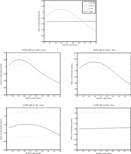
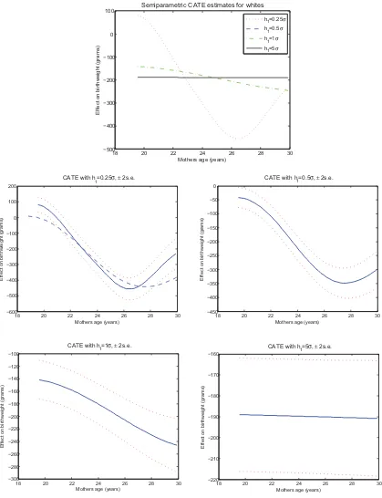
Our benchmark estimates are depicted inFigure 2(blacks) andFigure 3(whites). We report four different CATE estimates corresponding to bandwidthsh1=0.25 ˆσ ,0.5 ˆσ ,1 ˆσ ,5 ˆσ, where
ˆ
σ is the sample standard deviation ofX1 (mother’s age). In
both figures the top panel shows the four estimates together; the bottom panels show them separately along with±2 standard errors. Ash1increases, the estimated CATE functions become
flatter, less variable, and their range shrinks. The CATE estimate corresponding to the smallest value ofh1actually shows a
posi-tive and somewhat significant smoking effect around age 19–20 for both races; increasing the bandwidth causes this anomaly to disappear. While more smoothing might guard against CATE estimates with unreasonable values, it also goes against the gen-eral philosophy of the exercise—to let the data speak about the heterogeneity of the smoking effect with as mild restrictions as possible. Indeed, forh1=5 ˆσ, the estimates are only
informa-tive about the overall average effect, estimated to be about−155 grams for blacks and−190 for whites.
Taken globally, all the nonconstant CATE estimators tell a similar story—the predicted average effect of smoking, by and large, becomes stronger (more negative) at higher ages. For blacks, this monotone relationship is possibly broken by a hump around age 19–20, and for whites by a “check mark” shape in the late 20s. However, these features become less pronounced with more smoothing. The overall negative slope is consistent with the results obtained by Walker, Tekin, and Wallace (2009), who reported OLS and matching estimates that are more negative for adult mothers than for teen mothers. The advantage of our approach over simple and somewhat arbitrary sample splitting is that CATE is potentially capable of delivering a more detailed picture of age-related heterogeneity. A natural but speculative explanation for the results is that age is positively correlated with how long an individual has smoked, and long-term smok-ing has a cumulative negative effect on birth weight. Another possibility is that the correlation between smoking and other unobserved harmful behaviors that are not picked up by our controls becomes stronger with age.
For a given age, the numerical values of the CATE point estimates can vary substantially withh1. For example, for blacks
at age 26 the estimated effect ranges from about −150 g to −480 g, a factor of 3. Similarly, if we consider, say, whites at age 20, we again see differences in point estimates on the order of 300 g, despite the fact that the estimated confidence intervals do not suggest such large sampling variation. Again,
17 18 19 20 21 22 23 24 25 26 −500
−400 −300 −200 −100 0 100 200
Semiparametric CATE estimates for blacks
Mother’s age (years)
Effect on birthweight (grams)
h
1=0.25σ
h
1=0.5σ
h
1=1σ
h1=5σ
17 18 19 20 21 22 23 24 25 26 −800
−600 −400 −200 0 200 400
CATE with h
1=0.25σ,± 2s.e.
Mother’s age (years)
Effect on birthweight (grams)
17 18 19 20 21 22 23 24 25 26 −500
−400 −300 −200 −100 0 100 200
CATE with h1=0.5σ,± 2s.e.
Mother’s age (years)
Effect on birthweight (grams)
17 18 19 20 21 22 23 24 25 26 −250
−200 −150 −100 −50 0
CATE with h
1=1σ,± 2s.e.
Mother’s age (years)
Effect on birthweight (grams)
17 18 19 20 21 22 23 24 25 26 −240
−220 −200 −180 −160 −140 −120 −100 −80
CATE with h1=5σ,± 2s.e.
Mother’s age (years)
Effect on birthweight (grams)
Figure 2. Baseline estimates of CATE (mother’s age) for blacks.
this underscores the need for sensitivity analysis and data-driven procedures to guide bandwidth choice in finite samples.
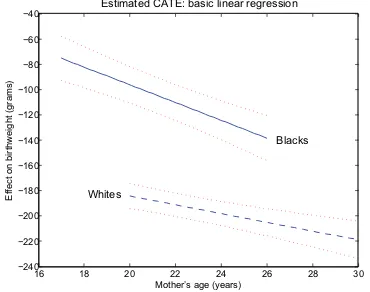
We perform a number of robustness checks in addition to varyingh1. First, we estimate CATE using the linear regression
method proposed in Section 2.2; the results are displayed in Figure 4. Consistent with the overall shape of the semiparamet-ric estimates, the regression-based CATE functions also have a negative slope. In fact, while a bit steeper, the semiparamet-ric estimates forh1=1×σˆ are reasonably close to the OLS
estimates for both groups.
Regarding the sufficiency of our controls, the level differences in the estimates for blacks versus whites could be interpreted as evidence that confounding factors are not completely accounted for by the conditioning variables (we are grateful to a referee
for pointing this out). Nevertheless, it is not straightforward to pinpoint the omitted factors. A potential concern could be the decline in smoking incidence during the sample period (or that it might have taken place differently among the two groups). However, adding “year fixed effects” (i.e., birth year) toXdoes not change the baseline results in a noteworthy way. As the North Carolina vital statistics include the mother’s zip code, we can link some zip-code level characteristics, such as annual mean income, to individuals. Adding such controls does not appreciably change the results either.
Varying the point at which the propensity score estimates are trimmed has a more substantial effect. For example, setting
α=2% implies dropping only 4% of observations for whites and 6.5% for blacks. The general shape of the estimated CATE