Full Terms & Conditions of access and use can be found at
http://www.tandfonline.com/action/journalInformation?journalCode=ubes20
Download by: [Universitas Maritim Raja Ali Haji] Date: 11 January 2016, At: 22:56
Journal of Business & Economic Statistics
ISSN: 0735-0015 (Print) 1537-2707 (Online) Journal homepage: http://www.tandfonline.com/loi/ubes20
Bias-Corrected Matching Estimators for Average
Treatment Effects
Alberto Abadie & Guido W. Imbens
To cite this article: Alberto Abadie & Guido W. Imbens (2011) Bias-Corrected Matching
Estimators for Average Treatment Effects, Journal of Business & Economic Statistics, 29:1, 1-11, DOI: 10.1198/jbes.2009.07333
To link to this article: http://dx.doi.org/10.1198/jbes.2009.07333
Published online: 01 Jan 2012.
Submit your article to this journal
Article views: 764
View related articles
Bias-Corrected Matching Estimators for
Average Treatment Effects
Alberto A
BADIEJohn F. Kennedy School of Government, Harvard University, Cambridge, MA 02138 and NBER (alberto_abadie@harvard.edu)
Guido W. I
MBENSDepartment of Economics, Harvard University, Cambridge, MA 02138 and NBER (imbens@harvard.edu)
In Abadie and Imbens (2006), it was shown that simple nearest-neighbor matching estimators include a conditional bias term that converges to zero at a rate that may be slower thanN1/2. As a result, match-ing estimators are notN1/2-consistent in general. In this article, we propose a bias correction that ren-ders matching estimatorsN1/2-consistent and asymptotically normal. To demonstrate the methods pro-posed in this article, we apply them to the National Supported Work (NSW) data, originally analyzed in Lalonde (1986). We also carry out a small simulation study based on the NSW example. In this simula-tion study, a simple implementasimula-tion of the bias-corrected matching estimator performs well compared to both simple matching estimators and to regression estimators in terms of bias, root-mean-squared-error, and coverage rates. Software to compute the estimators proposed in this article is available on the au-thors’ web pages (http:// www.economics.harvard.edu/ faculty/ imbens/ software.html) and documented in Abadie et al. (2003).
KEY WORDS: Selection on observables; Treatment effects.
1. INTRODUCTION
The purpose of this article is to investigate the properties of estimators that combine matching with a bias correction pro-posed in Rubin (1973) and Quade (1982), and derive the large sample properties of a nonparametric extension of the bias-corrected estimator. We show that a nonparametric implemen-tation of the bias correction removes the conditional bias of matching asymptotically to a sufficient degree so that the re-sulting estimator is N1/2-consistent, without affecting the as-ymptotic variance.
We apply simple matching estimators and the bias-corrected matching estimators studied in the current article to the Na-tional Supported Work (NSW) demonstration data, analyzed originally by Lalonde (1986) and subsequently by many oth-ers, including Heckman and Hotz (1989), Dehejia and Wahba (1999), Smith and Todd (2005), and Imbens (2003). For the Lalonde dataset we show that conventional matching estima-tors without bias correction are sensitive to the choice for the number of matches, whereas a simple implementation of the bias correction using linear least squares is relatively robust to this choice. Moreover, in small simulation studies designed to mimic the data from the NSW application, we find that the simple linear least-squares based implementation of the bias-corrected matching estimator performs well compared to both matching estimators without bias correction, and to regression and weighting estimators, in terms of bias, root-mean-squared-error, and coverage rates for the associated confidence intervals. Bias-corrected matching estimators combine some of the ad-vantages and disadad-vantages of both matching and regression estimators. Compared to matching estimators without bias cor-rection, they have the advantage of beingN1/2-consistent and asymptotically normal irrespective of the number of covariates. However, bias-corrected matching estimators may be more dif-ficult to implement than matching estimators without bias cor-rection if the bias corcor-rection is calculated using nonparametric
smoothing techniques, and therefore, involves the choice of a smoothing parameter as a function of the sample size. Com-pared to estimators based on nonparametric regression adjust-ment without matching (e.g., Hahn1998; Heckman et al.1998; Imbens, Newey, and Ridder 2005; Chen, Hong, and Tarozzi 2008) or weighting estimators (Horvitz and Thompson 1952; Robins and Rotnitzky1995; Hirano, Imbens, and Ridder2003; Abadie2005), bias-corrected matching estimators have the ad-vantage of an additional layer of robustness because matching ensures consistency for any given value of the smoothing para-meters without requiring accurate approximations to either the regression function or the propensity score. However, in con-trast to some regression adjustment and weighting estimators, bias-corrected matching estimator have the disadvantage of not being fully efficient (Abadie and Imbens2006).
2. MATCHING ESTIMATORS
2.1 Setting and Notation
Matching estimators are often used in evaluation research to estimate treatment effects in the absence of experimental data. As is by now common in this literature, we use Rubin’s po-tential outcome framework (e.g., Rubin1974). See Rosenbaum (1995) and Imbens and Wooldridge (2009) for surveys. ForN units, indexed byi=1, . . . ,N, letWibe a binary variable that indicates exposure of individualito treatment, so thatWi=1 if individualiwas exposed to treatment, andWi=0 otherwise. LetN0=Ni=1(1−Wi)andN1=Ni=1Wi=N−N0be the number of control and treated units, respectively. The variables Yi(0)andYi(1)represent potential outcomes with and without
© 2011American Statistical Association Journal of Business & Economic Statistics
January 2011, Vol. 29, No. 1 DOI:10.1198/jbes.2009.07333
1
treatment, respectively, and therefore,Yi(1)−Yi(0)is the treat-ment effect for uniti. Depending on the value ofWi, one of the two potential outcomes is realized and observed:
Yi=
Yi(0) ifWi=0 Yi(1) ifWi=1.
In settings with essentially unrestricted heterogeneity in the ef-fect of the treatment, the typical goal of evaluation research is to estimate an average treatment effect. Here, we focus on the unconditional (population) average
τ=E[Yi(1)−Yi(0)].
In addition, in the applied literature the focus is often on the average effect for the treated,
τtreated=E[Yi(1)−Yi(0)|Wi=1].
In the body of the article we will largely focus onτ. In Appen-dix Bwe present the corresponding results forτtreated.
In general, a simple comparison of average outcomes be-tween treated and control units does not identify the average effect of the treatment. The reason is that this comparison may be contaminated by the effect of other variables that are cor-related with the treatment, Wi, as well as with the potential outcomes,Yi(1)andYi(0). The presence of these confounders may create a correlation between Wi andYi even if the treat-ment has no causal effect on the outcome. Randomization of the treatment eliminates the correlation between any potential confounder andWi. In the absence of randomization, the fol-lowing set of assumptions has been found useful as a basis for identification and estimation ofτ when all confounders are ob-served. These observed confounders for unitiwill be denoted byXi, a vector of dimensionk, withjth elementXij.
Assumption A.1. LetX be a random vector of dimension k of continuous covariates distributed onRk with compact and convex supportX, with (a version of the) density bounded and bounded away from zero on its support.
Assumption A.2. For almost everyx∈X,
(i) (unconfoundedness)W is independent of(Yi(0),Yi(1)) conditional onXi=x;
(ii) (overlap) η <Pr(Wi =1|Xi =x) < 1−η, for some
η >0.
Assumption A.3. {(Yi,Wi,Xi)}Ni=1 are independent draws from the distribution of(Y,W,X).
Assumption A.4. Letμw(x)=E[Yi(w)|Xi=x]andσw2(x)=
E[(Yi−μw(x))2|Xi=x]. Then, (i)μw(x)and σw2(x)are Lip-schitz inXforw=0,1, (ii)E[(Yi(w))4|Xi=x] ≤Cfor some finiteC, for almost allx∈X, and (iii)σw2(x)is bounded away from zero.
AssumptionA.1requires that all variables inX have a con-tinuous distribution. Notice, however, that discrete covariates with a finite number of support points can be easily accommo-dated in our analysis by conditioning on their values. Assump-tionA.2(i) states that, conditional onXi, the treatmentWiis “as good as randomized,” that is, it is independent of the potential outcomes,Yi(1)andYi(0). That will be the case, in particular, if all potential confounders are included inX. Therefore, con-ditional onXi=x, a simple comparison of average outcomes
between treated and control units is equal to the average effect of the treatment givenXi =x. This assumption originates in the seminal article by Rosenbaum and Rubin (1983). Assump-tionA.2(ii) is the usual support condition invoked for matching estimators. Assumption A.2(i) and Assumption A.2(ii) com-bined are referred to as “strong ignorability.” AssumptionA.3 refers to the sampling process. Finally, AssumptionA.4collects regularity conditions that will be used later. Note that given As-sumptionA.2(i),μw(x)=E[Yi|Xi=x,Wi=w], andσw2(x)=
E[(Yi−E[Yi|Xi=x,Wi=w])2|Xi=x,Wi=w]. Abadie and Imbens (2006) discussed Assumptions A.1 through A.4 in greater detail. Identification conditions for matching estimators are also discussed in Hahn (1998), Dehejia and Wahba (1999), Lechner (2002), and Imbens (2004), among others.
As in Abadie and Imbens (2006), we consider matching “with replacement,” allowing each unit to be used as a match more than once. Forx∈X, and for some positive definite sym-metric matrix A, let xA=(x′Ax)1/2 be some vector norm. Typically the k×k matrix A is choosen to be the inverse of the sample covariance matrix of the covariates, corresponding to the Mahalanobis metric,
Amaha=
1 N
N
i=1
(Xi−X)·(Xi−X)′
−1
,
whereX= 1 N
N
i=1 Xi,
or the normalized Euclidean distance, the diagonal matrix with the inverse of the sample variances on the diagonal (e.g., Abadie and Imbens2006):
Ane=diag(A−maha1 )− 1.
Letℓm(i)be the index of themth match to uniti. That is, among the units in the opposite treatment group to uniti, unitℓm(i)is themth closest unit to unitiin terms of covariate values. Thus, ℓm(j)satisfies, (i)Wℓm(i)=1−Wi, and (ii)
j:Wj=1−Wi
1
Xj−XiA≤
Xℓm(i)−Xi
A =m,
where1{·} is the indicator function, equal to 1 if the expres-sion in brackets is true and zero otherwise. For notational sim-plicity, we ignore ties in the matching, which happen with probability zero if the covariates are continuous. LetJM(i)=
{ℓ1(i), . . . , ℓM(i)} denote the set of indices for the first M matches for uniti, for M such thatM≤N0 andM≤N1. Fi-nally, letKM(i)denote the number of times unitiis used as a match if we match each unit to the nearestMmatches:
KM(i)= N
l=1
1{i∈JM(l)}.
Under matching without replacement,Km(i)∈ {0,1}, but in our setting of matching with replacement,Km(i)can also take on integer values larger than 1 if unit i is the closest match for multiple units.
2.2 Estimators
If we were to observe the potential outcomes Yi(0) and Yi(1) for all units, we will simply estimate τ as the average
N
i=1(Yi(1)−Yi(0))/N. The idea behind matching estimators is to estimate, for eachi=1, . . . ,N, the missing potential out-comes. For each i we know one of the potential outcomes, namelyYi(0)ifWi=0, andYi(1)otherwise. Hence, ifWi=0, then we choose Yˆi(0)=Yi(0)=Yi, and if Wi=1, then we chooseYˆi(1)=Yi(1)=Yi. The remaining potential outcome for unitiis imputed using the average of the outcomes for its matches. This leads to
Using this notation, we can write the matching estimators forτ based onMmatches per unit, with replacement, as
ˆ
Using the definition ofKM(i), we can also write this estimator as a weighted average of the outcomes,
ˆ
This representation is useful for deriving the variance of the matching estimator.
In empirical applications, matching estimators are often im-plemented with small values for M, as small as 1 even in reasonably large sample sizes. Therefore, in order to obtain an accurate approximation to the finite sample distribution of matching estimators in such settings, we focus asymptotic ap-proximations asNincreases for fixedM.
Before introducing the bias-corrected matching estimator, let us briefly discuss regression estimators. Letμˆw(x)be a consis-tent estimator ofμw(x). A regression imputation estimator uses
ˆ
the regression imputation estimator ofτ is
ˆ
As in Abadie and Imbens (2006), we classify as regression im-putation estimators those for which μˆw(x)is a consistent es-timator ofμw(x). Various forms of such estimators were pro-posed by Hahn (1998), Heckman et al. (1998), Chen, Hong, and Tarozzi (2008), and Imbens, Newey, and Ridder (2005).
The matching estimators in Equation (1) are similar to the re-gression imputation estimators, as they can be interpreted as imputing Yi(0)andYi(1) with a nearest-neighbor estimate of
μ0(Xi)andμ1(Xi), respectively. However, because M is held fixed under the matching asymptotics, Yˆi(0)andYˆi(1)do not estimateμ0(Xi)andμ1(Xi)consistently.
Finally, we consider a bias-corrected matching estimator where the difference within the matches is regression-adjusted for the difference in covariate values:
˜
Rubin (1979) and Quade (1982) discussed such estimators in the context of matching without replacement and with linear covariance adjustment.
To further illustrate the difference between the simple match-ing estimator, the regression estimator, and the bias-corrected matching estimator, consider unitiwithWi=0. For this unit, Yi(0)is known, and onlyYi(1)needs to be imputed. The sim-ple matching estimator imputes the missing potential outcome Yi(1)as
The regression imputation estimator imputes this missing po-tential outcome as
Yi(1)= ˆμ1(Xi).
The bias-corrected matching estimator imputes the missing po-tential outcome as
The imputation for the bias-corrected matching estimator ad-justs the imputation under the simple matching estimator by the difference in the estimated regression function at Xi and the estimated regression function at the matched values,Xjfor j∈JM(i). Obviously that will improve the estimator if the es-timated regression function is a good approximation to the true regression function. Even if the estimated regression function is noisy, the adjustment will typically be small becauseXi−Xjfor j∈JM(i)should be small in large samples. At the same time,
compared to the regression estimator, the bias-corrected match-ing estimator adds M1
j∈JM(i)Yj(1)− ˆμ1(Xj). If the estimated
regression function is equal to the true regression function, this is simply adding noise to the estimator, making it less precise without introducing bias. However, if the regression function is misspecified, the fact that under very weak assumptions the ex-pectation of M1
j∈JM(i)Yj(1)converges toμ1(Xi)implies that
bias correction, relative to imputation estimators, is, in expecta-tion, approximately equal toμ1(Xi)− ˆμ1(Xi), which will elim-inate any inconsistency in the regression imputation estimator. In other words, the bias-corrected matching estimator is robust against misspecification of the regression function.
2.3 Large Sample Properties of Matching Estimators
Before presenting some results on the large sample properties of the bias-corrected matching estimator, we first collect some results on the large sample properties of matching estimators derived in Abadie and Imbens (2006), which motivated the use of bias-corrected matching estimators.
First, we introduce some additional notation. LetX be the N×kmatrix withith row equal toX′i. Similarly, letWbeN×1 vector withith element equal toWi. Let
τ (x)=E[Yi(1)−Yi(0)|Xi=x] =μ1(x)−μ0(x),
be the average effect of the treatment conditional onX=x, and
τ (X)= 1
the average of that over the covariate distribution. For i= 1, . . . ,N, define
Now we can write the simple matching estimator minus the av-erage treatment effect using simple algebra as
ˆ tional treatment effect. This term is a simple sample average and satisfies a central limit theorem. The second termDN has expectation zero conditional onXandW. This term also sat-isfies a central limit theorem (Abadie and Imbens2006). The last term captures the bias conditional on the covariates. This
term does not necessarily satisfy a central limit theorem, and our bias-correction approach is geared toward eliminating it.
Next, we turn to the variance. Note thatKM(i)is nonstochas-tic conditional on XandW. Therefore, Equation (2) implies that the variance ofτˆMmconditional onXandWis ing result is given in Abadie and Imbens (2006):
Theorem 1(Asymptotic normality for the simple matching estimator). Suppose AssumptionsA.1–A.4hold. Then
VE+Vτ (X)−1/2√
N(τˆMm−BmM−τ )−→d N(0,1).
Abadie and Imbens (2006) also proposed a consistent esti-mator forVEandVτ (X)under AssumptionsA.1–A.4.
The result of Theorem1shows that, after subtracting the con-ditional bias termsBmM, the simple matching estimator isN1/2 -consistent and asymptotically normal. Moreover, Abadie and Imbens (2006) showed that the same result holds without sub-tracting the conditional bias terms if matching is done for only one covariate (e.g., matching on the true propensity score) be-cause in that case√NBmM=op(1).
3. BIAS CORRECTED MATCHING
In this section we analyze the properties of the bias-corrected matching estimators, defined in Equation (3). In order to estab-lish the asymptotic behavior of the bias-corrected estimator, we consider a nonparametric series estimator for the two regres-sion functions,μ0(x)andμ1(x), withK(N)terms in the series, whereK(N)increases with N. An important disadvantage of this estimator is that it will rely on selecting smoothing para-meters as functions of the sample size, something that the sim-ple matching estimator allows us to avoid. The advantage of the bias-corrected matching estimator is that it is root-Nconsistent for any dimension of the covariates,k. In both these properties the bias-corrected matching estimator is similar to the regres-sion imputation estimator. However, it has the same large sam-ple variance as the simsam-ple matching estimator, and therefore, it is, in general, not as efficient as the regression imputation or weighting estimators in large samples. Compared to the regres-sion imputation estimator, the bias-corrected matching estima-tor is more robust in the sense that it is consistent for a fixed value of the smoothing parameters. Because choosing smooth-ing parameters as functions of the sample size is precisely what matching estimators allow us to avoid, in the empirical analy-sis and simulations of Sections4and5we investigate the per-formance of a simple implementation of the bias correction by linear least squares.
Here, we discuss the formal nonparametric implementation of the bias adjustment. Letλ=(λ1, . . . , λk)be a multi-index of dimensionk, that is, ak-dimensional vector of nonnegative integers, with |λ| =k
i=1λi, and let xλ =xλ11, . . . ,xλkk. Con-sider a series {λ(K)}∞K=1 containing all distinct such vectors such that|λ(K)| is nondecreasing. LetpK(x)=xλ(K), and let
pK(x)=(p1(x), . . . ,pK(x))′. Following Newey (1995), the non-parametric series estimator of the regression functionμw(x)is given by
ˆ
μw(x)=pK(N)(x)′
i:Wi=w
pK(N)(Xi)pK(N)(Xi)′
−
×
i:Wi=w
pK(N)(Xi)Yi,
where(·)−denotes a generalized inverse. Given the estimated regression function, letBˆmMbe the estimator for the average bias term:
ˆ
BmM= 1 N
N
i=1
2Wi−1 M
M
j=1
ˆ
μ1−Wi(Xi)− ˆμ1−Wi
Xℓj(i)
.
Then the bias corrected matching estimator is
ˆ
τMbcm= ˆτMm− ˆBmM. (4)
The following theorem shows that the bias correction removes the bias without affecting the asymptotic variance.
Theorem 2 (Bias-corrected matching estimator). Suppose that AssumptionsA.1–A.4hold. Assume also that (i) the sup-port ofX,X⊂Rk, is a Cartesian product of compact intervals; (ii)K(N)=O(Nν), with 0< ν <min(2/(4k+3),2/(4k2−k)); and (iii) there is a constantCsuch that for each multi-indexλ the λth partial derivative ofμw(x)exists forw=0,1 and its norm is bounded byC|λ|. Then,
√
N(BmM− ˆBmM)−→p 0 and
VE+Vτ (X)1/2√
N(τˆMbcm−τ )−→d N(0,1).
Proof. SeeAppendix A.
The first result implies that we can estimate the bias faster thanN1/2. This may seem surprising, given that even in para-metric settings we can typically not estimate parameters faster than N1/2. That logic applies to objects of the type μw(x)−
μw(z); for fixed xand w we cannot estimateμw(x)−μw(z) faster than N1/2. However, here we are estimating objects of the typeμw(x)−μw(z)wherez−xgoes to zero, allowing us to obtain a faster rate for the differenceμw(x)−μw(z). In other words,BmM itself isop(1)[in fact, it isOp(N−1/k), giving us ad-ditional room to estimate it at a rate faster thanN1/2]. The sec-ond result says that the bias-corrected matching estimator has the same normalized variance as the simple matching estimator.
4. AN APPLICATION TO THE EVALUATION OF A
LABOR MARKET PROGRAM
In this section we apply the estimators studied in this arti-cle to data from the National Supported Work (NSW) demon-stration, an evaluation of a subsidized work program first an-alyzed by Lalonde (1986) and subsequently by Heckman and Hotz (1989), Dehejia and Wahba (1999), Imbens (2003), Smith and Todd (2005), and others. The specific sample we use here is the one employed by Dehejia and Wahba (1999) and is avail-able on Rajeev Dehejia’s website. The dataset we use here con-tains an experimental sample from a randomized evaluation of the NSW program, and also a nonexperimental sample from the Panel Study of Income Dynamics (PSID). Using the experimen-tal data we obtain an unbiased estimate of the average effect of the program. We then compute nonexperimental matching esti-mators using the experimental participants and the nonexperi-mental comparison group from the PSID, and compare them to the experimental estimate. In line with previous studies using these data, we focus on the average effect for the treated, and therefore, only match the treated units.
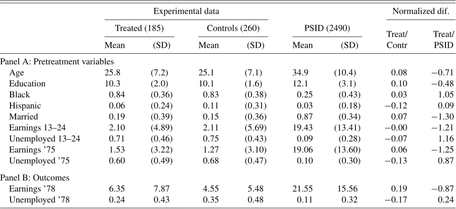
Table1presents summary statistics for the three groups used in our analysis. The first two columns present the summary
sta-Table 1. Summary statistics
Experimental data Normalized dif.
Treated (185) Controls (260) PSID (2490)
Treat/ Treat/
Mean (SD) Mean (SD) Mean (SD) Contr PSID
Panel A: Pretreatment variables
Age 25.8 (7.2) 25.1 (7.1) 34.9 (10.4) 0.08 −0.71 Education 10.3 (2.0) 10.1 (1.6) 12.1 (3.1) 0.10 −0.48 Black 0.84 (0.36) 0.83 (0.38) 0.25 (0.43) 0.03 1.05 Hispanic 0.06 (0.24) 0.11 (0.31) 0.03 (0.18) −0.12 0.09 Married 0.19 (0.39) 0.15 (0.36) 0.87 (0.34) 0.07 −1.30 Earnings 13–24 2.10 (4.89) 2.11 (5.69) 19.43 (13.41) −0.00 −1.21 Unemployed 13–24 0.71 (0.46) 0.75 (0.43) 0.09 (0.28) −0.07 1.16 Earnings ’75 1.53 (3.22) 1.27 (3.10) 19.06 (13.60) 0.06 −1.25 Unemployed ’75 0.60 (0.49) 0.68 (0.47) 0.10 (0.30) −0.13 0.87
Panel B: Outcomes
Earnings ’78 6.35 7.87 4.55 5.48 21.55 15.56 0.19 −0.87 Unemployed ’78 0.24 0.43 0.35 0.48 0.11 0.32 −0.17 0.24
NOTE: Earnings data are in thousands of 1978 dollars. Earnings 13–24 and Unemployed 13–24 refers to earnings and unemployment during the period 13 to 24 months prior to randomization.
tistics for the experimental treatment group. The second pair of columns presents summary statistics for the experimental controls. The third pair of columns presents summary statistics for the nonexperimental comparison group constructed from the PSID. The last two columns present normalized differences between the covariate distributions, between the experimental treated and controls, and between the experimental treated and the PSID comparison group, respectively. These normalized differences are calculated as
nor-dif=X1−X0
(S20+S21)/2 ,
where Xw =i:Wi=wXi/Nw and S
2 w=
i:Wi=w(Xi−Xw)
2/
(Nw−1). Note that this differs from thet-statistic for the test of the null hypothesis thatE[X|W=0] =E[X|W=1], which will be
t-stat= X1−X0
S20/N0+S21/N1 .
The normalized difference provides a scale-free measure of the difference in the location of the two distributions, and is useful for assessing the degree of difficulty in adjusting for differences in covariates.
Panel A contains the results for pretreatment variables and Panel B for outcomes. Notice the large differences in back-ground characteristics between the program participants and the PSID sample. This is what makes drawing causal inferences
from comparisons between the PSID sample and the treatment group a tenuous task. From Panel B, we can obtain an unbi-ased estimate of the effect of the NSW program on earnings in 1978 by comparing the averages for the experimental treated and controls, 6.35−4.55=1.80, with a standard error of 0.67 (earnings are measured in thousands of dollars). Using a nor-mal approximation to the limiting distribution of the effect of the program on earnings in 1978, we obtain a 95% confidence interval, which is[0.49,3.10].
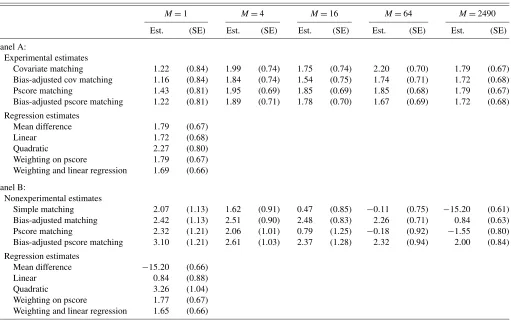
Table2presents estimates of the causal effect of the NSW program on earnings using various matching, regression, and weighting estimators. Panel A reports estimates for the exper-imental data (treated and controls). Panel B reports estimates based on the experimental treated and the PSID comparison group. The first set of rows in each case reports matching es-timates forM equal to 1, 4, 16, 64, and 2490 (the size of the PSID comparison group). The matching estimates include sim-ple matching with no-bias adjustment and bias-adjusted match-ing, first by matching on the covariates and then by matching on the estimated propensity score. The covariate matching es-timators use the matrixAne(the diagional matrix with inverse sample variances on the diagonal) as the distance measure. Be-cause we are focused on the average effect for the treated, the bias correction only requires an estimate ofμ0(Xi). We esti-mate this regression function using linear regression on all nine pretreatment covariates in Table1, panel A, but do not include any higher order terms or interactions, with only the control units that are used as a match [the unitsjsuch thatWj=0 and
Table 2. Experimental and nonexperimental estimates for the NSW data
M=1 M=4 M=16 M=64 M=2490
Est. (SE) Est. (SE) Est. (SE) Est. (SE) Est. (SE)
Panel A:
Experimental estimates
Covariate matching 1.22 (0.84) 1.99 (0.74) 1.75 (0.74) 2.20 (0.70) 1.79 (0.67) Bias-adjusted cov matching 1.16 (0.84) 1.84 (0.74) 1.54 (0.75) 1.74 (0.71) 1.72 (0.68) Pscore matching 1.43 (0.81) 1.95 (0.69) 1.85 (0.69) 1.85 (0.68) 1.79 (0.67) Bias-adjusted pscore matching 1.22 (0.81) 1.89 (0.71) 1.78 (0.70) 1.67 (0.69) 1.72 (0.68)
Regression estimates
Mean difference 1.79 (0.67)
Linear 1.72 (0.68)
Quadratic 2.27 (0.80)
Weighting on pscore 1.79 (0.67) Weighting and linear regression 1.69 (0.66)
Panel B:
Nonexperimental estimates
Simple matching 2.07 (1.13) 1.62 (0.91) 0.47 (0.85) −0.11 (0.75) −15.20 (0.61) Bias-adjusted matching 2.42 (1.13) 2.51 (0.90) 2.48 (0.83) 2.26 (0.71) 0.84 (0.63) Pscore matching 2.32 (1.21) 2.06 (1.01) 0.79 (1.25) −0.18 (0.92) −1.55 (0.80) Bias-adjusted pscore matching 3.10 (1.21) 2.61 (1.03) 2.37 (1.28) 2.32 (0.94) 2.00 (0.84)
Regression estimates
Mean difference −15.20 (0.66)
Linear 0.84 (0.88)
Quadratic 3.26 (1.04)
Weighting on pscore 1.77 (0.67) Weighting and linear regression 1.65 (0.66)
NOTE: The outcome is earnings in 1978 in thousands of dollars.
j∈JM(i)for somei]. The confidence intervals are based on the variance estimator proposed in Abadie and Imbens (2006). This variance estimator is formally justified for the case of matching on the covariates. It does not cover the case of matching on the estimated propensity score. We implement it for the case of matching on the estimated propensity score by ignoring the estimation error in the propensity score. The next three rows of each panel report estimates based on differences in means, linear regression including terms for all covariates, and linear regression also including quadratic terms and a full set of in-teractions, respectively. The last two rows in each panel report estimates for weighting estimators. Both rows use weights for the treated units equal to 1, and weights for the control units equal to the propensity score divided by 1 minus the propen-sity score. Then we normalize the weights in both groups to add up toN1. The first weighting estimator is based solely on weighting, the second one uses weighted regression, with the nine pretreatment variables included.
The experimental estimates in Panel A range from 1.16 (bias-corrected matching with one match) to 2.27 (quadratic re-gression). The nonexperimental estimates in Panel B have a much wider range, from −15.20 (simple difference) to 3.26 (quadratic regression). For the nonexperimental sample, us-ing a sus-ingle match, there is little difference between the sim-ple matching estimator and its bias-corrected version, 2.07 and 2.42, respectively. However, simple matching without bias-correction produces radically different estimates when the num-ber of matches changes; a troubling result for the empirical implementation of these estimators. WithM≥16, the simple matching estimator produces results outside the experimental 95% confidence interval. In contrast, the bias-corrected match-ing estimator shows a much more robust behavior when the number of matches changes: only withM=2490 (that is, when all units in the comparison group are matched to each treated) the bias-corrected estimate deteriorates to 0.84, still inside the experimental 95% confidence interval.
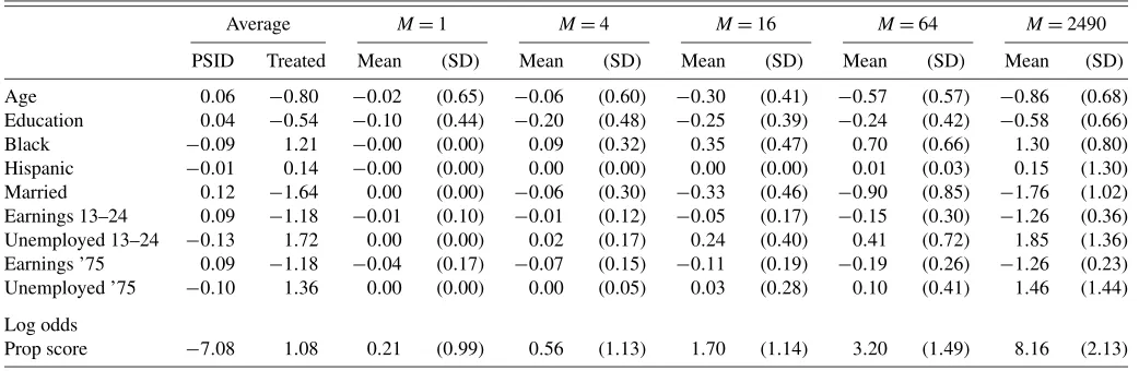
To see how well the simple matching estimator performs in terms of balancing the covariates, Table3reports average dif-ferences within the matched pairs. First, all the covariates are normalized to have zero mean and unit variance. The first two
columns report the averages of the normalized covariates for the PSID comparison group and the experimental treated. Before matching, the averages for some of the variables are more than one standard deviation apart, e.g., the earnings and employ-ment variables. The next pair of columns reports the within-matched-pairs average difference and the standard deviation of this within-pair difference. For all the indicator variables the matching is exact. The other, more continuously distributed variables are not matched exactly, but the quality of the matches appears very high: the average difference within the pairs is very small compared to the average difference between treated and comparison units before the matching, and it is also small compared to the standard deviations of these differences. If we increase the number of matches the quality of the matches goes down, with even the indicator variables no longer matched ex-actly, but in most cases the average difference is still very small until we get to 16 or more matches. As expected, match quality deteriorates when the number of matches increases. This ex-plains why, as shown in Table 2, the bias correction matters more for larger M. The last row reports matching differences for logistic estimates of the propensity score. Although here we match on the covariates directly, rather than on the propen-sity score, the matching still greatly reduces differences in the propensity score. With a single match (M=1) the average dif-ference in the propensity score is only 0.21, whereas without matching the difference between treated and comparison units is 8.16, almost 40 times higher.
5. A MONTE CARLO STUDY
In this section, we discuss some simulations designed to as-sess the performance of the various matching estimators. To get a realistic sense of the performance of the various estima-tors, we simulated datasets that aim to resemble actual datasets. For other Monte Carlo studies of matching type estimators see Zhao (2002), Frölich (2004), and Busso, DiNardo, and McCra-ry (2009). An additional Monte Carlo study based on data col-lected by Imbens, Rubin, and Sacerdote (2001) is available in a previous version of this article.
Table 3. Mean covariate differences in matched groups
Average M=1 M=4 M=16 M=64 M=2490
PSID Treated Mean (SD) Mean (SD) Mean (SD) Mean (SD) Mean (SD)
Age 0.06 −0.80 −0.02 (0.65) −0.06 (0.60) −0.30 (0.41) −0.57 (0.57) −0.86 (0.68) Education 0.04 −0.54 −0.10 (0.44) −0.20 (0.48) −0.25 (0.39) −0.24 (0.42) −0.58 (0.66) Black −0.09 1.21 −0.00 (0.00) 0.09 (0.32) 0.35 (0.47) 0.70 (0.66) 1.30 (0.80) Hispanic −0.01 0.14 −0.00 (0.00) 0.00 (0.00) 0.00 (0.00) 0.01 (0.03) 0.15 (1.30) Married 0.12 −1.64 0.00 (0.00) −0.06 (0.30) −0.33 (0.46) −0.90 (0.85) −1.76 (1.02) Earnings 13–24 0.09 −1.18 −0.01 (0.10) −0.01 (0.12) −0.05 (0.17) −0.15 (0.30) −1.26 (0.36) Unemployed 13–24 −0.13 1.72 0.00 (0.00) 0.02 (0.17) 0.24 (0.40) 0.41 (0.72) 1.85 (1.36) Earnings ’75 0.09 −1.18 −0.04 (0.17) −0.07 (0.15) −0.11 (0.19) −0.19 (0.26) −1.26 (0.23) Unemployed ’75 −0.10 1.36 0.00 (0.00) 0.00 (0.05) 0.03 (0.28) 0.10 (0.41) 1.46 (1.44)
Log odds
Prop score −7.08 1.08 0.21 (0.99) 0.56 (1.13) 1.70 (1.14) 3.20 (1.49) 8.16 (2.13)
NOTE: In this table all covariates have been normalized to have mean zero and unit variance. The first two columns present the averages for the experimental treated and the PSID comparison units. The remaining pairs of columns present the average difference within the matched pairs and the standard deviation of this difference for matching based on 1, 4, 16, 64, and 2490 matches. For the last variable the logarithm of the odds ratio of the propensity score is used. This log odds ratio has mean−6.52 and standard deviation 3.30 in the sample.
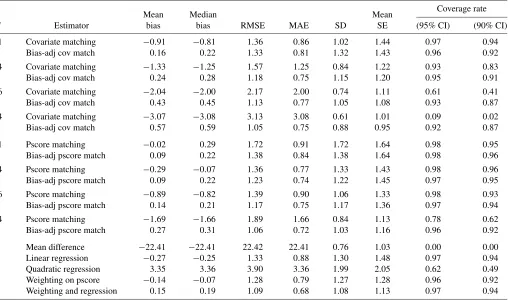
Table 4. Simulation results Lalonde design (10,000 replications)
Coverage rate
Mean Median Mean
M Estimator bias bias RMSE MAE SD SE (95% CI) (90% CI)
1 Covariate matching −0.91 −0.81 1.36 0.86 1.02 1.44 0.97 0.94 Bias-adj cov match 0.16 0.22 1.33 0.81 1.32 1.43 0.96 0.92
4 Covariate matching −1.33 −1.25 1.57 1.25 0.84 1.22 0.93 0.83 Bias-adj cov match 0.24 0.28 1.18 0.75 1.15 1.20 0.95 0.91
16 Covariate matching −2.04 −2.00 2.17 2.00 0.74 1.11 0.61 0.41 Bias-adj cov match 0.43 0.45 1.13 0.77 1.05 1.08 0.93 0.87
64 Covariate matching −3.07 −3.08 3.13 3.08 0.61 1.01 0.09 0.02 Bias-adj cov match 0.57 0.59 1.05 0.75 0.88 0.95 0.92 0.87
1 Pscore matching −0.02 0.29 1.72 0.91 1.72 1.64 0.98 0.95 Bias-adj pscore match 0.09 0.22 1.38 0.84 1.38 1.64 0.98 0.96 4 Pscore matching −0.29 −0.07 1.36 0.77 1.33 1.43 0.98 0.96 Bias-adj pscore match 0.09 0.22 1.23 0.74 1.22 1.45 0.97 0.95
16 Pscore matching −0.89 −0.82 1.39 0.90 1.06 1.33 0.98 0.93 Bias-adj pscore match 0.14 0.21 1.17 0.75 1.17 1.36 0.97 0.94
64 Pscore matching −1.69 −1.66 1.89 1.66 0.84 1.13 0.78 0.62 Bias-adj pscore match 0.27 0.31 1.06 0.72 1.03 1.16 0.96 0.92
Mean difference −22.41 −22.41 22.42 22.41 0.76 1.03 0.00 0.00 Linear regression −0.27 −0.25 1.33 0.88 1.30 1.48 0.97 0.94 Quadratic regression 3.35 3.36 3.90 3.36 1.99 2.05 0.62 0.49 Weighting on pscore −0.14 −0.07 1.28 0.79 1.27 1.28 0.96 0.92 Weighting and regression 0.15 0.19 1.09 0.68 1.08 1.13 0.97 0.94
The simulations are designed to mimic the Lalonde data. In each of the 10,000 replications we draw 185 treated and 2490 control observations and calculate 21 estimators for the average effect on the treated,τtreated. In the simulation we have eight regressors, designed to match the following variables in the NSW dataset: age,educ, black, married,re74, u74, re75, and u75. InAppendix Cwe describe the precise data generating process for the simulations. For each estimator we report the mean and median bias, the root-mean-squared-error (RMSE), the median-absolute-error (MAE), the standard devi-ation, the average estimated standard error, and the coverage rates for nominal 95% and 90% confidence intervals based on the matching estimator for the variance. We implemented an ex-tremely simple version of the bias adjustment, using only linear terms in the covariates. The results are reported in Table4.
In terms of RMSE and MAE, the bias-adjusted matching es-timator is best with 64 matches, but with this many matches the bias is substantial. With four matches the bias is considerably smaller, and the actual coverage rates of the 90% and 95% con-fidence intervals is close to the nominal coverage rate. The sim-ple (not bias-adjusted) matching estimator does not perform as well, in terms of bias or RMSE. The pure regression adjustment estimators perform poorly. They have high RMSE and substan-tial bias. Coverage rates of confidence intervals centered on the bias-corrected matching estimator are closer to nominal levels than those centered on the simple matching estimator. Confi-dence intervals for the quadratic regression estimator have sub-stantially lower than nominal coverage rates, although coverage rates for the linear regression estimator are close to the nomi-nal rates. In this setting the weighting estimators do fairly well, both in terms of coverage rates and in terms of RMSE.
6. CONCLUSION
We propose a nonparametric bias-adjustment that renders matching estimators N1/2-consistent. In simulations based on a realistic setting for nonexperimental program evaluations, a simple implementation of this estimator, where the bias-adjustment is based on linear regression, performs well com-pared to both matching estimators without bias-adjustment and regression-based estimators in terms of bias and mean-squared error. It also has good coverage rates for 90% and 95% confi-dence intervals, suggesting it may be a useful estimator in prac-tice.
APPENDIX A: PROOFS
Before proving Theorem 2 we state two auxiliary lem-mas. Let λ be a multi-index of dimension k, that is, a k -dimensional vector of nonnegative integers, with|λ| =k
i=1λi, and letl be the set ofλ such that |λ| =l. Furthermore, let xλ=xλ1
1 , . . . ,x λk
k , and let∂ λg(x)
=∂|λ|g(x)/∂xλ1
1 , . . . , ∂x λk
k . For d≥0, define|g|d=max|λ≤d|supx|∂λg(x)|.
Lemma A.1(Uniform convergence of series estimators of re-gression functions, Newey 1995). Suppose the conditions in Theorem2hold. Then for anyξ >0 and nonnegative integerd,
| ˆμw−μw|d=OpK1+2d(K/N)1/2+K−ξ forw=0,1.
Proof. Assumptions 3.1, 4.1, 4.2, and 4.3 in Newey (1995) are satisfied forμw(x)andNw→ ∞, implying that Newey’s theorems 4.2 and 4.4 apply. The result of the lemma holds be-causeN/Nw=Op(1)forw=0,1.
Lemma A.2(Unit-level bias correction). Suppose the condi-tions in Theorem2hold. Then
max
aroundXito write
formly bounded, applying Bonferroni’s and Markov’s inequali-ties, we obtain that for anyε >0: Because we can chooseε≤1/2, it follows that the left-hand side of the last equation isop(N−1/2). Similarly, for anyε >0:
Therefore, for arbitraryξ >0 andε >0:
max
We focus on the result for the average treatment effect. The second part of the theorem for the average effect for the treated follows the same pattern. The difference| ˆBmM−BmM|can be
writ-APPENDIX B: THE AVERAGE EFFECT ON THE TREATED
Here we present the results for the average effect on the treated without proof. The formal proofs are similar to those for the case of the overall average effect. Estimation ofτtreated requires weaker assumptions than estimation ofτ. In particular, AssumptionsA.2andA.3can be weakened as follows.
Assumption A.2′. For almost everyx∈X,
(i) Wis independent ofY(0)conditional onX=x; (ii) Pr(W=1|X=x) <1−η, for someη >0.
Assumption A.3′. Conditional onWi=wthe sample consists of independent draws fromY,X|W=w, forw=0,1. For some r≥1,N1r/N0→θ, with 0< θ <∞.
Using the same definition forYˆi(0)as before, we now esti-mateτtreatedandτcond,treatedas
ˆ
the estimator for the average bias
ˆ
the bias-corrected estimator for the average effect on the treated
ˆ
τMbcm,treated= ˆτMm,treated− ˆBmM,treated,
the conditional variance
V(τˆMm,treated|X,W)
= 1
N12 N
i=1
Wi−(1−Wi) KM(i)
M
2
σ2(Xi,Wi),
and its normalized version,
VtreatedE =N1·V(τˆMm,treated|X,W).
Also define Vtreatedτ (X) =E[(τ (X)−τtreated)2|W =1]. Then the equivalent of Theorems1and2is:
Theorem 1′ (Asymptotic normality for the simple matching estimator for the average effect on the treated). Suppose As-sumptionsA.1,A.2′,A.3′, andA.4hold. Then
VtreatedE +Vtreatedτ (X) −1/2
N1
×(τˆMm,treated−BmM,treated−τtreated) d
−→N(0,1). Theorem 2′ (Bias-corrected matching estimator for the av-erage effect on treated). Suppose that AssumptionsA.1,A.2′, A.3′, andA.4hold. Assume also that (i) the support ofX,X⊂ Rk, is a Cartesian product of compact intervals; (ii) K(N)= O(Nν), with 0 < ν < min(2/(4k+ 3),2/(4k2 − k)); and (iii) there is a constantCsuch that for each multi-indexλthe λth partial derivative ofμw(x)exists forw=0,1 and its norm is bounded byC|λ|. Then,
N1(BmM,treated− ˆBmM,treated) p
−→0
and
VtreatedE +Vtreatedτ (X) 1/2N1(τˆMbcm,treated−τtreated) d
−→N(0,1).
APPENDIX C: DATA GENERATING PROCESSES FOR THE SIMULATIONS
(i) Covariates. We draw separately from the covariate dis-tribution givenWi=0 andWi=1. The covariates are grouped into a set of five subsets, and between the subsets the covariates are drawn independently. The groups of covariates are{age},
{educ}, {black}, {married}, and {u74,u75,re74,
re75}. For each of the joint distributions within a subset the distribution follows fairly closely to the corresponding distrib-ution in the Lalonde data.
Among the control observations, the log ofagehas a nor-mal distribution with mean 3.50 and standard deviation 0.30. Among the treated it has a normal distribution with mean 3.22 and standard deviation 0.25.
educhas a discrete distribution with points of support of all integers between 4 and 16. The probabilities for the 13 points of support for the controls are 0.02, 0.01, 0.02, 0.02, 0.06, 0.04, 0.07, 0.07, 0.34, 0.05, 0.08, 0.02, and 0.20. For the treated the probabilities are 0.02, 0.01, 0.01, 0.01, 0.10, 0.15, 0.17, 0.24, 0.21, 0.04, 0.02, 0.01, and 0.01.
blackhas a discrete distribution with, among the controls,
the population fraction of blacks is 0.25. Among the treated the fraction is 0.84.
Among the controls,marriedhas a binary distribution with mean 0.87, and among the treated it has a binary distribution with mean 0.19.
Among the controls the pr((u74,u75)=(0,0))=0.88, pr((u74,u75)=(0,1))=0.03 pr((u74,u75)=(1,0)) = 0.02, and pr((u74,u75)=(1,1))=0.07. Among the treated pr((u74,u75)=(0,0))=0.28, pr((u74,u75)=(0,1)) = 0.01, pr((u74,u75)=(1,0))=0.12, and pr((u74,u75)= (1,1))=0.59.
Among the controls, conditional on(u74,u75)=(0,1), the log ofre75has a normal distribution with mean 2.32 and stan-dard deviation 1.45, conditional on (u74,u75)=(1,0), the log ofre74has a normal distribution with mean 2.16 and stan-dard deviation 1.20, and conditional on (u74,u75)=(0,0), the log of(re74,re75)has a joint normal distribution with mean(2.88,2.86)and covariance matrix0.37000.47 0.50000.37 .
Among the treated, conditional on(u74,u75)=(0,1), the log of re75 has a normal distribution with mean 0.60 and standard deviation 0.88, conditional on (u74,u75)=(1,0), the log ofre74has a normal distribution with mean 1.26 and variance 0.78, and conditional on(u74,u75)=(0,0), the log of (re74,re75) has a joint normal distribution with mean (1.53,0.93)and covariance matrix1.080.57 0.571.42.
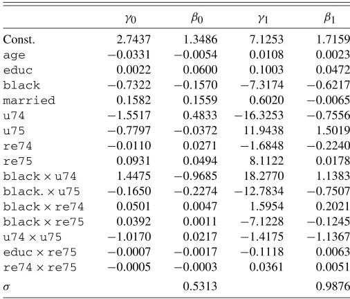
(ii) Conditional Outcome Distribution Given Covariates. Conditional on the covariates, the outcome Yi has a mixed discrete/continuous distribution, with separate coefficients for the controls and treated. The probability that the outcome is positive conditional on the covariate taking on the value x is exp(γw′h(x))/(1+exp(γw′h(x)), for w=0,1. The vector of covariates contains 16 elements: an intercept,age,educ,
black,married,u74,u75,re74,re75,black×u74,
black×u75,black×re74,black×re75,u75×u74,
educ×re75, and re74×re75. The coefficients γ are listed in Table C.1. Conditional on the outcome being posi-tive, its logarithm has a normal distribution with meanβw′h(x),
Table C.1. Data generating process for Lalonde simulations
γ0 β0 γ1 β1
Const. 2.7437 1.3486 7.1253 1.7159
age −0.0331 −0.0054 0.0108 0.0023
educ 0.0022 0.0600 0.1003 0.0472
black −0.7322 −0.1570 −7.3174 −0.6217
married 0.1582 0.1559 0.6020 −0.0065
u74 −1.5517 0.4833 −16.3253 −0.7556
u75 −0.7797 −0.0372 11.9438 1.5019
re74 −0.0110 0.0271 −1.6848 −0.2240
re75 0.0931 0.0494 8.1122 0.0178
black×u74 1.4475 −0.9685 18.2770 1.1383
black.×u75 −0.1650 −0.2274 −12.7834 −0.7507
black×re74 0.0501 0.0047 1.5954 0.2021
black×re75 0.0392 0.0011 −7.1228 −0.1245
u74×u75 −1.0170 0.0217 −1.4175 −1.1367
educ×re75 −0.0007 −0.0017 −0.1118 0.0063
re74×re75 −0.0005 −0.0003 0.0361 0.0051
σ 0.5313 0.9876
forw=0,1, and varianceσ2, for the same vector of functions of the covariates h(x). Again the values for βw are given in TableC.1.
ACKNOWLEDGMENTS
The authors thank the financial support for this research, gen-erously provided through NSF grants SES-0350645 (Abadie), SBR-0452590, and SBR-0820361 (Imbens). A previous ver-sion of this article circulated under the title “Simple and Bias-Corrected Matching Estimators for Average Treatment Effects” (Abadie and Imbens2002).
[Received December 2007. Revised August 2009.]
REFERENCES
Abadie, A. (2005), “Semiparametric Difference-in-Differences Estimators,” Review of Economic Studies, 72, 1–19. [1]
Abadie, A., and Imbens, G. (2002), “Simple and Bias-Corrected Matching Es-timators for Average Treatment Effects,” Technical Working Paper T0283, NBER. [11]
(2006), “Large Sample Properties of Matching Estimators for Average Treatment Effects,”Econometrica, 74 (1), 235–267. [1-4,7]
Abadie, A., Drukker, D., Herr, H., and Imbens, G. (2003), “Implementing Matching Estimators for Average Treatment Effects in STATA,”The Stata Journal, 4 (3), 290–311.
Busso, M., DiNardo, J., and McCrary, J. (2009), “New Evidence on the Finite Sample Properties of Propensity Score Matching and Reweighting Estima-tors,” unpublished manuscript, Dept. of Economics, UC Berkeley. [7] Chen, X., Hong, H., and Tarozzi, A. (2008), “Semiparametric Efficiency in
GMM Models of Nonclassical Measurement Errors,”The Annals of Sta-tistics, 36 (2), 808–843. [1,3]
Dehejia, R., and Wahba, S. (1999), “Causal Effects in Nonexperimental Studies: Reevaluating the Evaluation of Training Programs,”Journal of the Ameri-can Statistical Association, 94, 1053–1062. [1,2,5]
Frölich, M. (2004), “Finite Sample Properties of Propensity-Score Matching and Weighting Estimators,”Review of Economics and Statistics, 86 (1), 77– 90. [7]
Hahn, J. (1998), “On the Role of the Propensity Score in Efficient Semipara-metric Estimation of Average Treatment Effects,”Econometrica, 66 (2), 315–331. [1-3]
Heckman, J., and Hotz, J. (1989), “Choosing Among Alternative Nonexperi-mental Methods for Estimating the Impact of Social Programs: The Case of Manpower Training” (with discussion),Journal of the American Statistical Association, 84, 862–874. [1,5]
Heckman, J., Ichimura, H., Smith, J., and Todd, P. (1998), “Characterizing Selection Bias Using Experimental Data,”Econometrica, 66, 1017–1098. [1,3]
Hirano, K., Imbens, G., and Ridder, G. (2003), “Efficient Estimation of Average Treatment Effects Using the Estimated Propensity Score,”Econometrica, 71, 1161–1189. [1]
Horvitz, D., and Thompson, D. (1952), “A Generalization of Sampling Without Replacement From a Finite Universe,”Journal of the American Statistical Association, 47, 663–685. [1]
Imbens, G. (2003), “Sensitivity to Exogeneity Assumptions in Program Evalu-ation,”American Economic Review Papers and Proceedings, 93 (2), 126– 132. [1,5]
(2004), “Nonparametric Estimation of Average Treatment Effects Un-der Exogeneity: A Review,”Review of Economics and Statistics, 86, 4–30. [2]
Imbens, G. W., and Wooldridge, J. (2009), “Recent Developments in the Econo-metrics of Program Evaluation,”Journal of Economic Literature, 47, 5–86. [1]
Imbens, G., Newey, W., and Ridder, G. (2005), “Mean-Squared-Error Calcu-lations for Average Treatment Effects,” unpublished manuscript, Harvard University, Dept. of Economics. [1,3]
Imbens, G., Rubin, D., and Sacerdote, B. (2001), “Estimating the Effect of Un-earned Income on Labor Supply, Earnings, Savings and Consumption: Evi-dence From a Survey of Lottery Players,”American Economic Review, 91, 778–794. [7]
Lalonde, R. J. (1986), “Evaluating the Econometric Evaluations of Training Programs With Experimental Data,”American Economic Review, 76, 604– 620. [1,5]
Lechner, M. (2002), “Some Practical Issues in the Evaluation of Heterogeneous Labour Market Programmes by Matching Methods,”Journal of the Royal Statistical Society, Ser. A, 165, 59–82. [2]
Newey, W. (1995), “Convergence Rates for Series Estimators,” inStatistical Methods of Economics and Quantitative Economics: Essays in Honor of C. R. Rao(eds. G. S. Maddala, P. C. B. Phillips, and T. N. Srinavasan), Cambridge: Blackwell. [5,8]
Quade, D. (1982), “Nonparametric Analysis of Covariance by Matching,” Bio-metrics, 38, 597–611. [1,3]
Robins, J., and Rotnitzky, A. (1995), “Semiparametric Efficiency in Multivari-ate Regression Models With Missing Data,”Journal of the American Sta-tistical Association, 90, 122–129. [1]
Rosenbaum, P. (1995),Observational Studies, New York: Springer-Verlag. [1] Rosenbaum, P., and Rubin, D. (1983), “The Central Role of the Propensity Score in Observational Studies for Causal Effects,”Biometrika, 70, 41–55. [2]
Rubin, D. (1973), “The Use of Matched Sampling and Regression Adjustments to Remove Bias in Observational Studies,”Biometrics, 29, 185–203. [1]
(1974), “Estimating Causal Effects of Treatments in Randomized and Nonrandomized Studies,”Journal of Educational Psychology, 66, 688–701. [1]
(1979), “Using Multivariate Matched Sampling and Regression Ad-justment to Control Bias in Observational Studies,”Journal of the American Statistical Association, 74, 318–328. [3]
Smith, J., and Todd, P. (2005), “Does Matching Address LaLonde’s Critique of Nonexperimental Estimators,”Journal of Econometrics, 125, 305–353. [1,5]
Zhao, Z. (2002), “Using Matching to Estimate Treatment Effects: Data Require-ments, Matching Metrics and an Application,” unpublished manuscript, Dept. of Economics, Johns Hopkins University. [7]