Full Terms & Conditions of access and use can be found at
http://www.tandfonline.com/action/journalInformation?journalCode=ubes20
Download by: [Universitas Maritim Raja Ali Haji] Date: 12 January 2016, At: 01:06
Journal of Business & Economic Statistics
ISSN: 0735-0015 (Print) 1537-2707 (Online) Journal homepage: http://www.tandfonline.com/loi/ubes20
Statistical Inference with Generalized Gini Indices
of Inequality, Poverty, and Welfare
Garry F. Barrett & Stephen G. Donald
To cite this article: Garry F. Barrett & Stephen G. Donald (2009) Statistical Inference with Generalized Gini Indices of Inequality, Poverty, and Welfare, Journal of Business & Economic Statistics, 27:1, 1-17, DOI: 10.1198/jbes.2009.0001
To link to this article: http://dx.doi.org/10.1198/jbes.2009.0001
Published online: 01 Jan 2012.
Submit your article to this journal
Article views: 173
Statistical Inference with Generalized Gini
Indices of Inequality, Poverty, and Welfare
Garry F. B
ARRETTSchool of Economics, University of New South Wales, Sydney, NSW, 2052 (g.barrett@unsw.edu.au)
Stephen G. D
ONALDDepartment of Economics, University of Texas at Austin, Austin, TX, 78712 (donald@eco.utexas.edu)
This article considers statistical inference for consistent estimators of generalized Gini indices of in-equality, poverty, and welfare. Our method does not require grouping the population into a fixed number of quantiles. The empirical indices are shown to be asymptotically normally distributed using functional limit theory. Easily computed asymptotic variance expressions are obtained using influence functions. Inference based on first-order asymptotics is then compared with the grouped method and various bootstrap methods in simulations and with U.S. income data. The bootstrap-tmethod based on our asymptotic theory is found to have superior size and power properties in small samples.
KEY WORDS: Functional delta method; Generalized Gini index; Influence function.
1. INTRODUCTION
The work of Atkinson (1970), Kolm (1969), and Sen (1973) generated new interest in the theory of inequality measurement. Their contributions emphasized the duality between measures of inequality (and poverty) and welfare, and led to a large lit-erature proposing new indices of inequality explicitly derived from the desired properties of the underlying social welfare function (SWF) (see Lambert 1993 for an in depth survey). More recently, researchers have begun examining the statistical properties of these normative measures of inequality and poverty so that they can be used for formal statistical inference. A key development was the work of Beach and Davidson (1983), who presented the variance-covariance matrix of a vector of Lorenz curve (LC) ordinates without placing para-metric restrictions on the form of the underlying income dis-tribution. Subsequently, researchers have used the results in Beach and Davidson to derive the sampling distribution of the Gini-type inequality (Barrett and Pendakur 1995; Rongve and Beach 1997; Davidson and Duclos 1997) and welfare indices (Bishop, Chakraborti, and Thistle 1990) and poverty measures (Xu and Osberg 1998), which can be expressed as functions of LC ordinates or income quantiles. In a related strand of work, Cowell (1989) and Thistle (1990) derived the large sample distribution of the Atkinson and generalized entropy indices, which are functions of the raw moments of a distribution.
A fundamental limitation of the current approach to deriving the sampling distribution of the Gini indices is that the indices are expressed as a function of a small, finite number of LC ordinates rather than the complete set of ordinates implied by an empirical distribution function. Consequently, the estima-tors of the indices are inconsistent. By considering only a small number of ordinates, inequality within population quantiles is ignored and an underestimate of the true level of inequality is obtained. The inconsistency is greater the greater is the level of aggregation into quantiles (the smaller the set of ordinates) and the more unequal is the underlying income distribution. This research embodies a compromise between using a desirable measure of inequality and being able to undertake formal statistical inference.
Important exceptions are the work of Cowell (1989) on the traditional Gini coefficient and Bishop, Formby, and Zheng (1997) and Xu (2006) on the ‘‘Sen poverty indices,’’ who use results from the theory of U-statistics to derive the sampling properties of consistent estimators of these indices. Zitikis and Gastwirth (2002) and Zitikis (2003) consider an alternative approach to the asymptotics of Gini inequality indices from that pursued in Barrett and Donald (2000)—an earlier draft of this article. Xu (2000) proposed a bootstrap method for testing differences in the generalized Gini relative indices of inequality. Since the Gini indices are not asymptotically piv-otal, Xu (2000) considered a bias corrected, iterative variant of the bootstrap. In this article, we derive asymptotic results using influence functions that generalize the results derived by Cowell (1989), Bishop et al. (1997), Zitikis and Gastwirth (2002), and Zitikis (2003) to all members of the generalized Gini class of inequality, poverty, and welfare indices.
In this article, we examine the asymptotic distribution of a variety of inequality, poverty, and welfare measures that can be written as statistical functionals of either the LC or generalized Lorenz curve (GLC). We use results concerning the delta method for statistical functionals to derive the asymptotic properties of the generalized Gini indices. Our approach to estimating standard errors, constructing confidence intervals (CIs), and performing inference is, like that of Beach and Davidson (1983), nonparametric since we impose no structure on the underlying income distribution beyond weak regularity conditions. Our approach to inference differs from that of Beach and Davidson (1983) in that we use the influence functions for the various objects. The use of the influence function to study the statistical properties of estimators was pioneered by Hampel (1974), and one of the first applications in econometrics was by Cowell and Victoria-Feser (1996), who examined the sensitivity of summary measures of inequality to data contamination. As a by-product of our approach, we
2009 American Statistical Association Journal of Business & Economic Statistics January 2009, Vol. 27, No. 1 DOI 10.1198/jbes.2009.0001 1
provide an alternative means for computing the variance-covariance matrix for a vector of LC and GLC ordinates. The influence function approach has considerable computational advantages for obtaining consistent estimates of the asymptotic variances of the Gini-based indices. Further, our approach does not require the aggregation of the population in a small set of Lorenz ordinates for the computation of the indices. Our asymptotic results show that the desirable normative properties of quantile-based inequality, poverty, and welfare indices need not be compromised to undertake inferential analysis. We compare inference procedures based on our asymptotic results, including the bootstrap-t method, with those for the grouped Gini estimator and a variety of alternative bootstrap procedures in a series of Monte Carlo experiments and in an empirical application. The simple asymptotic methods are found to per-form well, while, in line with theory, the bootstrap-t method, which uses the asymptotic variance estimator to form a pivotal test statistic, is found to have superior performance in small samples.
The article is organized as follows. The next section briefly reviews the set of inequality, poverty, and welfare indices that can be written as functionals of the LC or GLC. In Section 3, the sampling distribution of these measures is derived. Section 4 briefly summarizes the alternative approaches to inference with the Gini indices based on asymptotic and bootstrap resampling methods. The alternative approaches are compared in a series of Monte Carlo experiments and their relative per-formance evaluated. In Section 5, the methods are illustrated by examining changes in income inequality and poverty in the United States between 1988 and 1998. Concluding comments are provided in the final section.
2. MEASURES OF INEQUALITY AND POVERTY
2.1 Preliminaries
The objective is to undertake statistical inference with the normative indices of inequality and poverty, which are gen-eralizations of the Gini coefficient. Let Y denote the ran-dom variable income, and let the population CDF be given byF(y), which is assumed to be continuous and differentiable to at least second order. Also let Q(p) ¼ F1(p) denote the pth quantile of income. The LC for the distribution is then given by
LðpÞ ¼ 1
m
Z QðpÞ
0
y:dFðyÞ
¼ 1
m
Z p
0
QðtÞdt;
ð1Þ
wheremis the mean level of income. The LC represents the proportion of total income going to the bottompproportion of the population. Closely related to the LC is the GLC,
GðpÞ ¼pEðYjY #QðpÞÞ
¼
Z QðpÞ
0
y:dFðyÞ
¼
Z p
0 QðtÞdt
ð2Þ
which is often used for welfare comparisons when income distributions have unequal means (Shorrocks 1983). These curves are popular tools in the literature on inequality and welfare measurement, and, as shown subsequently, a variety of indices of inequality and poverty can be represented as func-tionals of either the GLC or the LC.
2.2 S-Gini Indices
The S-Gini relative indices of inequality are given by
IdR¼1dðd1Þ
Z 1
0 ð
1pÞd2LðpÞdðpÞ; ð3Þ
where 1 <d < ‘. The index is scale free (homogeneous of degree 0 in y) and S-Concave (Blackorby and Donaldson, 1978). The ‘‘inequality aversion parameter’’ d is set by the researcher. Higher values of d place progressively greater social weight on transfers involving individuals ranked toward the bottom of the distribution. The special case ofd¼2 cor-responds to the popular Gini coefficient. A fuller discussion of the properties of the S-Gini indices are given in Donaldson and Weymark (1980, 1983), Kakwani (1980), and Yitzhaki (1983).
The S-Gini absolute index of inequality is given by
IdA ¼mdðd1Þ
Z 1
0 ð
1pÞd2GðpÞdp: ð4Þ
Absolute inequality indices are a function of absolute income differentials rather than income shares and have been inter-preted as measures of relative deprivation (Yitzhaki 1979).
The S-Gini inequality indices imply, and are implied by, the same class of ordinally equivalent social welfare functions (SWFs). The welfare index underlying the S-Gini inequality indices can be represented in two ways using integration by parts and (2)
Wd¼dðd1Þ
Z 1
0 ð
1pÞd2GðpÞdp¼d
Z 1
0 ð
1pÞd1QðpÞdp
ð5Þ with the second being useful from the standpoint of computa-tion (Seccomputa-tion 3). It is easy to see that once one has obtained the welfare index, the inequality indexes can be found using IdA ¼mWd andIdR ¼ ðmWdÞ=m: The special case ofWd whend ¼2 corresponds to the Sen welfare index. The sam-pling distribution of this particular index was analyzed by Bishop et al. (1990): the results presented in Section 3.3 gen-eralize their result to consistent estimators of all members (1 <
d<‘) of the Gini family of welfare indices.
2.3 E-Gini Indices
Another set of generalized Gini indices are the E-Ginis presented by Chakravarty (1988). The E-Gini relative index is
IaR¼2
Z 1
0 ð
pLðpÞÞadp
a1
; ð6Þ
where a $ 1 is the inequality aversion parameter. As a
increases, the index is increasingly sensitive to transfers at the lower end of the income distribution. Whena¼1, the index
corresponds to the Gini coefficient, and asa!‘, the index approaches twice the Schutz index (the maximum distance between the LC and line of equality).
The key normative distinction between the S-Gini and E-Gini indices is that only the E-E-Ginis (for a > 1) satisfy the ‘‘principle of diminishing transfers.’’ The S-Ginis are linear in incomes, and the social weight attached to individuals is a function of their rank in the ordered distribution. The effect of a transfer on the level of measured inequality will be a function of the ranks of the individuals involved in the transfer. How-ever, the E-Ginis are a CES function of the difference between the LC and the line of equality, and the effect of a transfer on measured inequality will be sensitive to the differences in individuals’ income shares (see Chakravarty, 1988, for a proof and fuller discussion).
The E-Gini absolute index of inequality is given by
IaA ¼2
Underlying the E-Gini relative and absolute inequality indices is a common class of SWFs. One cardinalization of the E-Gini welfare index is
Conceptually, Wa represents the level of income, which, if distributed equally to all members of the population, generates the same level of social welfare as the actual distribution. The welfare index is equal to (twice) the mean scaled down by the level of inequality.
2.4 Gini Poverty Indices
Indices of poverty are closely related to measures of inequality and welfare (Sen 1976). Following Blackorby and Donaldson (1980), normative poverty indices can be expressed as a composite function of the proportion of the population below the poverty line (the head-count ratio), the average income of the poor, and the level of income inequality among the poor:
wherezis the income level representing the ‘‘poverty line,’’ IR(y|y<z) is the level of relative inequality among the poor, and
m(z) is the average income of the poor. Equivalently, the gen-eralized Gini poverty indices can be expressed as a composite function of the proportion of the population below the poverty line (F(z)) and the normalized Gini welfare indices defined over the poorW(y|z).
The S-Gini welfare index defined over the poor is given by
WdðyjzÞ ¼ 1
when d ¼ 1, where 1(A) represents the indicator function, which is equal to 1 when A is true (and 0 otherwise). Con-sequently, using (9), (10), and (11), the S-Gini poverty index is
Pd¼FðzÞ 1 equal to the head-count ratio times the average income shortfall of the poor divided by the poverty line. This particular index can be simply estimated using a scaled average, making esti-mation and inference straightforward. Whend¼2,Pd corre-sponds to the well-known Sen index of poverty; the sampling distribution of this specific index was analyzed by Bishop et al. (1997) and Xu (2006).
When the welfare index underlying the E-Gini indices is adopted, the conditional social welfare of the poor is given by
Wa¼2 mðzÞ 1 and, hence, the E-Gini poverty-based index is defined as
Pa ¼FðzÞ 1 parameterizes the aversion to income inequality among the poor.
3. VARIANCE ESTIMATION FOR THE EMPIRICAL GENERALIZED GINI ESTIMATORS
3.1 Definition of Empirical Indices
Our basic approach uses the property that all of the indices described previously are functionals of the LC or GLC and the CDF at a particular point in the case of the poverty indices, and we can consistently estimate these functionals by plugging in empirical versions of the LC, GLC, and CDF. We assume that we have a random samplefYig
N
i¼1 drawn from an underlying distribution with CDFF(y). We assume thatF:[yl,yu]![0, 1], where (i) 0 <yl< yu< ‘, (ii)Fis twice continuously differ-entiable with densityf(y)¼F9(y), and (iii) 0 < infyf(y) < supy f(y) <‘. The discussion of the empirical estimators and their asymptotic standard errors in this section assumes an iid random sample for simplicity. It is straightforward to allow for independent but non-identically distributed samples by constructing consistent, weighted estimates of the components, which form the indices and the variances (Cameron and
Trivedi 2005). Indeed, most survey datasets used in dis-tributional analysis, including the Current Population Survey (CPS) data used in Section 5, are weighted samples, where the weights often represent the inverse probability of selection from the population. It is also possible to allow for more complex sampling schemes in the estimation of the Gini indices and asymptotic variances using the framework pre-sented in Bhattacharya (2005). Biewen (2002) outlines how bootstrap procedures may be adapted to replicate complex or dependent sampling schemes to produce interval estimates and hypothesis tests.
For the S-Gini indices, we have that
^ LCs, respectively. Given the definitions in (1) and (2), these can be computed according to the ‘‘analogy principle’’ (Manski 1988) as
QðtÞis the empirical quantile of the distribution ofYiand can be defined as
^
QðpÞ ¼inffy: ^FðyÞ$ pg;
where F^ðyÞ is the empirical distribution for the sample de-fined by
For the E-Gini indices, we have
^
while the Gini-based poverty indices can be written as
^
In this section, we consider the issue of computing the estimates of the inequality indices. A technical appendix to the article, which is available on each author’s webpage, details how one can compute the influence curves for all of the indices considered in the article. Given our treatment of the indices as statistical functionals of the GLC or LC, it is instructive to first consider the computation of the GLC and LC. Denote the ordered, distinct sample values for theYiby the notationyjso that
yl#y1 < y2 < < yN_ # yu;
where N_ is the number of distinct values in the sample with N_< N if there are ties in the sample. The
esti-occurring at each of theyjvalues. Therefore, the estimatorF^ðyÞ takes on the valuePj
l¼1p^j¼p^j on the interval [yj,yjþ1). We
can then define the quantile function using similar arguments. In terms of theyj, the quantile estimator is
^
Given the preceding representation, it is straightforward to calculate the integrals that define the GLC and LC. In partic-ular, forpsuch thatp2 ½p^j1;p^jÞ, we have simplicity, we assume thatyN_ ¼yuso that by construction for p¼1 we have
which is the sample mean of theYi. Given the estimator of the GLC, it is then straightforward to see that
^
LðpÞ ¼G^ðpÞ ^ Gð1Þ;
which is how we have defined our LC estimator previously. Note thatG^ð0Þ ¼L^ð0Þ ¼0 andL^ð1Þ ¼1:The LC estimate is also piecewise linear and continuous on [0, 1].
In computing the S-Gini indices, it is most convenient to use the representation in terms of quantiles. Use is made of the fact that
Z 1
where the relevant functions have been defined over the intervalsðp^j1;p^j:Using the result in (5) we can estimate the S-Gini indices using the empirical quantiles, which gives an alternative way of calculatingW^dby
^
Then using (16)–(18) we can compute the S-Gini-based indices as follows:
Next, for the E-Gini indices, it is necessary to calculate the quantity
so that the general integral does not apply. With these calcu-lations, we can then compute the indices by
^
Computation of the Gini poverty indices is very similar to that for the Gini inequality indices. The computation ofP^d in the case whered> 1 andP^aonly will be considered, since the case ofP^dwithd¼1 is a simple average. For the S-Gini-based index we can use a similar result to (5) to show that the expression in (24) is equivalent to
^
where the second line follows after a change of variables. To estimate this quantity, we defineN(z) to be the value for which
^
FðzÞ ¼pNðzÞ, which is the number of observations that are less than or equal to the poverty linez. Then, similar to the esti-mation of the S-Gini inequality indices, we can compute the poverty index by
Similar arguments for the E-Gini-based index suggest esti-mating the index in the form
^
where, using a change of variable and arguments similar to those used to deriveT^E,
3.3 Asymptotic Variance Estimation Using Influence Functions
All of the objects defined previously, such as those in (16)– (18) and (21)–(26), can be written in the following general form:
^
T ¼c1^u1þc2^u2þTðH^Þ;
where cj are scalar constants, ^uj are scalar estimators, and where TðH^Þ is a scalar valued functional of some process
^
Hthat is defined on [0, 1]. For instance, in the case of the S-Gini, the absolute inequality index c1^u1 is given by m^, H^ is given by the empirical generalized LCG^ðpÞ, and the functional Tis given by
TðHÞ ¼ dðd1Þ
Z 1
0 ð
1pÞd2HðpÞdp: ð27Þ
The relevant scalar estimators for the other indexes areF^ðzÞ andG^ðF^ðzÞÞ. The additional relevant processes areL^ðpÞ,p
^
LðpÞ, m^pG^ðpÞ, G^ðpF^ðzÞÞ, and pG^ðF^ðzÞÞ G^ðpF^ðzÞÞ. Fi-nally, the other relevant functionals are 2½R1
0HðpÞ a
dpa1 and scaled versions of this and the functional in (27).
There are two important elements in the derivation of the variances. First, it is the case that for the scalars we can write influence function and give the effect of an observation on the estimator. In many estimation problems, thefið^ujÞare iid with finite variance. Thus, the first term on the right-hand side of (28) satisfies a central limit theorem and implies that the asymptotic variance of the estimator is equal to the expectation of the squared influence function. Hence, the asymptotic var-iance of the estimator can be estimated by taking the sample average of the squared influence functions. For example, the influence function for the estimatorF^ðyÞis given by
fiðy;FÞ ¼1ðYi #yÞ FðyÞ;
Due to the fact that thefi(y;F) are iid mean zero with variance given by
Eðfiðy;FÞ 2
Þ ¼FðyÞð1FðyÞÞ;
one can estimate the asymptotic variance of ffiffiffiffi
N p
ðF^ðyÞ FðyÞÞ and the standard error ofF^ðyÞby using, respectively,
^ function. In addition to their use in variance estimation, influence functions have also been used in the study of robust statistics (Reid, 2005).
Given that the influence functionfið^ujÞterms in (28) are iid and satisfy a central limit theorem, it follows that
ffiffiffiffi
N p
ð^ujujÞ !d Nð0;Eðf
iðujÞ2Þ: ð29Þ The expression in (28) also follows easily form^, since
ffiffiffiffi method for scalars. The form of the expression in (28) and the result in (29) leads to a natural estimator of the asymp-totic variance in (29) by taking the average off^
ið^ujÞ2, where ^
fið^ujÞis an estimate offið^ujÞ.
The second key element in our derivation of asymptotic variances for the indices is to extend the ideas in the previous paragraph to functionals TðH^Þ in general. Specifically, we show the steps in deriving a similar expansion to (28) for the termTðH^Þ, whereH^is now a function. We assume that
ffiffiffiffi
N p
ðH^HÞ0H ð30Þ
for some Gaussian processHon [0, 1] that takes its values in a function spaceH0and that there exists an expansion such as in
(28) for each pointp2[0, 1] so that wherefiðp; ^HÞare the iid influence functions. An implication of this is that
ffiffiffiffi
To derive similar results for the functionalTðH^Þ, we appeal to a version of the Delta methods that is appropriate for functionals and requires that the functionalTis Hadamard differentiable at F. The strict definition of Hadamard differentiability given by Van der Vaart and Wellner (1994) is as follows.
Definition 1: The mapT: HD[0, 1] !Vis Hadamard differentiable atHtangentially to the setH0if there is a
con-tinuous linear mapTH0 :D½0;1 !Vsuch that TðHþtnhnÞ TðHÞ
tn
TH0ðhnÞ !0
for all converging sequencestn!0,hn!h2H0withHþtnhn2H. In using this definition, we let Hrepresent the set of func-tions to whichH^ belongs. In the case of the LC process, for instance, this is the space of continuous functions on [0, 1]. As a practical matter, the Hadamard derivative of T(F) can be found by the following calculation:
TH0ðhÞ ¼ d
dtTðHþthÞÞjt¼0:
Then once Hadamard differentiability is established, the results in Fernholz (1983, Theorem 4.4.2; also Van der Vaart and Wellner 1994, Theorem 3.9.4), imply that
ffiffiffiffi
where the second line follows by linearity of the functionalTH0 and wherefið:; ^HÞ denotes the function whose value at p is
fiðp; ^HÞ. Linearity ofTH0 and normality ofHimply normality of TH0ðHÞ. Once we identify the functional TH0 and have the influence functionsfiðp; ^HÞ, we can then derive the influence functions for TðH^Þ by calculating TH0 fið:; ^HÞ
. A technical appendix available from the authors’ webpages shows how we can use this basic method to derive results such as (30) and (31) for the processesL^ðpÞ, pL^ðpÞ,m^:pG^ðpÞ,G^ðpF^ðzÞÞ, and ^
Y¼pG^ðF^ðzÞÞ G^ðpF^ðzÞÞ that appear as arguments in the
various indices. There we treat each process as a functional of the underlying empirical distribution function for which it is well known that results such as (30) and (31) hold.
Combining the results for^uj andTðH^Þ, we can then write
where fiðT^Þ are the influence functions for the index and are iid with zero mean and finite variance given byEðfiðT^Þ
2 Þ ¼VðT^Þ. Our variance estimator for the index is obtained taking the sample average of estimates of thefiðT^Þ,
Note that even though the indexes are constructed using all the ordinates of the various functions, and not just a small number of ordinates, there is no cost in terms of convergence rates—all of the indexes are root-Nconsistent and asymptoti-cally normal.
As an illustrative example, consider the index W^d. This index is a linear functional of G^: As shown in a technical appendix available from the authors’ web pages, G^ has a pointwise influence function given by
^
fiðp; ^GÞ ¼ ðpQ^ðpÞ G^ðpÞÞ 1ðYi<Q^ðpÞÞðQ^ðpÞ YiÞ: Since linear functionals are trivially Hadamard differentiable, we can then write
ffiffiffiffi
so that we have the influence function given by
^
For the E-Gini indices, the influence functions are given by
^
For the S-Gini poverty indices, we have ford> 1
^
ford¼1, while for the E-Gini-based index, we have, ^
With these influence functions, the standard error for an index,T^, say, is given by
and statistical inference can be performed using the asymptotic normal distribution. The technical appendix provides more details on the influence functions and provides arguments justifying their use for estimating the variance.
4. MONTE CARLO COMPARISONS
4.1 Alternative Inference Procedures
In this section, we outline alternative approaches to infer-ence with the Gini indices, and assess their relative perform-ance in a series of Monte Carlo experiments. The different approaches considered are based on asymptotic or bootstrap methods. The objective of the Monte Carlo experiment is to illuminate the size and power properties of the asymptotic methods in small samples, as well as to provide an assessment of their performance relative to alternative methods available in the literature. The Monte Carlo comparisons use the CI approach to hypothesis testing, similar to the approach adopted by Biewen (2002) in studying the relative performance of asymptotic and bootstrap approaches to inference with moment-based indices of inequality and poverty.
First, it is useful to define some notation and provide a general outline of bootstrap resampling. As previously de-fined,Y ¼ fYigNi¼1represents the original sample drawn from
distributionF(y). Bootstrap computations are performed con-ditionally onY. Let a random sample drawn with replacement of sizeN* fromYbe denoted asY¼ fY
ig N
i¼1;and with this random sample, we can calculate the Gini index I^ and the
associated asymptotic standard errors^. By repeatedly drawing random samples from Y, say, B times, and calculating fI^
b;s^bg B
b¼1, we can approximate the distribution of I^in a variety of ways. Through this process of ‘‘bootstrap resam-pling,’’ the distribution of the quantity of interest can be simulated, and the approximations provide a method for con-ducting statistical inference. With this notation, we now present the range of asymptotic and commonly-used bootstrap approaches to inference based on the construction of CIs.
1. First-order asymptotic approximation to the sampling dis-tribution of the Gini indices (ASE). As shown previously, gen-eralized Gini indices are asymptotically normally distributed with a variance that can be readily calculated using results for their influence functions. The 100(1 –p)% CI is given by
^
Is^F1 1p2;I^þs^F1 1 p2
h i
;
whereI^is the index,s^is the asymptotic standard error obtained using the methods described previously, and F denotes the standard normal CDF.
2. A simple application of the bootstrap is to substitute the asymptotic standard error with the bootstrap standard error (BSE). The corresponding CI is given by
^
where bootstrap resampling is used to obtain an estimate of the sampling variation of the Gini index, with
^
This application of the bootstrap only requires the calculation of the index with each resample (and not the asymptotic standard error) and in general does not offer a refinement to the asymptotic approximation.
3. The bootstrap-t (BOOT-T) approach is based on simu-lating the distribution of the ‘‘studentized’’ or t-test statistic tb ¼ ðI^bI^Þ=s^b. This method combines the asymptotic var-iance estimator derived using the influence functions with bootstrap resampling. The CI for this implementation of the bootstrap uses quantiles of the simulated distribution of thet statistic and is given by
^
where Gboot–t is the simulated distribution of the pivotal quantitytb*. By simulating the distribution of a pivotal statistic, this method has superior theoretical properties to the asymp-totic approach described previously, as well as to naive boot-strap methods, which we do not consider.
4. First-order asymptotic approximation to the sampling distribution of the grouped Gini (GG) estimator. The GG estimator, I^G
k, is asymptotically normal with associated asymptotic standard errors^Gk based onk-population quantiles. The corresponding 100(1 –p)% CI is given by
^
5. The iterated bootstrap CI is referred to as double boot-strap (DB). This method was applied to S-Gini and E-Gini relative inequality indices in Xu (2000). The practical imple-mentation of this method is discussed in Booth and Hall (1994) and involves two levels of resampling (i.e., resampling from a randomly drawn sample of the original sample). As shown in Hall (1992), the second iteration allows one to obtain a refined approximation to the distribution of statistics that are not necessarily pivotal. Thus, Xu (2000) argues that one can apply the method directly to the indexes so that it is no longer necessary to estimate standard errors. The iterative nature of the procedure can be quite costly in terms of computational time.
The simulations should shed light on the small sample per-formance of the different methods. In particular, we are inter-ested in the relative performance of the two methods that allow one to construct pivotal statistics (ASE and BSE) and in the relative performance of the two methods that should provide a refined approximation to the distributions of the statistics (BOOT-T and DB). The simulations also enable one to gauge the bias that one might expect from using grouped data (GG). Any comparisons should also take into account computational costs. In the case of the methods that involve bootstrapping, this will clearly depend on the number of replications used, so our simulations should shed light on the trade-off between cost and accuracy. Based on our results, it does appear that for the DB method to perform well one must use numbers of iterations that make it the most computationally demanding.
4.2. Monte Carlo Results
The various inference procedures for the generalized Gini indices were used to construct CIs and test the hypotheses:
H0:I¼I0 H1:I6¼I0;
whereIrepresents a specific generalized Gini index. The null is rejected when the CI does not includeI0. The experiments for
the inequality and welfare indices were conducted using sam-ple sizes of 50 and 500 observations. The bootstrap procedures are based on 200 resamples (and 100 second level resamples for the double bootstrap) with 500 Monte Carlo iterations performed. In the subsequent tables, the rejection rates of the null hypothesis for tests with a nominal size of 5% are reported. For the grouped Gini procedure, we consider aggregation of the population into quintiles (k¼5) and deciles (k¼10). A range of values of the inequality aversion parameter for the different Gini classes of indices are considered to cover a broad range of normative positions. Specifically, for the S-Gini inequality indices, the parameter values ofd¼(1.5, 2, 3, 5) are consid-ered, and for the E-Gini inequality indices, the parameter
values ofa¼(1, 2, 4, 6) are presented. For the Gini poverty indices, the S-Gini parameter values ofd¼(1, 2, 3, 5) and the E-Gini parameter values ofa¼(1, 2, 4, 6) are reported.
The design of each experiment attempts to mimic reality by using a class of distributions with shapes similar to those that have been found to work well in empirical studies of income distributions. We used the lognormal distribution whereby the data in each simulation was generated usingYi¼exp(sZþm), where theZiis aN(0, 1) random variable and (m,s) are para-meters that are varied across the different experiments. The value of the Gini indices under the null hypothesis were cal-culated by a drawing a random sample of 10 million observations. Four different cases were considered, with the first two examining the size properties of the inference procedures, and the second two examining power properties. For case 1, the values of the parameters were set tom1¼9.85 ands1¼0.6, which are the
moments of the lognormal estimated from the distribution of gross individual-equivalent income using the March 1998 CPS. In case 2, the parameter values are specified asm2¼6.4 ands2¼
0.5. Recent applied work on expenditure inequality has found that the lognormal is a particularly good fit to the empirical distribution of household expenditure data. These parameter values correspond to the middle of the range of values reported by Attanasio, Battistin, and Ichimura (2004) for the distribution of per-capita nondurable expenditure based on the U.S. Con-sumer Expenditure Survey over the period 1984–1998.
In case 3, the Monte Carlo samples are generated usingm3¼
9.85 ands3¼0.65 but with the false null values corresponding
to (m¼m1¼9.85,s¼s1¼0.60). The difference in the true
and null values approximates the observed change in the dis-persion of U.S. gross individual equivalent income over 1980s. For case 4, the parameters for the simulated data are set asm4¼
6.37 ands4¼0.48, while the false null values were calculated
assuming (m¼m2¼6.4 and s ¼s2¼0.5). The difference
between the true and null values approximates the observed change in the dispersion of real individual-equivalent non-durable consumption expenditure in the United States over 1980s and 1990s. In both cases 3 and 4, the rejection rates should be well in excess of the nominal significance level for the tests. For the poverty indices, the parameter values for the simu-lated data chosen for cases 1 and 3 were repeated, and the poverty line was set atz¼8,480, which corresponds to the U.S. Census Bureau poverty threshold for 1998. With this specifi-cation, the poverty head-count ratio in the underlying pop-ulation is 12.4%. Case 2 was conducted withm2¼6.4 ands2¼
1.0 and a poverty line set atz¼300.9225, which is half the median income of the population distribution. This experiment attempts to mimic the per-capita expenditure distribution from a developing country (Deaton 1997: p.157 for South Africa in 1993 based on World Bank Living Standard Measurement Survey data). This specification generates a poverty head-count ratio in the underlying distribution of 24.4%. Case 4 was conducted withm¼6.4 ands¼0.95, which is comparable to the magnitude of differences in the observed expenditure dis-tribution between demographic groups in South Africa at a point in time. The Monte Carlo experiments for the poverty indices considered sample sizes ofN¼250 andN¼1,000.
Table 1 reports the rejection rates for inference procedures for the S-Gini and E–Gini relative indices of inequality, for
tests based on a nominal significance level of 5%. The pattern of results for the Gini absolute inequality and welfare indices are very similar to those found for the relative inequality indices. Tables of results for the full set of inequality, welfare, and poverty indices are available from the authors upon request.
In Table 1, the first panel reports the rejection rates for case 1 when the sample size isN¼50, which is a very small sample in the context of empirical studies of income distribution. The actual size of almost all of the tests exceeded the nominal size of 0.05. The actual size of each test procedure also tended to be greater the lower the degree of inequality aversion of the inequality index. Comparing across the methods, the extent of over-rejection was greatest for the Grouped Gini procedures. The poor performance of the GG procedure relative to the other methods is due to the fact that the GG CI is centered around a biased point estimate of generalized Gini index. The extent of over-rejection for the GG procedure was greater the smaller the number of population quantiles (k), reflecting greater aggre-gation bias. The ASE procedure performed reasonably well given the small sample size, though it over-rejected more than the bootstrap procedures. The performances of the BSE and DB procedure were very similar, while the BOOT-T method clearly exhibited superior size properties of all the methods examined. This finding is consistent with theoretical results, which show that the BOOT-T approach provides a refinement to the ASE and other bootstrap procedures, which are not based on pivotal statistics. When the sample size was increased toN¼500, the size properties of the consistent inference procedures improves substantially. However, the GG procedure size characteristics deteriorated due to the greater degree of aggregation bias (the GG procedure with k ¼ 20 was also examined; while this generally resulted in better size properties compared with GG withk¼10, the qualitative pattern of results and the ranking of alternative inference procedures was not affected). The ASE procedure performs well; however, the refinement provided by the BOOT-T procedure resulted in superior size characteristics. The case 2 experiment attempts to mimic the distribution of consumption expenditure, and as a consequence, the degree of inequality in the underlying population distribution is less than that considered in case 1, which mimics the income dis-tribution. The pattern of results for case 2 is very similar to that found for case 1, except that the extent of over-rejection is marginally less for all procedures. With the small sample size ofN¼50, the ASE procedure performs well, the BSE and DB perform somewhat better, and the BOOT-T is the most superior. With the largerN¼500 sample, the size performance of the consistent inference procedures improved, and the overall superiority of the BOOT-T procedure remains apparent. As in case 1, the (inconsistent) GG procedure exhibits very poor size characteristics. Overall, the Monte Carlo experiments of cases 1 and 2 provide encouraging results for ASE procedure, while the BOOT-T procedure has the most desirable size characteristics.
The next series of experiments are designed to provide a comparison of the power characteristics of the different infer-ence procedures. The procedures were not corrected for size distortions. In case 3 withN¼50, all the procedures apart from DB reject the false null at a rate greater than the nominal size of the test. The power of the DB procedure improves when the
sample size was increased toN¼500. Indeed, as expected, the power of all the tests substantially improves with the larger sample size. The GG procedures appear to have reasonable power; however, this is partly due to the size distortion arising from the inconsistent estimator for the index. Comparing across the different procedures, the BOOT-T method exhibited superior power performance in this experiment.
In case 4, the null hypothesis is again false, though by a smaller amount than that in case 3. The results forN¼50 show that all the test procedures are able to detect that the null is false
at a rate greater than nominal size. When the sample size is increased to N ¼500, all procedures rejected at a rate sub-stantially higher than the nominal size of the test. In this experiment, the superiority of the BOOT-T procedure was less apparent. Similar to case 3, the GG procedures appear to have good power, though again we did not make corrections for size distortion. Overall, the Monte Carlo simulation results provide support for the ASE procedures in small samples; however, the refinement offered by the BOOT-T procedures generally resulted in superior size and power characteristics.
Table 1. Monte Carlo rejection rates for generalized Gini relative inequality indices, nominal size¼0.05
N¼50 N¼500
ASE BSE BOOT-T DB GG(10) GG(5) ASE BSE BOOT-T DB GG(10) GG(5)
Case 1—size comparisons S-Gini relative inequality indices
d 1.5 0.162 0.138 0.086 0.136 0.188 0.386 0.070 0.066 0.060 0.048 0.242 0.932
2 0.126 0.098 0.054 0.098 0.134 0.230 0.066 0.050 0.056 0.038 0.114 0.590
3 0.084 0.066 0.046 0.066 0.094 0.140 0.060 0.038 0.050 0.034 0.074 0.306
5 0.086 0.072 0.054 0.054 0.100 0.150 0.054 0.038 0.040 0.042 0.094 0.424
E-Gini relative inequality indices
a 1 0.126 0.098 0.054 0.098 0.134 0.230 0.066 0.050 0.056 0.038 0.114 0.590
2 0.104 0.078 0.050 0.086 0.106 0.104 0.064 0.044 0.050 0.032 0.070 0.084
4 0.092 0.070 0.048 0.084 0.088 0.094 0.064 0.040 0.050 0.034 0.062 0.062
6 0.086 0.070 0.048 0.086 0.088 0.088 0.062 0.038 0.048 0.034 0.062 0.062
Case 2—size comparison S-Gini relative inequality indices
d 1.5 0.148 0.120 0.070 0.116 0.166 0.354 0.064 0.062 0.054 0.038 0.214 0.900
2 0.106 0.082 0.046 0.076 0.124 0.202 0.066 0.046 0.046 0.034 0.106 0.540
3 0.084 0.068 0.050 0.064 0.092 0.136 0.060 0.042 0.048 0.044 0.070 0.316
5 0.086 0.074 0.056 0.046 0.098 0.152 0.054 0.038 0.038 0.044 0.098 0.464
E-Gini Relative Inequality Indices
a 1 0.100 0.082 0.046 0.076 0.124 0.202 0.066 0.046 0.046 0.034 0.106 0.540
2 0.092 0.072 0.046 0.082 0.092 0.094 0.064 0.040 0.048 0.032 0.064 0.080
4 0.088 0.068 0.044 0.082 0.084 0.080 0.064 0.038 0.050 0.032 0.064 0.058
6 0.084 0.066 0.046 0.080 0.082 0.082 0.062 0.038 0.050 0.038 0.062 0.062
Case 3—power comparisons S-Gini relative inequality indices
d 1.5 0.110 0.090 0.102 0.054 0.108 0.174 0.482 0.498 0.614 0.232 0.132 0.248
2 0.088 0.090 0.098 0.042 0.074 0.094 0.554 0.590 0.680 0.346 0.352 0.064
3 0.090 0.096 0.126 0.028 0.088 0.078 0.646 0.652 0.726 0.428 0.512 0.180
5 0.112 0.094 0.130 0.020 0.094 0.076 0.688 0.694 0.744 0.466 0.506 0.122
E-Gini relative inequality indices
a 1 0.088 0.090 0.098 0.042 0.074 0.094 0.554 0.590 0.680 0.346 0.352 0.064
2 0.080 0.082 0.100 0.032 0.076 0.076 0.548 0.590 0.668 0.366 0.536 0.466
4 0.076 0.078 0.108 0.042 0.078 0.078 0.542 0.580 0.656 0.368 0.542 0.548
6 0.076 0.078 0.112 0.044 0.076 0.074 0.532 0.584 0.648 0.376 0.532 0.538
Case 4—Power comparisons S-Gini relative inequality indices
d 1.5 0.214 0.206 0.098 0.186 0.266 0.480 0.224 0.236 0.154 0.230 0.652 0.988
2 0.158 0.150 0.078 0.140 0.198 0.334 0.264 0.244 0.178 0.232 0.452 0.910
3 0.124 0.108 0.052 0.114 0.150 0.254 0.270 0.258 0.208 0.244 0.384 0.758
5 0.124 0.102 0.058 0.102 0.146 0.238 0.254 0.254 0.216 0.250 0.454 0.874
E-Gini relative inequality indices
a 1 0.158 0.150 0.078 0.140 0.198 0.334 0.264 0.244 0.178 0.232 0.452 0.910
2 0.150 0.138 0.070 0.122 0.148 0.158 0.254 0.240 0.176 0.220 0.270 0.340
4 0.138 0.124 0.064 0.118 0.134 0.130 0.250 0.230 0.174 0.220 0.246 0.232
6 0.130 0.116 0.062 0.114 0.130 0.124 0.236 0.226 0.176 0.216 0.240 0.230
NOTE: The Monte Carlo experiments were based on simulations from the lognormal distribution. The specification for each experiment was as follows: case 1—lnY;N(9.85,0.6), case 2—lnY;N(6.4,0.5), case 3—lnY;N(9.85,0.65), case 4—lnY;N(6.37,0.48). Each experiment involved 500 Monte Carlo iterations. For the bootstrap procedures, 200 repetitions were used (and 100 second level repetitions for the double bootstrap).
The results of the Monte Carlo experiments for the inference procedures with the Gini poverty indices are presented in Table 2. The rejection rates based on a 5% nominal significance level are reported in the table. The first panel for case 1 illus-trates the size characteristics of the procedures when a very small sample size of N ¼ 250 is used. The ASE and BSE methods over-reject, while the BOOT-T and DB methods under-reject. The actual size of the BOOT-T test is closer than those of the other methods to the nominal size of the test. When
the sample size is increased toN¼1,000, the actual sizes of the different tests are appreciably closer to the nominal size, with the BOOT-T again showing superior size characteristics. Case 2 provides an alternative size comparison of the different meth-ods for the poverty measures. The ASE, BSE, and BOOT-T methods have good size characteristics when N¼250, while all methods have very good size characteristics once N ¼ 1,000, though there is slight under-rejection by the DB procedure.
Table 2. Monte Carlo rejection rates for generalized Gini poverty indices, nominal size¼0.05
N¼250 N¼1,000
ASE BSE BOOT-T DB ASE BSE BOOT-T DB
Case 1—Size comparisons S-Gini poverty indices
d 1 0.076 0.072 0.034 0.028 0.064 0.060 0.044 0.050
2 0.094 0.086 0.034 0.022 0.068 0.062 0.048 0.042
3 0.092 0.088 0.030 0.026 0.062 0.066 0.048 0.048
5 0.102 0.096 0.032 0.036 0.066 0.062 0.040 0.038
E-Gini poverty indices
a 1 0.080 0.078 0.034 0.026 0.066 0.060 0.048 0.046
2 0.080 0.078 0.032 0.024 0.066 0.062 0.048 0.046
4 0.080 0.078 0.032 0.024 0.066 0.064 0.048 0.046
6 0.080 0.078 0.030 0.024 0.066 0.064 0.048 0.044
Case 2—Size comparisons S-Gini poverty indices
d 1 0.044 0.054 0.052 0.026 0.048 0.052 0.056 0.048
2 0.050 0.060 0.048 0.022 0.050 0.048 0.050 0.038
3 0.052 0.062 0.050 0.028 0.054 0.046 0.050 0.034
5 0.054 0.060 0.044 0.030 0.058 0.050 0.044 0.030
E-Gini poverty indices
a 1 0.044 0.056 0.052 0.024 0.058 0.048 0.052 0.040
2 0.044 0.056 0.050 0.022 0.058 0.048 0.054 0.042
4 0.044 0.058 0.048 0.022 0.054 0.050 0.054 0.042
6 0.046 0.060 0.048 0.022 0.054 0.050 0.054 0.040
Case 3—Power comparisons S-Gini poverty indices
d 1 0.144 0.150 0.208 0.104 0.564 0.590 0.644 0.520
2 0.146 0.144 0.204 0.078 0.586 0.596 0.648 0.472
3 0.146 0.154 0.194 0.070 0.590 0.606 0.652 0.470
5 0.146 0.158 0.202 0.050 0.586 0.596 0.654 0.448
E-Gini poverty indices
a 1 0.146 0.152 0.204 0.088 0.580 0.592 0.656 0.476
2 0.146 0.148 0.206 0.086 0.574 0.596 0.654 0.484
4 0.144 0.148 0.210 0.094 0.576 0.598 0.652 0.488
6 0.144 0.148 0.208 0.094 0.576 0.600 0.650 0.492
Case 4—Power comparisons S-Gini poverty indices
d 1 0.142 0.126 0.086 0.064 0.280 0.300 0.252 0.224
2 0.222 0.134 0.082 0.076 0.294 0.312 0.246 0.224
3 0.232 0.128 0.080 0.088 0.284 0.312 0.246 0.218
5 0.240 0.130 0.086 0.092 0.272 0.306 0.234 0.208
E-Gini poverty indices
a 1 0.144 0.130 0.084 0.072 0.294 0.306 0.254 0.230
2 0.140 0.132 0.084 0.076 0.288 0.308 0.252 0.232
4 0.144 0.134 0.084 0.074 0.286 0.302 0.254 0.230
6 0.144 0.134 0.084 0.074 0.284 0.308 0.256 0.230
NOTE: The Monte Carlo experiments were based on simulations from the lognormal distribution. The specification for each experiment was as follows: case 1—lnY;N(9.85,0.6),z¼8,480; case 2—lnY;N(6.4,1),z¼300.9225; case 3—lnY;
N(9.85,0.65),z¼8,480; and case 4—lnY;N(6.40,0.95),z¼300.9225. Each experiment involved 500 Monte Carlo iterations. For the bootstrap procedures, 200 repetitions were used (and 100 second level repetitions for the double bootstrap).
Cases 3 and 4 provide power comparisons of the tests using the Gini poverty indices. In case 3 withN¼250, all the test procedures are able to detect the false null, with the rejection rates in excess of the nominal size, though the DB is out-performed by the other procedures considered. The BOOT-T procedure exhibits the best power with very small samples across the two classes of poverty indices and the range of the inequality aversion parameters examined. When the sample size is N ¼1,000, the power of all the tests is substantially higher, with the BOOT-T rejection rate remaining higher than the alternative methods. In case 4, compared with case 3, a higher fraction of the population is below the poverty line, though the distribution of income is more equal among the poor. In case 4, withN¼250, the different procedures reject the false null at rates well in excess of the nominal size of the test. Even with this very small sample size, the ASE procedure outperforms the iterative bootstrap methods. For the larger sample size of N ¼ 1,000, the power of all the procedures improves appreciably, with the ASE and BSE methods exhib-iting the greatest rejection rates.
Overall, the Monte Carlo simulations considered here are encouraging and show that the ASE methods generally perform well in small samples. However, the BOOT-T method, which applies bootstrap resampling to the asymptotically pivotal test statistic, has the most superior size and power properties in small samples. The DB method generally exhibited poorer size and power characteristics than the other consistent inference procedures examined. The accuracy of the DB procedure may be improved by increasing the number of bootstrap iterations; however, the computer run time of the DB experiments con-sidered here exceeded that of the other iterative procedures by more than an order of magnitude.
5. EMPIRICAL APPLICATION
To illustrate the Gini inference procedures with survey data, we examine changes in distribution of income in the United States over the decade of the 1990’s. The data are drawn from the CPS March Demographic files for 1988 and 1998. The distribution of real, gross adult-equivalent income is examined. Records for families that reported nonzero farm income were dropped due to the difficulties of imputing nonmarket income. The samples are therefore representative of the nonfarm pop-ulation. Nominal values are inflated to 1998 dollars using the GDP implicit price deflator. To take account of economies of scale in consumption and differences in family needs, gross family income is divided by the adult equivalence scale implicit in the U.S. Census Bureau Poverty Thresholds. This adult equivalence scale was originally developed by Orshansky (1965) based on the relative cost of a minimally adequate diet for families of different sizes and compositions (see National Research Council, 1995, for a detailed critique of this and other adult equivalence scales). The Poverty Thresholds for 1998 are adopted as the poverty line (equal to $8,480 for a nonelderly single adult). The CPS data include observational weights to allow for the nonrandom sample frame. The observational weights are multiplied by the number of family members to generate a weighted sample representative of the population of individuals. A random sample of approximately 5,000 income
observations (and the associated weight) in each year was selected for analysis, and the adjusted observational weights (which represent the inverse probability of the particular observation being selected from the population) were used throughout the empirical analysis.
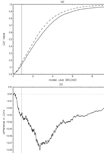
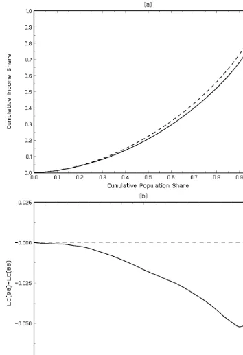
Summary statistics for the samples are provided in Table 3. There was considerable income growth over the decade from 1988 to 1998 with average real individual equivalent income increasing by 21%, and there was a corresponding decline in the poverty head-count ratio from 0.165 to 0.135. The empir-ical CDFs are plotted in Figure 1(a), and the difference in the CDFs is plotted in Figure 1(b), with a vertical line dis-tinguishing the poverty cut-off. It is apparent that the 1998 distribution tends to be to the right of the 1988 distribution, suggesting a higher level of welfare and lower poverty in the 1998 distribution, although the empirical distribution functions do cross with the 1998, distribution having greater mass than the 1988 distribution in the income range of [300, 1,700]. It is not readily apparent from CDF plots whether relative inequality is likely to be greater in the 1998 or 1988 dis-tribution. The empirical LCs are illustrated in Figure 2(a), and the differences in the LCs are shown in Figure 2(b). These fig-ures suggest that relative inequality increased over the decade with the 1988 distribution Lorenz dominating the 1998 dis-tribution. To quantify the level of inequality and poverty, and to perform inference, the 95% confidence intervals for the gener-alized Gini relative inequality and poverty indices in 1988 and 1998 are presented in Tables 4 and 5, respectively. A number of features of the interval estimates for the relative inequality indices stand out. First, the consistent asymptotic and bootstrap methods provide very similar interval estimates; the lower and upper bounds are generally equal to two decimal places. Second, all the intervals are relatively narrow in magnitude; however, the BOOT-T methods generally provided the widest interval esti-mates. Third, the grouped Gini interval estimates were sub-stantially lower than the estimates produced by the consistent procedure. Indeed, for the S-Gini relative indices, the GG(5) interval estimates are to the left of, and do not intersect with, the interval estimates produced by the consistent procedures.
The lower panels in Tables 4 and 5 contain CI estimates for the generalized Gini poverty indices. As with the inequality indices, the consistent procedures provide very similar interval estimates. As found for the relative inequality indices, the BOOT-T methods generated the widest interval estimates of the methods considered.
The next step of the analysis was to analyze the change in relative inequality and poverty between 1988 and 1998. The inference procedures were applied to the construction of CIs for the differenceI98–I88. The 95% CIs for the difference
I98–I88are presented in Table 6. The first two panels present
Table 3. Summary statistics
1988 1998
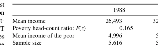
Mean income 26,493 32,231
Poverty head-count ratio:F(z) 0.165 0.135
Mean income of the poor 4,996 5,080
Sample size 5,616 5,393
the results for the S-Gini and E-Gini relative inequality indices. It is clear that all the inference procedures considered produce CIs that are to the right of the origin, and hence it can be inferred that the level of inequality significantly increased between 1988 and 1998. The values of the intervals for the difference in inequality are similar for the S-Gini indices with
d ¼{1.5, 2} but are smaller for d ¼{3, 5}. Given that the S-Gini inequality indices corresponding to higher values ofd
are more sensitive to transfers involving people toward the bottom of the income distribution, this reveals that the greatest
changes in the income distribution occurred toward the top of the income distribution, rather than at the very bottom, as illustrated in the figures.
The lower panels of Table 6 present the CI estimates for the difference in the generalized Gini poverty indices. As the interval estimates do not contain the origin, it can be concluded that the level of poverty, as measured by the normative Gini poverty indices, was not equal in the two years. However, in contrast to the change in the relative inequality indices, the CIs for the difference in the poverty indices are to the left of the
Figure 1. Comparison of U.S. Family Income Distribution based on samples from the CPS March Demographic files for 1998 and 1998. The solid vertical line corresponds to the poverty line ofz¼$8,480. (a) Family Income CDF for 1998 (——) and 1998 (- - -). (b) Difference in Family Income CDFs 1998–1988 (——) and equality ().
origin. That is, the level of poverty declined from 1988 to 1998. Interestingly, therefore, over the 1988–1998 period, the level of relative inequality significantly increased while there was a simultaneous, significant decline in poverty.
6. CONCLUSIONS
The generalized Gini indices of inequality, poverty, and welfare have many desirable normative properties. In this article, we have derived the statistical properties of consistent estimators of these indices. In contrast to a large number of
previous contributions in this area, the methods presented in this article do not require the grouping of sample observations into income quantiles, and hence the desirable normative properties of the Gini indices need not be compromised when undertaking formal hypothesis testing. The sampling variances of the Gini indices are derived by defining the indices as statis-tical functionals of LCs or GLCs, and then considering the influence function for these estimators. As a by-product of this approach, we present an alternative derivation of the variance-covariance matrix of the empirical LC and GLC estimators. The theoretical results presented in this article unify and
Figure 2. Comparison of U.S. Family Income LCs based on samples from the CPS March Demographic files for 1998 and 1998. (a) Family Income LCs for 1998 (——) and 1998 (- - - -). (b) Difference in Family Income LCs 1998–1988 (——) and equality (- - - -).
extend previous work on the sampling properties of specific members of the generalized Gini class of indices.
The consistent asymptotic inference procedures proposed in the article are compared with alternative inference procedures, based on the asymptotics for the grouped Gini estimator and various bootstrap procedures, in the context of a Monte Carlo study and an empirical application. The results of the Monte Carlo study show that the consistent asymptotic methods have
good performance in small samples, and that bootstrapping the pivotal t statistic based on the asymptotic variance esti-mator exhibited the most superior small sample performance. The methods were illustrated with a study of changes in the distribution of income in the United States over the 1990s. It was found that over the period 1988–1998 relative in-come inequality increased while poverty simultaneously declined.
Table 4. 95% CIs for generalized Gini relative inequality and poverty indices, 1988 income distribution
ASE BSE BOOT-T DB GG(10) GG(5)
S-Gini Relative Inequality Indices
d 1.5 (0.254, 0.265) (0.252, 0.266) (0.259, 0.267) (0.251, 0.268) (0.245, 0.254) (0.228, 0.237) 2 (0.389, 0.403) (0.387, 0.405) (0.387, 0.406) (0.384, 0.407) (0.383, 0.396) (0.366, 0.379) 3 (0.537, 0.553) (0.534, 0.556) (0.534, 0.556) (0.532, 0.558) (0.532, 0.548) (0.517, 0.533) 5 (0.672, 0.689) (0.669, 0.692) (0.669, 0.692) (0.667, 0.694) (0.665, 0.682) (0.645, 0.662) E-Gini Relative Inequality Indices
a 1 (0.389, 0.403) (0.387, 0.405) (0.387, 0.406) (0.384, 0.407) (0.382, 0.396) (0.366, 0.379) 2 (0.420, 0.436) (0.418, 0.438) (0.418, 0.438) (0.414, 0.440) (0.419, 0.435) (0.417, 0.432) 4 (0.453, 0.471) (0.451, 0.473) (0.451, 0.474) (0.447, 0.475) (0.453, 0.470) (0.454, 0.471) 6 (0.472, 0.490) (0.469, 0.493) (0.470, 0.493) (0.465, 0.495) (0.471, 0.490) (0.472, 0.490) S-Gini Poverty Indices
d 1 (0.063, 0.073) (0.061, 0.075) (0.061, 0.075) (0.061, 0.075) 2 (0.086, 0.098) (0.083, 0.101) (0.083, 0.101) (0.084, 0.101) 3 (0.098, 0.112) (0.095, 0.115) (0.095, 0.115) (0.096, 0.115) 5 (0.112, 0.128) (0.109, 0.130) (0.109, 0.131) (0.109, 0.131) E-Gini Poverty Indices
a 1 (0.075, 0.085) (0.072, 0.088) (0.069, 0.089) (0.073, 0.088) 2 (0.076, 0.086) (0.073, 0.089) (0.071, 0.090) (0.074, 0.089) 4 (0.077, 0.088) (0.074, 0.090) (0.072, 0.092) (0.075, 0.091) 6 (0.078, 0.088) (0.075, 0.091) (0.072, 0.092) (0.075, 0.091)
NOTE: The alternative procedures are as follows: ASE, asymptotic standard errors; BSE, bootstrap standard errors; BOOT-T, bootstrappedt-test statistic; DB, double bootstrap; GG(10), Grouped Gini based on 10 ordinates; and GG(5), grouped Gini based on 5 ordinates. Bootstrap CIs are based on 500 replications (and 100 level two replications for the double bootstrap).
Table 5. 95% CIs for generalized Gini relative inequality and poverty indices, 1998 income distribution
ASE BSE BOOT-T DB GG(10) GG(5)
S-Gini relative inequality indices
d 1.5 (0.289, 0.308) (0.288, 0.309) (0.288, 0.309) (0.288, 0.307) (0.271, 0.287) (0.248, 0.261) 2 (0.424, 0.446) (0.423, 0.448) (0.423, 0.448) (0.423, 0.446) (0.414, 0.435) (0.392, 0.411) 3 (0.565, 0.586) (0.563, 0.588) (0.563, 0.589) (0.566, 0.584) (0.561, 0.581) (0.544, 0.565) 5 (0.692, 0.711) (0.690, 0.713) (0.690, 0.713) (0.692, 0.711) (0.686, 0.705) (0.666, 0.686) E-Gini relative inequality indices
a 1 (0.424, 0.446) (0.423, 0.448) (0.423, 0.448) (0.423, 0.446) (0.414, 0.434) (0.392, 0.410) 2 (0.456, 0.480) (0.454, 0.482) (0.455, 0.482) (0.455, 0.480) (0.454, 0.477) (0.448, 0.470) 4 (0.490, 0.516) (0.488, 0.518) (0.490, 0.518) (0.490, 0.516) (0.490, 0.516) (0.490, 0.515) 6 (0.510, 0.536) (0.507, 0.538) (0.509, 0.538) (0.509, 0.536) (0.510, 0.536) (0.510, 0.536) S-Gini poverty indices
d 1 (0.050, 0.059) (0.049, 0.060) (0.049, 0.060) (0.050, 0.059) 2 (0.069, 0.081) (0.068, 0.083) (0.068, 0.083) (0.069, 0.082) 3 (0.080, 0.094) (0.079, 0.095) (0.079, 0.096) (0.080, 0.094) 5 (0.093, 0.107) (0.091, 0.109) (0.091, 0.110) (0.092, 0.108) E-Gini poverty indices
a 1 (0.060, 0.070) (0.058, 0.071) (0.057, 0.073) (0.059, 0.070) 2 (0.060, 0.071) (0.059, 0.072) (0.057, 0.074) (0.060, 0.071) 4 (0.061, 0.072) (0.060, 0.073) (0.058, 0.075) (0.061, 0.073) 6 (0.062, 0.073) (0.061, 0.074) (0.059, 0.076) (0.062, 0.073)
NOTE: Bootstrap CIs are based on 500 replications (and 100 level two replications for the double bootstrap).