Acceleration of Investment through the Stabilization Money
Sriyono Sriyono
Program Study of Magister Management Muhammadiyah University(UMSIDA)
,Sidoarjo – East Java Indonesia
ABSTRACT: Indonesia downfalls in the protracted economic crisis, one of reason is inability of the government to restore the pre- crisis level of investment in 1997, although the government has enforce Law No. 1 of 1967 Jo No 11 of 1970 on Foreign Direct Investment (FDI) and Law No. 6 Years 1968 Jo No 12 Year 1978 on Domestic Investment (DCI)., but the result is still not satisfying.
The purpose of this study is to find out whether the investment is quite effective in investmentaccelerating through the stabilization of money.This is very important because the stabilization of money will raise investments, which will finally give great impact on the condition of economy of the state.
The data of the research is collected since 1970 to 2012.The hypothesis is tested using econometric models. The main advantage of econometric modelsis it is able to handle the mutual dependence (interdependence). Besides, econometric model is an invaluable tool for understanding the way the economic system works and so to test and evaluate policy alternatives. Hypothesis is tested using multiple regression with Two Stages Least Square method.
The result of this study showed thatthrough the stabilization of money could accelerate the investment by looking at the intermediate indicators on the exchange rate but cannot be seen through the indicators of inflation.
INTRODUCTION
Many developing countries generally still have low level welfarepopulation. Economic growth is needed to catch up to the economy of the industrialized countries. The weakness of private participation ability in economic development requires the government to take a role as a driving force of national economic development.
Indonesia downfalls in a protracted economic crisis is due to the inability of the government to restore the pre-crisis level of investment in 1997 although the government has enforce Law No. 1 of 1967 Jo No. 11 of 1970 on Foreign Direct Investment (FDI) and Law No. 6 Years 1968 Jo No 12 Year 1978 on Domestic Investment (DCI). However, the results obtained have not given encouraging results.
Indonesia is currently trying to improve and recover economic growth after experiencing some kind of economic crisis. In addition, the globalization which could also pose a threat to developing countries which have relatively several flaws in the economic sector in terms of capital, human resources and technology mastery.
Various efforts to promote and enhance the investment activities as a source of sustainable economic growth in the long term have been made by the government. Increasing the value of existing investments will reduce unemployment, since the higher the unemployment rate the higher the poverty rate, this would result in lower income communities and especially will reduce national income.
There are several factors which are able to cause investments do not go as expected, those factors economic and non-economic factors. Non-economic factors can include political conditions, security factors and policy bureaucracy, while the economic factors can include the stability of the amount of circulating money. The stability of the money supply becomes an important concern in controlling the economy.
LITERATURE
Money is anything that serves as accepted medium of exchange generally. The most important concept is the narrow money, or M1, which is the number of coins and banknotes in circulation outside banks and the deposit money that can be availed. Another important monetary aggregate is broad money (M2), which consists of assets such as savings accounts plus coins, banknotes and deposits which can be turned into cheques (Samuelson, 2004:189-190). M1money is the most liquid, because the process to turn it into cash is fast and without any value loss, while M2 because it includes time deposits,has lower liquiditycompared to M1 (Nopirin I, 2007:3). Money in the narrow sense (denoted by M1) consists of currency that is outside the monetary system (outside the central bank, the government, and the creator of the banks demand deposits) and demand deposits
(demand deposits).
M1 = C + D ... 2.1
The money in the broad sense (M2) consists of M1 and quasy-money (time and savings deposits) in banks which create deposits.
M2 = M1 + TD ... 2.2
For the ease of the presentation, as well as to temporarily ignore the distinction between demand deposits and time deposits so that the equation(2.2) and (2.3) will
become:
M = C + D ... 2.3
In an economy, every time monetary base / reserve money (RM) exists, which is
determined by the size of net foreign assets held by the central bank (NRA), clean bill to
the government (NCG), bill on the banks (CB), bill to the private sector (CP), and other net assets (NOI). For ease of the presentation, it is considered that the central bank does not provide loans directly to companies and individuals, as well as the NOI is zero.
So the equation of the monetary base is the supply side (Pohan, 2008:32)
RMs = NFA +NCG + CB ... 2.4
Exceptthe NFA, the central bank can set the NCG and CB within certain limits. NFA held by central banks in general will change according to changes in the balance of payments (Pohan, 2008:33)
Where OB is overall surplus or balance of payments deficit. Base on demand, monetary base onsists of currency held by the public who wish to reserve the wanted and
owned by the creator of the banks demand deposits (R) (Pohan, 2008:33)
OB is the overall balance of payments surplus or deficit. On the demand side, the monetary base consists of currency which is owned by the public and reserved owned by
the creator of the demand deposits banks (R) (Pohan, 2008:33). RMd = C + R ... 2.6
Reserve banks consist of required reserve and excess reserve (Pohan, 2008:33)
R = RR + ER ... 2.7
By combining equation (2.2), (2.3) and (2.5),following equation will be obtained: NFA + NCG + CB = C + RR + ER ... 2.8
When CB was transferred to the right hand side of the equation and directly reduce ER, freereserve will be obtained.
NCG + NFA = C + RR + FR ... 2.9
Based on equation (2.4), equation can be obtained, namely (Pohan, 2008:33):
C = ( 𝜆 )
( 1+ 𝜆 ) M ... 2.10
In this case is the ratio of currency to deposits (𝐶)= 𝜆because some people hold 𝐷
their money in the form of deposits.
At all times banks are required to maintain reserve requirement ratio by k percent
of the savings accounts of its customers. Thus, the equation of the reserve requirement ratio is (Pohan, 2008:34):
RR = kD ... 2.11 From equation (2.11) and (2.4), following equation can be obtained:
C = 1
( 1+ 𝜆 ) M ... 2.12
By substituting equation (2.11), (2.12 and (2.13) into equation (2.10), it can be obtained:
NFA + NCG = (𝜆+𝑘)M + FR ... 2.13 ( 1+ 𝜆 )
Commercial banks provide loans with interest rate markets (r) and borrow from the central bank through the discount window at an interest rate (rd). If there is an interest
reserve and increase borrowing from the central bank. So FR (free reserves) is a function
of the difference between the interest rate r and rd. (Pohan, 2008:34) FR = f ( r – d ) ... 2.14
By substituting equation (2.15) into (2.14) then we obtain the equation: M = (1+𝜆)
( NFA + NCG ) - (1+𝜆)
f ( r - rd ) ………2.15
( 𝜆+1 ) ( 𝜆+𝑘 )
Equations 2.16 is money stock equation, which amount is influenced by the behavior of, 1, k, NFA + NCG, r and rd. Equation 2.16 shows how the central bank can control the money supply by using monetary instruments, namely open market operations, reserve and discount facility required. Open market operation executed by
purchasing government bonds by the central bank will lead to a rise in the NCG which also means an increase in the monetary base, which is then increase the supply of money.
The other way around, government bonds sale by the central bank will reduce the supply of money and RM. The increase of reserve requirement ratio (k) will reduce the multiplier
so that the supply of money decreases and the other way around a decrease in k will
increase the supply of money. Through discount policy, which is increasing, will reduce
the banks borrow from the central bank which in turn will inhibit the ability of banks to provide loans to the private sector.This will be resulted in reducing the money supply. Instead, rd decreasing would encourage banks to borrow from the central bank, which in turn will increase the money supply.
Monetary policy is not something that stands alone, but there is interdependence of the various variables in economic activities. On one hand, monetary policy is influenced by various factors in the economy, on the other hand also monetary policy directly affects the monetary and financial conditions that will in turn had an impact on the real sector condition.
Monetary policy is a policy that has been defined and implemented by Bank Indonesia to achieve and maintain rupiah stability which is done through controlling the
money supply and or interest rates. In a closed economy of a country, the country's economy do not have any interaction with other economies, the monetary policy implemented will be simpler.
Generally, there are two kinds of policies which are expansionary monetary policy also called easy money policy by increasing the money supply (money supply) and the
money (money supply). Expansionary monetary policy which is conducted by Bank Indonesia is generally taken during periods of unemployment and the national production
capacity has not been in full use. Instead, the contractive policygenerally done at states of
over-employment economy, the state in which demand exceeds the aggregate amount of
the national production capacity, the state is generally characterized by high rates of inflation.
Positively, public still has an understanding that government policy over monetary and banking sector has more power than what can effectively be achieved through the instrument.Based on this assumption it is assumed that monetary sector and banking sector has a function that can provide for the continuity of the real sector, investment, production, distribution and consumption activity.
1. The relationship between Money and Inflation
There are several reviews on the theory of inflation (Atmadjaya, 2003):
1. Quantity Theory
This theory was developedby the classical economists David Hume in Lucket
(1994), states that the amount of money in circulation was positively correlated to changes in the price level (inflation). If governments implement expansionary policies to increase the amount of money in circulation, then it willgive impact the increase in the inflation rate and vice versa. The correlation between the amount of money in circulation and the amount of the price level is proportional, meaning that if the money supply rises 3 times the price level will increase by 3 times. The monetary theory contains a weakness because some aspects do not take into consideration, those aspects are money velocity (velocity of money), the circulation of goods and services and interest rates. Yet on the other hand the
demand for money (money demand) is determined by the amount of revenue (income) and the amount of the interest rate. The assumption of the quantity theory is that
the money is used solely for the benefit of the transaction, the speed of circulation of money (velocity of money) and the economy is still in a state offull employment (Lucket,
1994:439)
of increase in the money supply and community expectations regarding price increases in the future.
2. Keynes Model
The rationale of this theory was caused by people who want to live beyond their economic capabilities, resulting in effective public demand for goods (aggregate demand) exceeds the amount of goods available (aggregate supply), this will result in the inflation gap . Limited number of inventory items is caused by the short-term production capacity
cannot be developed to offset the increase in aggregate demand.
3. Mark-up Model
The rationale of the theory of inflation is determined by two components, namely the cost of production and profit margins. Changes in the relationship between the two
components can be formulated as follows:
Price = Cost + Profit Margin… ... 2.16
Because of the large profit margin is usually specified as a percentage of total cost of production, then the formula can be translated into:
Price = Cost + (a% x Cost ) ... 2.17
Based on these similarities, it can be explained that if there is an increase in the price of the components that make up the cost of production and or increase in profit margins, it will cause an increase in the selling price of commodities in the market.
4. Structural Theory
According to this theory that inflation in developing countries is not solely a monetary phenomenon, but also a structural phenomenon or cost push inflation. This is
because the economic structure of developing countries in general are still agrarian nature, so that the economic shock which come from domestic sources, such as crop failures or things that have to do with foreign relations, e.g., worsening terms of trade, foreign debt
, and foreign exchange rates, can cause fluctuations in the price of the domestic market.
2. Currency Effect on Inflation
People hold money to buy goods and services. The more money that is needed for the transaction the more money that is held. So the quantity of money in the economy is very closely related to the amount of money exchanged in the transaction.
According to the quantity theory of inflation, the main cause of the emergence of excess demand caused by the increase in the money supply. Quantity Theory explains that the main source of inflation is due to an excess of money in circulation is multiplied (Khalwaty, 2000:15-31).
Classical theory of money demand stems from the theory about the amount of money circulating in the community. This theory is not meant to explain why a person or people are putting cash money, but rather on the role of money in the economy. In a simple classical theory of money demand equation in the form of exchange or The Equation of Exchange is the disclosure of the Quantity of Money of the ideas of American economic
thinker Irving Fisher (1867-1947) in Mankiw, 2003:78.
The relationship between the transaction and the money is shown in the following equation, called the equation of quantity (quantity equation):
M X V = P X T... 2.18
Based on equation 2.2, it can be explained that the right sideof the quantity equation tells transactions (PT). T denotes the total number of transactions during a given
period, e.g. a year. In other words, T is the number of times a year for goods and services
in exchange for money. P is the price of a particular transaction amount of money
exchanged. Products from the transaction price and the number of transactions are
PT, equal to the amount of money exchanged in a year.
The left side of the quantity equation states that the money is used for transactions
(MV). M is the quantity of money. V is the velocity of money (transactions velocity of money) and measures the rate at which money circulates in the economy. In other words,
the velocity tells us the number of times money changes hands in a given period of time (Mankiw, 2003:78-79).Besides, the above formulation is not a function but is anequation that indicates the balance between the left side and the right hand side. Based on the above formulation, it can be seen that P (inflation) is influenced by several factors, namely M (money in circulation), V (velocity of money) and T (the volume of trade). So the above
formulation can be written as:
𝑃
=
𝑀𝑉……….2.19The equation above is known as Transaction variant that shows that 3 factors that
affect the general price level is the money supply (M), velocity of circulation of money (V) and the volume of transactions (T). Formulation above also hints at the motive of
money demand for transactions as essential part of the classical monetary theory about the transaction demand for money. Money demand requires increasing if the need to
increase the money for the transaction associated with the large volume of trade. The advantage of holding money is liquid because of its ease to perform transactions (Yuliadi, 2008:42)
Because the large number of transactions is difficult to measure, the problem
T is replaced with the total output of the economy is Y, so thatthe Theory of Money
Quantity can be written as follows:
M X V = P X Y ... 2.20
Description:
M is the money supply;
V is level of velocity (the velocity) of money which is assumed constant, P is the general price index;
Y is real income
Since Y is also the total income, V is a version of the quantity equation which is
called the income velocity of money. Income velocity of money stated how many times
the money goes into a person's income in a given period.
Money demand function is an equation that shows what determines the quantity of real money balances people want to be detained.
Simple money demand equation is:
(M/P)d = kY ... 2.21
Where k is a constant that tells how much money you want to detained persons
for each income (IDR / USD). This equation states that the quantity of real money balances demanded is proportional to real income (Mankiw, 2003:80).
on the effect of money supply on inflation is also supported by previous research conducted by English (1999), and Aiyagatri et al. (1998).
3. Money and Money Exchange Rate
Monetary approach states that the foreign exchange rate as the relative price of two currenciesis determined by the balance of demand and supply of money. Monetary approach basically consists of two versions, namely the flexible price version (flexible price version) and the sticky price version (sticky price version). Sticky-price version
appeared as a result of criticism of the price flexibility in the flexible price version. According to this version, the perceived rigidity is more realistic when it comes to a short period (Ronald MacDonald: 1990).Sticky-price version of the Keynesian approach is often referred tothe supposition of the variables in the money supply is endogenous. The second assumption is not acknowledging the effectiveness of market mechanisms to resolve imbalances that occur in the short term money market.
The theory of the exchange rate with the monetary approach isa combination of the quantity theory of money with the determination of the exchange rate.
Mathematically it can be formulated as follows (Yuliadi, 2008:62):
M
V (r,Y ) Y ... 2.22 P
In which:
M is the number of nominal money P is the price level
r is the interest rate Y is real national income
The equation above indicates that the acceleration of circulation of money is a function of the interest rate and real national income which in turn will determine the rate of economic growth.So the above equation can be reformulated into (Yuliadi, 2008:62):
P=V𝑀
𝑌
………2.23
level (P *) which is converted into the magnitude of the exchange rate (E) can be formulated as follows (Yuliadi, 2008:62)
P = P*E... 2.24
Therefore, by combining those equationsabove, itcan beformulated into the following equation (Yuliadi, 2008:63):
E = ( 1 / P*) V𝑀 ...2.25 𝑌
The above equation shows that the balance exchange rate is determined by the nominal amount of money, the level of real output and the velocity of moneycirculation.
The increase in nominal money and velocity of circulation of money will decrease exchange rateproportionally, while an increasing number of real output will increase the
exchange rate.
The amount of the exchange rate (E) more completely is determined by the amount of money in relative terms, the acceleration of the circulation of money and real income between the two countries. The explanation can be formulated mathematically as follows: (Yuliadi, 2008:63)
And acceleration of money circulation is determined by the amount of real income alternative cost of holding money that can be formulated as follows (Yuliadi, 2008:63):
e m m * (y y*) (r r*) ... 2.28
By substituting the previous equation, it is obtained a formulation that describes the determination of the exchange rate according to the monetary approach, namely (Yuliadi, 2008:63):
In which the variable e, m, m *, y and y * is formulated in the form of logarithms. Determination of the balance exchange rate or the expected long-term balance exchange rate (E) is a function of the terms of trade and the long-term price level, thus formulated as follows (Yuliadi, 2008:63):
E 1() P P*
1() pM
The equation above explains that the amount of the exchange rate is determined by the amount of money proportional and proportional factors are also influenced by exogenous variables. The formulation of balance exchange rate can then be formulated as follows (Yuliadi, 2008:63):
E s() (pM / p * M*) 1
r(M / P, Y) r * E (s, M / P, Y, p, p*, M, M * ………….2.30
Increasing the amount of money in the long term in which the flexible price level will increase the price and exchange rate proportionately. Unlike the trading approach or approaches that emphasize the intensity of the elasticity of trade in goods and servicesbetween the two goods in explaining the change in the exchange rate between two currencies of the two countries.
4. Currency Effect on Exchange Rate
In the monetary approach (monetary approach), it is stated that currency
exchange rate is created from the equality or the rebalancing of stock or the total demand and supply of the currency of each country. A country's money supply is assumed to be determined by the monetary authority, but the demand for money is determined by the level of real income, the prevailing price levels and interest rates. The higher the level of income and the price level the higher demand for money by individuals and companies to finance economic transactions carried purposes will be. But if the interest rate is higher the demand for money is getting lower because the cost of storage opportunity cash is becoming more expensive. So there is an inverse relationship between the amounts of the interest rate and the demand for money (Yuliadi, 2008:64)
If the government increases the money supply, it will decrease the interest rates and stimulate abroad investment which resulting in capital outflows at the time foreign exchange rates rise (appreciation).With a rising supply of money or the money supply will raise the price of goods as measured by the terms of mone) and as well as foreign
exchange rates, as measured by the domestic currency (Herlambang, et al., 2001)
5. Impact of Inflation on Investment
Before deciding to invest, it should be realized that according to the conventional theory investment depends on the offered nominal interest rate. So the offer could be accepted if the inflation rate as expected (Bodie et al., 2003:141)
r≈ R – I ... 2.31
Fisher equation states that the nominal interest rate i is equal to the real interest
rate r i plus the expected inflation rate Ï € e:
i = ir + πe ... 2.32
ir = i –πe ... 2.33
Based on these formulations, it can be explained that the increase of inflation will increase the existing interest rate. Gillmant, Max and Michal Kejak (2009), concluded that the relationship between inflation and investment is negative, meaning that if there is an increase in inflation, there will be a decline in the value of investments and vice versa, if there is a decrease in the inflation rate, there will be an increase in the value of investments.
2.6 Relationship between Exchange Money by Investing
The results of the study conducted by Campbell et al. (2003), the influence of exchange rates on investment is negative, meaning that if there is an increase in the exchange rate of the local currency against foreign currencies, there will be a decline in the value of investments.
2.7.Simultaneous Equation Model (TSLS)
The development of the conceptual framework will provide significant input in determining the existing hypothesis, however, prior to the preparation of the conceptual framework, the framework of thinkingprocess should be made first. Thinking process in the framework of this study is the theory of the money supply, inflation theory, the exchange rate and investment theory.
which has been tested with these statistics will produce some findings, both of which relate to theoretical and empirical reality
Y1= β0 + β1 X1+ µ1
Y2= δ0 + δ1 X1+ µ2
Y3= φ0 + φ1Y1+φ3Y2+µ3
Description:
Structural equation model is as follows:
... 2.35
... 2.36
X 1 is Total of Money Supply
Y 2 Is Inflation
Y 2 is Exchange Rate
Y 3 is Investment
2.8.Hypothesis
Based on the background, the formulation of the problem, the study of theory and previous research the hypotheses are formulated as follows:
1. The money supply have a significant effect on inflation
2. The money supply significantly influence the exchange rate
3. Inflation significant effect on investment
4. The exchange rate significantly influence investment
METHODOLOGY Research Design
The approach used in this study belongs to the type of quantitative research, because the research starts from theory to analyze the influence between variables that are
observed through a deductive approach (Wan Usman, 2009:4). Besides, this study will
Research Data
The type of data used in this study is time series data for the period of 1970 to 2012. Time series data is the data that is collected, recorded, or observed at all times in a row.The data used in this study is a secondary data collected from several agencies, institutions, agencies and official institutions, such as the Central Bureau of Statistics, BankIndonesia and IFS (international financial statistics).
The available data has been collected, researched, and discussed with the competent authorities in each agency in which the data sources was obtained. Once the data is correct, then the data will be processed in accordance with the method of this study.
Data Analysis Techniques
The relationship which is analyzed in this study is the relationship between
exogenous variables (inflation and exchange rate), an intervening endogenous variable
(investment) and the dependent endogenous variable(economic growth), in which the
endogenous variables of this equation can be other exogenous variables.
Before performing regression analysis using time series of data, several tests are
needed to be done to all variablesfirst, and then to determine whether the variable is stationary or not, the stationary test is necessary.Stationary test is necessary because in
general the macroeconomic variables are nonstationary. The stationary test’s purposes is
that the mean is stable and the random error is 0, so that the regression has the obtained
ability models which are reliable and there are no spurious (Maddala, 1992:526)
It also performed the classic assumption test which includes normality test, heteroskedastic test (Priyatno, 2010:84),auto-correlation test (Kendall, 1971:8) and multicollinearity test (Winarno, 2007:5.7). In order to determine which form of analysis models is used in the conceptual model,the model is identified first. The hypotheses are tested using multiple regressions with Two Stages Least Square methods and the analytical tool used in this study is by Eviews 15.
CHAPTER 4
4.1 Analysis of Results
Classical Assumptions Test Results
1. Multicollinearity Test
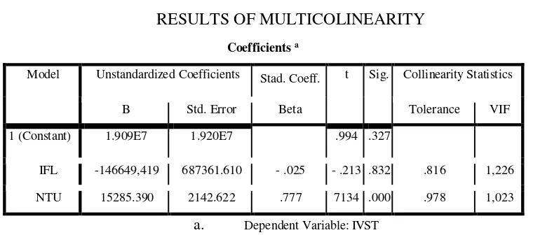
Multicollinearity test is performed on variables of inflation and exchange rate, as this variable is the independent variable that affects partially or entirely on investment, the result is as follows:
Table 4.1
RESULTS OF MULTICOLINEARITY
Coefficients a
Model Unstandardized Coefficients Stad. Coeff. t Sig. Collinearity Statistics
B Std. Error Beta Tolerance VIF
1 (Constant) 1.909E7 1.920E7 .994 .327
IFL -146649,419 687361.610 - .025 - .213 .832 .816 1,226
NTU 15285.390 2142.622 .777 7134 .000 .978 1,023
a. Dependent Variable: IVST
The existence of multicollinearity can be seen from the VIF value of each independent variable. If the VIF value between each of the independent variables is less than 5, it can be concluded that the regression model did not reveal any multicollinearity problems.
Based on the results of the tests that have been conducted,multicollinearity can be seen in Table 4.1. It appears that the coefficient of each variable is below 5. Therefore, in the models to be studied, namely inflation, interest rates and exchange rates, the multicollinearity do not occur.
2. Heterokedasitic Test
Heteroskedastic test aims to test whether the regression model of the variance of
a residual inequality is occurred fromone observation to others observation or not. The results of the heteroskedastic test using the Test Spearmensrho is presented as follows:
TABLE 4.2
Unstandardized
Residual Correlation Coefficient
1.000
Sig. (2-tailed) .
N 39
IFL Correlation Coefficient .018
Sig. (2-tailed) .912
N 39
NTU Correlation Coefficient .074
Sig. (2-tailed) .656
N 39
The Heteroskedasitic test which is done using the Test Spearmenâ € ™ s rhocan be seen in Table 4.2. In this test, it is considered the significance of the unstandardized residual value with the following procedures:
1. H 0: there is no heterokedasitic
H 1: there is heteroskedasitic
2. By using Î ± Â ± = 5%, reject H 0 P-value <Î ±
3. Because of all the variables P-Value> 0:05 then H0 is accepted
The conclusion is that the models being studied have 95% confidence level and there is one variable that has a value below the level of confidence which is the rate of interestvariable.
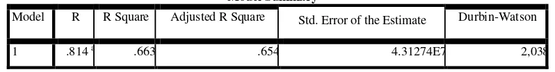
3.Autocorrelation test
Autocorrelation test aims to detect whether in a linear regression of the model correlation among errors of destruction is occurred or not.
Table 4.3
Result autocorrelation test
Model Summary b
Model R R Square Adjusted R Square Std. Error of the Estimate Durbin-Watson
1 .814 a .663 .654 4.31274E7 2,038
a.Predictors: (Constant), NTU, IFL
b.Dependent Variable: IVST
This method is based on the value of the Durbin-Watson and it is obtained that the
results of the testis presented in Table 5.3, then with Î ± = 5%, and n = 39 and k = 3, from Table Durbin-Watson it is obtained value dU = 1,658 and dL = 1.328. (See Appendix)
the values of dL and dU, it does not produce definitive conclusions (located in the area of doubt).
4. Stationary test
Before the time series of data processing is performed on stage regression, it is
necessary to have stationary test to all the variables to determine whether the variables are stationary or not. This is necessary because the time series of data in economics are
commonly not stationary, so if the test is not done then the variables used in the regression will be estimated as incorrect or spurious regression.
The test is performed by using a unit root test in order to find out whether the data
contains a unit root or not. If the variables contain a unit root, then the data is defined as
not stationary. Full result of the stationary tests that have been done on the variable inflation, exchange rate, and investment and economic growth is presented as follows:
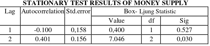
1. Stationary Test results on the variables of Inflation (IFL)
Stationary test result on the variables of inflation is presented as follows:
Table 4.4
STATIONARY TEST RESULTS OF MONEY SUPPLY Lag Autocorrelation Std.error Box- Ljung Statistic
Value df Sig
1 -0.100 0,158 0,400 1 0.527
2 0.401 0.156 7.046 2 0,030
2. Stationary Test results on the variables of Inflation (IFL)
Stationary test result on the variables of interest rateis presented as follows:
Table 4.5
STATIONARY TEST RESULTS OF INTEREST RATE Lag Autocorrelation Std. error Box-Ljung Statistic
Value df Sig
1 -0.317 0,158 4,019 1 0,045
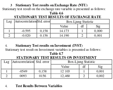
3 Stationary Test results on Exchange Rate (NTU)
Stationary test result on the exchange rate variable is presented as follows: Table 4.6
STATIONARY TEST RESULTS OF EXCHANGE RATE Lag Autocorrelation Std. error Box-Ljung Statistic
Value df Sig
1 -0.595 0,158 14.173 1 0,000
2 -0.020 0.156 14.190 2 0,001
4. Stationary Test results on Investment (IVST)
Stationary test result on Investment variables is presented as follows: Table 4.7
STATIONARY TEST RESULTS ON INVESTMENT Lag Autocorrelation Std. error Box-Ljung Statistic
Value df Sig
1 -0549 0,158 12 103 1 0,001
2 0093 0156 12,460 2 0,002
4. Test Results Between Variables
After testing the classical assumption, the proposed hypothesisis then tested. The result of the statistic test performed on all the variables is generated as follows:
4.1 Ordinary Least Square Regression Test a. Step 1
Phase 1 Results of regression relationship between the money supply and inflation, using the ordinary least squares, can be viewed as follows:
Dependent Variable: IFL Method: Least Squares Date: 08/10/13 Time: 12:10 Sample: 1970 2012
Included observations: 38 after adjusting endpoints Excluded observations: 1
Sum squared resid 6062.031 Schwarz criterion 8.101543 Log likelihood -150.2917 F-statistic 0.432658 Durbin-Watson stat 2.021673 Prob (F-statistic) 0.514872
Based on the analysis result, it can be explained that, when there is a change in the Money Supply, either increasing or additions, have meaning, these changes do not impact significantly on inflation.
The results of this study is in contrary with the Quantity Theory which explains that the main source of inflation is due to an excess of money in circulation multiplied (Khalwaty, 2000:15-31).
According to the quantity theory, the increase in the rate of money growth of 1% led to a 1% increase in the rate of inflation (Mankiw, 2003:87). The results of this study are also in contrast to the study conducted by Budina et al. (2006) and Power (2005), in those studiesit is concluded that the increase in the money supply can elevates the rate of inflation.
The phenomenon of inflation in Indonesia is not merely a short-term phenomenon and occurs occasionallyas commonly happen in other developing countries. The problem of inflation in Indonesia is a long-term inflation problemsince it occurs due to the structural constraints in the country's economy. Thus, the actiontoward the problems of inflation in Indonesia is not enough to use the short term monetary instruments, but also to make improvements in the real sector, i.e. to reduce and eliminate the factors that structurally inhibit existed in the national economy.
As we know that the onset of inflation can be derived from the demand side and the supply side. Specific task carried out by the Central Bank, in this case Bank Indonesia, is
to control inflation from the demand side, such as investment and private consumption. For example, the policy of interest rate increasing will control the public and government in spending which then reduces the aggregate demand, which in turn can reduce inflation. In addition to the increase of interest rates could also strengthen the exchange rate through an increase in the interest rate differential and Bank Indonesia may affect public
expectations through consistent and credible policies.
The cause of the other side is the supply side, this condition are beyond the control of the Central Bank. The cause of the supply-side comes from cost push inflation. These
in industrial production. This condition is usually preceded by a decrease in aggregate supply as the result of the increased cost of production. These events have occurred in
1972 and 1973 in which the oil crisis which led to the rise in oil prices. b. Step 2
Phase 1 Results of regression relationship between the money supply and the rate of money by using Ordinary Least Square analysis, can be viewed as the follows:
Dependent Variable: NTU Method: raced Squares Date: 08/10/13 Time: 12:07 Sample: 1970 2012
Included observations: 38 after adjusting endpoints
Variable Coefficient Std. Error t-Statistic Prob. JUBM1 0.059227 0.005612 10.55404 0.0000 C 1351.182 361.5180 3.737524 0.0006 R-squared 0.750653 Mean dependent var 3447.477 Adjusted R-squared 0.743914 SD dependent var 3727.693 SE of regression 1886.396 Akaike information criterion 17.97264 Sum squared resid 1.32E +08 Schwarz criterion 18.05796 Log likelihood -348.4666 F-statistic 111.3877 Durbin-Watson stat 0.573765 Prob (F-statistic) 0.000000
The money supply is chosen as an instrument of monetary control because of the amount of base money which is in control of monetary authoritarian. Assuming that the
money multiplier is stable and predictable well, the increase in the money supply will
affect the existing exchange rate movements.
Reserve circulation of foreign exchange (balance of payments) arising as a result
demand for its own currency is decreased, this will result in the appreciation of exchange rate.
2. Two Stages Least SquaresTest
b. Step 1
In the next stage, phase 2 test is conducted using TSLS method for the relationship between inflation predictors and the investment, the result can be seen as follows:
Dependent Variable: IVST Method: Least Squares Date: 08/10/13 Time: 12:27 Sample (adjusted): 1970 2012
Included observations: 38 after adjusting endpoints
Variable Coefficient Std. Error t-Statistic Prob. IFLPREDIC -42007776 5,079,227. -8.270506 0.0000 C 5.70E +08 62691114 9.088340 0.0000 R-squared 0.655177 Mean dependent var 54543926 Adjusted R-squared 0.645598 SD dependent var 72824897 SE of regression 43353869 Akaike information criterion 38.05889 Sum squared resid 6.77E +16 Schwarz criterion 38.14507 Log likelihood -721.1188 F-statistic 68.40126 Durbin-Watson stat 1.626611 Prob (F-statistic) 0.000000
Based on the results of statistical analysis, it is showed that inflation is significantly influence the investment. The result of this finding is supported by research conducted by Gillmant, Max and Michal Kejak (2009).It is concluded that the relationship between inflation and investment is negative, meaning that if there is an increase in the inflation there will be a decrease in the value of investments. This is because when inflation is high then all construction costs will be high and this will reduce the interest of investors because it costs higher than it planned.
b. Step 2
Dependent Variable: IVST Method: Least Squares Date: 08/10/13 Time: 12:37 Sample: 1970 2012
Included observations: 38 after adjusting endpoints
Variable Coefficient Std. Error t-Statistic Prob. NTUPREDIC 18023.29 2268.014 7.946725 0.0000 C -5,272,251. 10649640 -0.495064 0.6235 R-squared 0.630556 Mean dependent var 56862592 Adjusted R-squared 0.620571 SD dependent var 73304659 SE of regression 45154076 Akaike information criterion 38.13898 Sum squared resid 7.54E +16 Schwarz criterion 38.22429 Log likelihood -741.7101 F-statistic 63.15043 Durbin-Watson stat 2.032998 Prob (F-statistic) 0.000000
As an open economy, the exchange rate is one of the factors that affect the performance of the economy in general. The Effect of exchange rate on the economy are in two sides, namely the demand and supply side. On the demand side of the exchange rate depreciation will cause the price of foreign goods is relatively higher than domestic goods. This will increase the demand for domestic goods both from domestic and foreign demand towards exports.
Analysis of the demand side is enriched with the Marshall-Lener Condition
concept of price elasticity, in which the exchange rate depreciation would increase the netnumber of exports and import if price elasticity is bigger than one (Husman, 2005). From the demand side in addition that it is affected by exchange rate movements, the movement of the output is also closely related to monetary policy and fiscal policy.
Expansion of monetary policy will decrease the interest rates which further can increase investment and output .
On the other hand, from the supply side depreciation will increase the cost of imported raw materials, which in turn can lead to a decreasing in output production, so
that the net effect of the depreciation of the exchange rate of the output depends on the
c. Simultaneous relationship between Inflation and Money Exchange Rate on investment can be explained as follows:
Dependent Variable: IVST Method: Least Squares Date: 08/10/13 Time: 12:40 Sample (adjusted): 1970 2012
Included observations: 38 after adjusting endpoints
Variable Coefficient Std. Error t-Statistic Prob. NTUPREDIC 91027.08 30409.14 2.993412 0.0050 IFLPREDIC 1.38E +08 60391290 2.289136 0.0282 C -1.93E +09 8.37E +08 -2.305852 0.0272 R-squared 0.725462 Mean dependent var 54543926 Adjusted R-squared 0.709774 SD dependent var 72824897 SE of regression 39232658 Akaike information criterion 37.88357 Sum squared resid 5.39E +16 Schwarz criterion 38.01286 Log likelihood -716.7879 F-statistic 46.24352 Durbin-Watson stat 1.506197 Prob (F-statistic) 0.000000
Based on the results of the regression analysis that is performed among predictor of inflation, exchange rate predictorwith the investment, it is obtained a value of Adjusted R-squared 0.725. These findingshows that indicators of inflation and exchange rates
simultaneously affect the investment of 72.5%, while the remaining 27.5% is influenced by other factors which are not examined.
The influx of investment in a country is determined by the competitiveness of the country to another country. Competitiveness of the country was formed in addition to economic factors as well as by non-economic factors including infrastructure, political and institutional, social and cultural. The success of the state to enhance the competitiveness of the investment depends on the ability of these countries to formulate policies related to investment and business, as well as improving the quality of public service, human resource development and infrastructure in the broad sense.
Based on the model analysis, it can be concluded that stability on the money supply is very important, because if the money supply is too much it will affect the investment. This is because if the money supply is too much it will cause the fall of the exchange rate which then lead to affect the investment.
Although in this study the amount of money in circulation does not significantly affect inflation, but based on the simultaneous analysis between the rate of inflation and exchange rate, they significantly affect this investment which means that the stability of amount of money in circulation must be maintained in order to avoid over-supply, in addition,in order to make the acceleration of investment run smoothly then the factors which effects competitiveness should be minimized.
LITERATURE
Aiyagatri et al., 1998, Transaction Service, Inflation and Walfare, Journal of Political Economy. 106, 1274-1301.
Atmadjaya, Adwin S., 2003. Inflasi Di Indonesia: Sumber-sumber Penyebab dan Pengendaliannya, Jurnal Akutansi dan Keuangan, Vol 1, No.1., hal 54-67
Atmaja, Adwin Surya, 2003. Analisis Pergerakan Nilai Tukar Rupiah Terhadap Dolar Amerika Setelah Diterapkan Kebijakan Sistem Nilai Tukar Mengambang Bebas Di Indonesia, Jurnal Akutansi Dan Keuangan, Vol. 4, No. 1, Mei 2002: 69-78
Bodie, Zvi, Alex Kane, Alan J Markus, StylianosPerrakis, Peter J Ryan, 2003.
Investments, fourth Canadian edition, Mc Graw-Hill Ryerson Limited
Budina, Nina, Wojciech Maliszewski, George de Menil, Geomina Turlea , 2006, Money, Inflation and Output in Rumania, Journal of International Money and Finance, 25, 330-347.
Campbell, John Y et al., 2003. Foreign Currency For Long Term Investors, The
Economic Journal, 113 (March), C1-C25,
English. 1999, Inflation and Financual Sector Size, Journal of Monetary Economics, 44, 379-400
Herlambang, Sugiarto dan Baskara Said Kelana. 2001. Ekonomi Makro : Teori
Analisis dan Kebijakan. Jakarta : Gramedia Pustaka Utama
Kendal, G. Maurice dan William R. Buckland, A Dictionary of Statistical Terms, New York: Hafner Keynes, J.M. 1936. The General Theory of Employment,
Interest, and Money, London: Mcmillan, Inc
Khalwaty, Tajul. 2000. Inflasi dan Solusinya, Jakarta: PT. Gramedia Pustaka Umum,
Kuncoro, Mudrajad, 2007. Metode Kuantitatif, Teori Dan Aplikasi Untuk Bisnis Dan
Ekonomi, Yogyakarta: Unit Penerbit dan Percetakan (UPP) STIM YKPN
Lucket, DudleyG, 1994. Uang dan Perbankan, Jakarta: Penerbit Erlangg, Permintaan Investasi di Indonesia ( Tesis ), Magister Ilmu Ekonomi Pembangunan, Universitas Sumatra Utara (Unpublished).
Mankiw, N. Gregory, 2003. Teori Makro Ekonomi, Imam Nurmawan (alih Bahasa), Edisi V, Jakarta, Erlangga
Nopirin I, 2007, Ekonomi Moneter, Edisi 4, Buku 1,Yogyakarta: BPFE
……… II, 2007, Ekonomi Moneter, Edisi 4, Buku 2,Yogyakarta : BPFE
Nucci, Francesco and Alberto F Pozzolo, 2001., Investment and The Exchange rate: An analysis with Firm-level panel data, Europen Economic Review 45, pp 259-283
Pohan, Aulia, 2008, Kerangka kebijakan Moneter dan Implementasinya di Indonesia, Jakarta: PT. Raja Grafindo Persada.
Power, Dennis. 2005, Inside Money and The effect of Inflation, Journal of Macroeconomic, 27, 494-516
Priyatno, Duwi, 2010, Paham Analisa Statistika Data Dengan SPSS, Jakarta: PT. Buku Seru
Sarwono, Hartadi A., Perry Warjiyo, 1998. Mencari Paradigma Baru Manajemen Moneter Dalam Sistem Nilai Tukar Fleksibel, Buletin Moneter dan Perbankan, Bank Indonesia.
Sicat, Gerardo P. dan H.W. Arndt. 1991. Ilmu Ekonomi Untuk Konteks Indonesia, Nirwono ( Penerjemah ), Jakarta: LP3ES.
Siswanto, B., Kurniaty, Y., Gunawan., Binhadi, S.H., 2000. Exchange Rate Channel of Monetery Transmission in Indonesia. Dalam Perry Warjiyo dan Yuda Agung ( editor ) Transmission Mechanism of Monetery Policy In Indonesia, Directorate of Economic Research and Monetery Policy Bank Indonesia
Skousen, Mark, 2009, Sang Maestro, ”Teori-Teori Ekonomi Modern”: Sejarah
Pemikiran Sosial, Jakarta: Prenada Media Group
Smithin, John. 2003. Contraversies in Monetery Economic. Revised Edition. USA : Edward Elgar.
Undang-undang No 1 Tahun 1967 Jo No 11 Tahun 1970 tentang Penanaman Modal Asing ( PMA )
Undang-undang No 6 Tahun 1968 Jo No 12 Tahun 1978 tentang Penanaman Modal Dalam Negeri ( PMDN )
Undang-undang Nomer 13 Tahun 1968 tentang Bank Sentral
Undang-undang Nomer 23 Tahun 1999 tentang Bank Sentral
Utami, Siti Rahmi and Eno L. Inanga. Exchange Rate, Interest Rates, and Inflation raters in Indonesia : The International Fisher Effect Theory. Journal of Finance and Economic. Issue 26. Pp 151-169