108
SUPERVISED MACHINE LEARNING MODEL FOR MICRORNA EXPRESSION DATA IN CANCER
Indra Waspada1, Adi Wibowo1, and Noel Segura Meraz2
1Department of Informatics, Faculty of Science and Mathematics, Diponegoro University, Tembalang, Semarang, 50275 Indonesia
2Department of Micro-Nano Mechanichal Science and Engineering, Nagoya University, Nagoya, 464048, Japan
E-mail: [email protected], [email protected] , [email protected]
Abstract
The cancer cell gene expression data in general has a very large feature and requires analysis to find out which genes are strongly influencing the specific disease for diagnosis and drug discovery. In this paper several methods of supervised learning (decision tree, naïve bayes, neural network, and deep learning) are used to classify cancer cells based on the expression of the microRNA gene to obtain the best method that can be used for gene analysis. In this study there is no optimization and tuning of the algorithm to assess the fitness of algorithms. There are 1881 features of microRNA gene expresion, 22 cancer classes based on tissue location. A simple feature selection method is used to test the comparison of the algorithm. Expreriments were conducted with various scenarios to asses the accuracy of the classification.
Keywords: Cancer,MicroRNA, classification, Decision Tree, Naïve Bayes, Neural Network, Deep Learning
Abstrak
Data ekpresi gen sel kanker secara umum memiliki feature yang sangat banyak dan memerlukan analisa untuk mengetahui gen apa yang sangat berpengaruh terhadap spesifik penyakit untuk diagnosis dan juga penemuan obat. Pada tulisan ini beberapa metode supervised learning (decisien tree, naïve bayes, neural network, dan deep learning) digunakan untuk mengklasifikasi sel kanker berdasarkan ekpresi gen microRNA untuk mendapatkan metode terbaik yang dapat digunakan untuk analsisa gen. Dalam studi ini tidak ada optimasi dan tuning dari algoritma untuk menguji kemampuan algortima secara umum. Terdapat 1881 feature epresi gen microRNA pada 25 kelas kanker berdarkan lokasi tissue. Metode sederhana feature selection digunakan juga untuk menguji perbandingan algoritma tersebut. Exprerimen dilakukan dengan berbagai sekenario untuk menguji akurasi dari klasifikai.
Kata Kunci: Kanker,MicroRNA, Klasifikasi, Decesion Tree, Naïve Bayes, Neural Network, Deep Learning
1. Introduction
Cancer is the second deadliest disease after heart disease whith about 8.8 million cancer deaths by 2015. Moreover, one in six deaths is caused by cancer. The number of new cases are expected to increase by 70% over the next two decades [1]. It is generally recognized that cancer occurs due to gene abnormalities [2]. Gene's expression in the production rate of protein molecules are defined by genes [3]. Analyzing the gene expression profiles is the most fundamental approaches for understanding genetic abnormalities [4]. Micro Ribonucleic acid (microRNA) is known as one of the gene expressions that are very influential in
cancer cells [5]. Gene's expression data, in gene-ral, has a very large number of features and requires analysis for diagnosis and disease analy-sis or to distinguish certain types of cancer and drug discovery [6].
very large quantities features of gene expression data [9]. For gene expression data, its high dimensionality and a relative fewer quantity numbers require much more consideration and specific preprocessing to deal with. In this case, it is important to aid users by suggesting which instances to inspect, especially for large datasets.
In constructing conventional machine learning systems require technical and domain skills to convert data into appropriate internal representations to detect patterns. Conventional techniques derive from single-spaced transform-ations that are often linear and limited in their ability to process natural data in their raw form [10]. Deep learning differs from traditional machi-nes. In fact, in-depth learning allows a computa-tional model consisting of several layers of pro-cessing based on neural networks to study data representation with varying levels of abstraction [10].
In this paper, the machine learning model has been implemented in studying features of genuine gene expression data and testing it in a classification model. We apply supervised learn-ing in the form of a decision tree, naïve Bayes, and neural network compared with deep learning method in determining high-dimensional gene data pattern and achieving high accuracy. This comparison is intended to determine the reliability of the model tested in various cases, including feature selection.
The paper is structured as follows: Section 2 provides information on data and methods used for classification; Section 3 describes the results of a couple of methods from several scenarios of experiment and discussion. Finally section 4 the conclusion of paper and future works.
2. Method
Data sets
The datasets of MicroRNA expression in cancer and normal cell was occupied from National cancer institute GDC data Portal (https://portal .gdc.cancer.gov/). Table 1 shows the detail of datasets.
Decision Tree
Basically, the Decision Tree algorithm aims at obtaining a homogeneous subgroup of predefined class attributes by repeatedly repartitioning a heterogeneous sample group based on the value of the feature attribute [11], [12].
Next, divide the group into smaller and more homogeneous subgroups. Referring to the class attribute, the sample group partition is selected based on the feature attribute with the highest Information Gain value
The formula for calculating the information gain is derived from the following derivation [13]: • Information expected to classify a tuple in D
is expressed as: amount of information needed to identify the Duplication class label D. Info (D) is also known as the entropy of D.
• The amount of information required on the classification is measured using the following formula:
Tissue Cancer Normal
smaller the information, the greater the purity of the partition.
• Information Gain is defined as the difference between the original information and the new information (obtained from the partition on A), so it can be formulated as follows:
𝐺𝑎𝑖𝑛(𝐴) = 𝐼𝑛𝑓𝑜(𝐷) − 𝐼𝑛𝑓𝑜𝐴(𝐷) (3)
The iteration of the decision tree algorithm begins by partitioning the example using feature attri-butes with the largest Information Gain until it stops when the remaining value of the Information Gain attribute is below a certain threshold or the subgroup is homogeneous [11], [12]. In the end, it will produce a tree-like structure, with its branch-es being feature attributbranch-es and its leavbranch-es being subgroups. If there is an example as an input, then using the decision tree model that has been compiled it can be traced through the attribute of the input instance feature to predict the desired target attribute.
Naïve Bayes
A Naïve Bayes classifier is a simple probabilistic classifier based on applying Bayes' theorem (from Bayesian statistics) with strong (naive) indepen-dence assumptions. A more descriptive term for the underlying probability model would be in-dependent feature model. In simple terms, a Naïve Bayes classifier assumes that the presence (or absence) of a particular feature of a class (i.e. attribute) is unrelated to the presence (or absence) of any other feature. For example, a fruit may be considered to be an apple if it is red, round, and about 4 inches in diameter. Even if these features depend on each other or upon the existence of the other features, a Naïve Bayes classifier considers all of these properties to independently contribute to the probability that this fruit is an apple.
The advantage of the Naive Bayes classifier is that it only requires a small amount of training data to estimate the means and variances of the variables necessary for classification. Because independent variables are assumed, only the vari-ances of the variables for each label need to be determined and not the entire covariance matrix.
Bayes is a conditional probability model for an example problem to be classified by the vector X = (x_1 ... ..x_n) with n example.
𝑃(𝐶 𝑘|𝑥 1… 𝑥𝑛) (5)
The problem with the above formula is that if the number of n is very large, it will need a very large range of values, so the probability becomes impossible. We have a tendency to do
formula-tions on the model to provide additional use of Bayes theorem, its conditional probability is cal-culated as:
𝑝(𝐶 𝑘|𝑋) = 𝑝(𝐶 𝑘)𝑝 (𝐶 𝑘|𝑋)/𝑝(𝑋) (6)
The Bayesian probability terminology in the equation(6) can be written as Posterior =
Like-It can be rewritten as follows, by using chain rules for repeated applications on the definition of conditional probabilities as:
𝑝(𝐶 𝑘 , 𝑥1, … , 𝑥𝑛) = 𝑝(𝐶 𝑘 )𝑝(𝑥1, … , 𝑥𝑛|𝐶 𝑘) (8)
Recently the independent conditional Naive came into play: the assumption that each feature Fj is conditionally independent for every other Fi feature for j is not equal to I, given category C,
This means that based on the above indepen-dent assumption, the conditional distribution in the class C variable is:
𝑝(𝐶 𝑘|𝑥𝑖, … , 𝑥𝑗) = 1 𝑍⁄ 𝑝(𝐶 𝑘 ) ∏ 𝑝 𝑛
𝑖=1 (𝑥𝑖|𝐶 𝑘) (11)
Neural Network
Rapidminer provides neural network ope-rator. The operator uses feedforward neural net-work algorithm with backpropagation algorithm for the training. Neural networks are inspired by biological neural networks, which are then developed as mathematical models. The structure of artificial neural networks consists of connected neurons that can process and transmit information. One of the advantages of neural network is its adaptability that can change the structure of external and internal information obtained during the learning phase. The current use of neural networks is to find patterns from a set of data or to find complex models of relationships between inputs and outputs.
In the feedforward neural network, the infor-mation moves forward, one direction from the input to the output (via a hidden node) without the loop.
While backpropagation neural network (BP-NN) algorithm uses to do looping at two stages of propagation and repeated, until achieved accep-table results (good). In this algorithm the error training cycles until it reaches a small error value until it can be declared that it has reached the target.
Initially BPNN will look for an error bet-ween the original output and the desired output.
𝐸
𝑝= ∑ (𝑒
𝑖)
𝑗
𝑖=1
(12)
Where e is a nonlinear error signal. P shows pole to P; J is the number of units of output. The gradient descent method is shown in equation(13),
𝑤
𝑘,𝑖= 𝜇
𝜕𝑤
𝜕𝐸
𝑝𝑘,𝑖
(13)
Back Propagation counts errors in the output layer σj, and hidden layer. Σj using equation(14) and equation(15): duced to enhance the feed-forward with the map-ping data set input to output. The structure of the MLP Algorithm consists of multiple node layers with a directional graph that each layer is fully connected to the next layer. Each node (other than the input node) is a neuron equipped with a nonlinear activation function. Multi Layer Percep-tron utilizes back-propagation method in its train-ing phase. The arrangement of MLP consists of several layers of computing units that implement sigmoid activation functions, and are linked to each other by feed-forward.
Deep Learning
Deep Learning is based on a multi-layer feed-forward artificial neural network that is trained with stochastic gradient descent using back-propagation. The network can contain a large number of hidden layers consisting of neurons with tanh, rectifier and maxout activation func-tions. Advanced features such as adaptive learning rate, rate annealing, momentum training, dropout and L1 or L2 regularization enable high predictive accuracy. Each compute node trains a copy of the global model parameters on its local data with Settings/Preferences /General/Number of threads setting. By default, it uses the recommended num-ber of threads for the system. Only one instance of the cluster is started and it remains running until you close RapidMiner Studio.
discriminative networks with labels. Energy on the network and Probability of a unit state (Scalar T expressed as temperature) is described as equation(18)
E(s) = − ∑ aisi− ∑ sjwi
i<𝑗
i , j si (18)
A bipartite graph: No later-feed connection, feed-forward. Restricted Boltzmann Machine (R-BM) has no T factor, the rest is similar to BM. An important feature of RBM is the visible unit and hidden unit are independent, which saves on good results later: Boltzmann Machine: The state of all units: obtain-ed through the distribution of possibilities; Net-work weights: gained through training
As previously noted, RBM aims to estimate the distribution of input data. This goal is fully determined by weight and input. Energy defined for RBM is shown in equation(22):
E(v, h) = − ∑ a ivi∑ b
Distribution on the visible layer on RBM:
P(v) =1z ∑ e −E(v,h) h
(23)
Where, Z is a partition function defined as the sum of all possible configurations (v, h)
Training for RBM: Maximum Likelihood learns probability against vector x with parameter W (weight) is:
The experiment purpose is to compare the perfor-mance of several supervised machine learning methods. In determining which method is best, the performance of the method is checked by eva-luating the accuracy of the results. Classification accuracy is calculated by determining the per-centage of tuples placed in the correct class. We compute the class precision, class recall and accuracy of the method defined as
classified negative example, fn (false negative) is a incorrectly classified positive example and fp
(false positive) is a incorrectly classified negative example
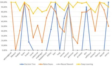
In the first scenario, all classes of cancer were tried to classify according to 1881 features of microRNA. The normal class is a combination of all normal cell samples from different types of tissue. Based on figure 1 shown that deep learning method is very stable to classify multiclass for the precision value due to the ability of deep multi layer on deep learning are able to give optimal weight of each feature for multiclass case. Similar result shown on the class recall results as can be accuracy, while the neural network is very small. Neural networks are implemented with a total of 50 iterations to reduce computational time as result the weighting of neurons is unoptimal.
to other methods with accuracy 99.12%; While other methods are as follows: naïve bayes 90.35%; Decision tree 96.49%; Neural network 91.23%.
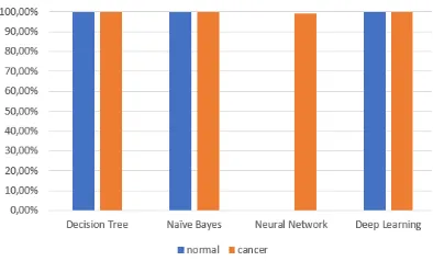
In the third scenario, a simple feature selection (expression value> 10,000) is tested on normal and cancer breast cells classification. Feature selection reduce the microRNA feature number to 3 (has-mir-10b, 21, 22). Based on figure 5 shows deep learning and neural network have the similar performance in precision, moreover other methods correspondingly have high precision value. The similar result is also perceived in the recall value as shown in figure 6. In the fourth scenario, normal and cancer of breast cells are tested for classification with selected microRNA features according to the diagnostic criteria (has-mir-10b, 125-b1,125b-2, 141, 145, 155, 191, 200a, 200b , 200c, 203a, 203b, 21,210,
30a, 92a-1, 92a-2). Bsaed on figure 7 shows that deep learning, decision tree, and neural network have a high precision results. As same as the recall according to figure 8, deep learning and neural network have high recall achievement with 100%. Moreover, the accuracy value of each method are; deep learning 100%; Naïve bayes 93.86%; Decision tree 99.12%; neural network 100%.
In the fifth scenario, normal and cancers of cervix cells are tested for classification with 1881 microRNA features. Based on figure 9 shows that nearly all methods can have high precision results, except True Negative on neural networks. The identical results shows for recall according to figure 10.
In the sixth scenario, normal and cancer of
Figure. 1. Class Precision of multi classes cancer.
Figure. 2. Class Recall of multi classes cancer.
Figure. 3. Class Precision of breast tissue between normal and cancer cell all feature
Figure. 4. Class Recall of breast tissue between normal and cancer cell all feature
Figure. 5. Class Precision of breast tissue between normal and cancer cell with feature selection on criteria >
10.000
Figure. 7. Class Precision of breast tissue between normal and cancer cell with feature selection on diagnostic criteria
(mir-21,)
Figure. 8. Class Recall of breast tissue between normal and cancer cell with feature selection on diagnostic criteria
(mir-21,)
Figure. 9. Class Precision of cervix tissue between normal and cancer cell all feature
Figure. 10. Class Recall of cervix tissue between normal and cancer cell all feature
Figure. 11. Class Precision of cervix tissue between normal and cancer cell with feature criteria > 10.000
Figure. 12. Class Recall of cervix tissue between normal and cancer cell with feature criteria > 10.000
Figure. 13. Class Precision of cervix tissue between normal and cancer cell with feature criteria diagnostic
cervical cells are tested for classification by simple feature selection (expression value > 10,000) and obtain the feature (has-mir-103a-1,103a-2,10b, 143,21,22). Based on figure 11 shows that all methods can have a perfect classification result. The equivalent results shown for recall according to figure 12.
In the last scenario, normal and cancer cervix cells are tested for classification by choosing diagnostic features with features (has-mir-146a, 155,196a-1,196a-2, 203a, 203b, 21, 221, 271, 27a, 34a). Based on figure 13 shows that only deep learning have a faultless classi-fication result. The similar results shows in figure 14 for recall.
4. Conclusion
In this paper we have presented the performance of supervised machine learning method for classification of cancer cell expression gene data. Experimental results with various scenarios, all classes, breast classes, cervical classes, and some feature selection show that deep learning method is superior to decision tree, naïve bayes and neural network methods.
Acknowledgement
This work was supported by the RISTEKDIKTI, The Republic of Indonesia. Funding Source Number: 345-21/UN7.5.1/PP/2017.
References
[1] W. M. Centre, “Cancer,” 2017. .
[2] C. Lengauer, K. W. Kinzler, and B. Vogelstein, “Genetic instabilities in human cancers.,” Nature, vol. 396, no. 6712, pp. 643–649, 1998.
[3] D. J. Lockhart and E. A. Winzeler, “Genomics, gene expression and DNA arrays.,” Nature, vol. 405, no. 6788, pp. 827–36, 2000.
[4] S. R. Poort, F. R. Rosendaal, P. H. Reitsma,
and R. M. BERTINA, “A common genetic variation in the 3'-untranslated region of the prothrombin gene is associated with elevated plasma prothrombin levels and an increase in venous thrombosis,” Blood, vol. 88, no. 10, pp. 3698–3703, 1996.
[5] H. Lan, H. Lu, X. Wang, and H. Jin, “MicroRNAs as potential biomarkers in cancer: Opportunities and challenges,”
Biomed Res. Int., vol. 2015, 2015.
[6] R. K. Singh and M. Sivabalakrishnan, “Feature selection of gene expression data for cancer classification: A review,”
Procedia Comput. Sci., vol. 50, pp. 52–57,
2015.
[7] K. Kourou, T. P. Exarchos, K. P. Exarchos, M. V. Karamouzis, and D. I. Fotiadis, “Machine learning applications in cancer prognosis and prediction,” Comput. Struct. Biotechnol. J., vol. 13, pp. 8–17, 2015.
[8] H. Chen, H. Zhao, J. Shen, R. Zhou, and Q. Zhou, “Supervised Machine Learning Model for High Dimensional Gene Data in Colon Cancer Detection,” 2015 IEEE Int. Congr. Big Data, pp. 134–141, 2015.
[9] F. Liao, H. Xu, N. Torrey, P. Road, and L. Jolla, “Multiclass cancer classification based on gene expression comparison,” vol. 2, no. 74, pp. 477–496, 2015.
[10] Y. LeCun, Y. Bengio, G. Hinton, L. Y., B. Y., and H. G., “Deep learning,” Nature, vol. 521, no. 7553, pp. 436–444, 2015.
[11] H.-M. Lee and C.-C. Hsu, “A new model for concept classification based on linear threshold unit and decision tree,” in
Proceedings of the International Joint Conference on Neural Networks (IJCNN-90-Wash D.C. IEEE/INNS), 1990, pp. 631–634.
[12] Q. J. Ross, C4.5 : programs for machine
learning. San Francisco, CA, USA: Morgan Kaufmann Publishers, 1993.