OVERVIEW
This chapter studies some of the important applications of derivatives. We
learn how derivatives are used to find extreme values of functions, to determine and
ana-lyze the shapes of graphs, to calculate limits of fractions whose numerators and
denomina-tors both approach zero or infinity, and to find numerically where a function equals zero.
We also consider the process of recovering a function from its derivative. The key to many
of these accomplishments is the Mean Value Theorem, a theorem whose corollaries
pro-vide the gateway to integral calculus in Chapter 5.
A
PPLICATIONS OF
D
ERIVATIVES
4
Extreme Values of Functions
This section shows how to locate and identify extreme values of a continuous function
from its derivative. Once we can do this, we can solve a variety of
optimization problems
in which we find the optimal (best) way to do something in a given situation.
4.1
DEFINITIONS
Absolute Maximum, Absolute Minimum
Let ƒ be a function with domain
D
. Then ƒ has an
absolute maximum
value on
D
at a point
c
if
and an
absolute minimum
value on
D
at
c
if
ƒs
x
d
Ú
ƒs
c
d
for all
x
in
D
.
ƒs
x
d
…
ƒs
c
d
for all
x
in
D
Absolute maximum and minimum values are called absolute
extrema
(plural of the Latin
extremum
). Absolute extrema are also called
global
extrema, to distinguish them from
local extrema
defined below.
For example, on the closed interval
the function
takes on
an absolute maximum value of 1 (once) and an absolute minimum value of 0 (twice). On
the same interval, the function
takes on a maximum value of 1 and a
mini-mum value of
(Figure 4.1).
Functions with the same defining rule can have different extrema, depending on the
domain.
-
1
g
s
x
d
=
sin
x
ƒs
x
d
=
cos
x
[
-
p
>
2,
p
>
2]
x y
0 1
y ⫽ sin x y ⫽ cos x
–1 2 –
2
FIGURE 4.1 Absolute extrema for the sine and cosine functions on
These values can depend on the domain of a function.
4.1 Extreme Values of Functions
245
EXAMPLE 1
Exploring Absolute Extrema
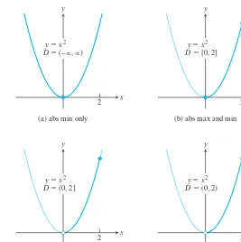
The absolute extrema of the following functions on their domains can be seen in Figure 4.2.
x 2 (a) abs min only
y ⫽ x2 D ⫽ (–⬁, ⬁)
y
x 2 (b) abs max and min
y ⫽ x2 D ⫽ [0, 2]
y
x 2 (d) no max or min
y ⫽ x2 D ⫽ (0, 2)
y
x 2 (c) abs max only
y ⫽ x2 D ⫽ (0, 2]
y
FIGURE 4.2 Graphs for Example 1.
Function rule
Domain D
Absolute extrema on D
(a)
No absolute maximum.
Absolute minimum of 0 at
(b)
[0, 2]
Absolute maximum of 4 at
Absolute minimum of 0 at
(c)
(0, 2]
Absolute maximum of 4 at
No absolute minimum.
(d)
y
=
x
2(0, 2)
No absolute extrema.
x
=
2 .
y
=
x
2x
=
0 .
x
=
2 .
y
=
x
2x
=
0 .
s
- q
,
q
d
y
=
x
2H
ISTORICALB
IOGRAPHY Daniel Bernoulli(1700–1789)
closed interval [
The following theorem asserts that a function which is continuous at every point of a
a
,
b
] has an absolute maximum and an absolute minimum value on the
The proof of The Extreme Value Theorem requires a detailed knowledge of the real
number system (see Appendix 4) and we will not give it here. Figure 4.3 illustrates
possi-ble locations for the absolute extrema of a continuous function on a closed interval [
a
,
b
].
As we observed for the function
it is possible that an absolute minimum (or
ab-solute maximum) may occur at two or more different points of the interval.
The requirements in Theorem 1 that the interval be closed and finite, and that the
function be continuous, are key ingredients. Without them, the conclusion of the theorem
need not hold. Example 1 shows that an absolute extreme value may not exist if the
inter-val fails to be both closed and finite. Figure 4.4 shows that the continuity requirement
can-not be omitted.
Local (Relative) Extreme Values
Figure 4.5 shows a graph with five points where a function has extreme values on its domain
[
a
,
b
]. The function’s absolute minimum occurs at
a
even though at
e
the function’s value is
y
=
cos
x
,
Maximum at interior point, minimum at endpoint
Minimum at interior point, maximum at endpoint
FIGURE 4.3 Some possibilities for a continuous function’s maximum and
minimum on a closed interval [a, b].
THEOREM 1
The Extreme Value Theorem
If ƒ is continuous on a closed interval [
a
,
b
], then ƒ attains both an absolute
max-imum value
M
and an absolute minimum value
m
in [
a
,
b
]. That is, there are
FIGURE 4.4 Even a single point of discontinuity can keep a function from having either a maximum or minimum value on a closed interval. The function
is continuous at every point of [0, 1]
except yet its graph over [0, 1]
does not have a highest point.
x = 1 ,
y = ex, 0… x 6 1
4.1 Extreme Values of Functions
247
smaller than at any other point
nearby
. The curve rises to the left and falls to the right
around
c
, making ƒ(
c
) a maximum locally. The function attains its absolute maximum at
d
.
x b
a c e d
Local minimum
No smaller value of f nearby.
Local minimum
No smaller value of f nearby.
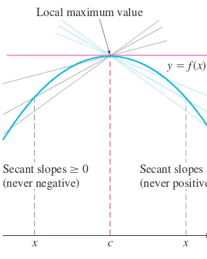
Local maximum
No greater value of f nearby.
Absolute minimum
No smaller value of f anywhere. Also a local minimum.
Absolute maximum
No greater value of f anywhere. Also a local maximum.
y ⫽ f(x)
FIGURE 4.5 How to classify maxima and minima.
DEFINITIONS
Local Maximum, Local Minimum
A function ƒ has a
local maximum
value at an interior point
c
of its domain if
A function ƒ has a
local minimum
value at an interior point
c
of its domain if
ƒs
x
d
Ú
ƒs
c
d
for all
x
in some open interval containing
c
.
ƒs
x
d
…
ƒs
c
d
for all
x
in some open interval containing
c
.
THEOREM 2
The First Derivative Theorem for Local Extreme Values
If ƒ has a local maximum or minimum value at an interior point
c
of its domain,
and if
is defined at
c
, then
ƒ
¿
s
c
d
=
0 .
ƒ
¿
We can extend the definitions of local extrema to the endpoints of intervals by defining ƒ
to have a
local maximum
or
local minimum
value
at an endpoint c
if the appropriate
in-equality holds for all
x
in some half-open interval in its domain containing
c
. In Figure 4.5,
the function ƒ has local maxima at
c
and
d
and local minima at
a
,
e
, and
b
. Local extrema
are also called
relative extrema
.
An absolute maximum is also a local maximum. Being the largest value overall, it is
also the largest value in its immediate neighborhood. Hence,
a list of all local maxima will
automatically include the absolute maximum if there is one
. Similarly,
a list of all local
minima will include the absolute minimum if there is one
.
Finding Extrema
Proof
To prove that
is zero at a local extremum, we show first that
cannot be
positive and second that
cannot be negative. The only number that is neither positive
nor negative is zero, so that is what
must be.
To begin, suppose that ƒ has a local maximum value at
(Figure 4.6) so that
for all values of
x
near enough to
c
. Since
c
is an interior point of ƒ’s
do-main,
is defined by the two-sided limit
This means that the right-hand and left-hand limits both exist at
and equal
When we examine these limits separately, we find that
(1)
Similarly,
(2)
Together, Equations (1) and (2) imply
This proves the theorem for local maximum values. To prove it for local
mini-mum values, we simply use
which reverses the inequalities in Equations (1)
and (2).
Theorem 2 says that a function’s first derivative is always zero at an interior point
where the function has a local extreme value and the derivative is defined. Hence the only
places where a function ƒ can possibly have an extreme value (local or global) are
1.
interior points where
2.
interior points where
is undefined,
3.
endpoints of the domain of ƒ.
The following definition helps us to summarize.
ƒ
¿
FIGURE 4.6 A curve with a local
maximum value. The slope at c,
simultaneously the limit of nonpositive numbers and nonnegative numbers, is zero.
DEFINITION
Critical Point
An interior point of the domain of a function ƒ where
is zero or undefined is a
critical point
of ƒ.
ƒ
¿
Thus the only domain points where a function can assume extreme values are critical
points and endpoints.
Be careful not to misinterpret Theorem 2 because its converse is false. A
differen-tiable function may have a critical point at
without having a local extreme value
there. For instance, the function
has a critical point at the origin and zero value
there, but is positive to the right of the origin and negative to the left. So it cannot have a
local extreme value at the origin. Instead, it has a
point of inflection
there. This idea is
de-fined and discussed further in Section 4.4.
Most quests for extreme values call for finding the absolute extrema of a continuous
function on a closed and finite interval. Theorem 1 assures us that such values exist;
Theo-rem 2 tells us that they are taken on only at critical points and endpoints. Often we can
4.1 Extreme Values of Functions
249
simply list these points and calculate the corresponding function values to find what the
largest and smallest values are, and where they are located.
How to Find the Absolute Extrema of a Continuous Function
ƒ
on a
Finite Closed Interval
1.
Evaluate ƒ at all critical points and endpoints.
2.
Take the largest and smallest of these values.
EXAMPLE 2
Finding Absolute Extrema
Find the absolute maximum and minimum values of
on
Solution
The function is differentiable over its entire domain, so the only critical point is
where
namely
We need to check the function’s values at
and at the endpoints
and
Critical point value:
Endpoint values:
The function has an absolute maximum value of 4 at
and an absolute minimum
value of 0 at
EXAMPLE 3
Absolute Extrema at Endpoints
Find the absolute extrema values of
on
Solution
The function is differentiable on its entire domain, so the only critical points
occur where
Solving this equation gives
a point not in the given domain. The function’s absolute extrema therefore occur at the
endpoints,
(absolute minimum), and
(absolute maximum). See
Figure 4.7.
EXAMPLE 4
Finding Absolute Extrema on a Closed Interval
Find the absolute maximum and minimum values of
on the interval
Solution
We evaluate the function at the critical points and endpoints and take the
largest and smallest of the resulting values.
The first derivative
has no zeros but is undefined at the interior point
The values of ƒ at this one
criti-cal point and at the endpoints are
Critical point value:
Endpoint values:
ƒs3d
=
s3d
2>3=
2
39 .
ƒs
-
2d
=
s
-
2d
2>3=
2
34
ƒs0d
=
0
x
=
0 .
ƒ
¿
s
x
d
=
2
3
x
-1>3
=
2
3
2
3x
[
-
2, 3] .
ƒs
x
d
=
x
2>3g
s1d
=
7
g
s
-
2d
= -
32
8
-
4
t
3=
0
or
t
=
2
32
7
1 ,
g
¿
s
t
d
=
0 .
[
-
2, 1] .
g
s
t
d
=
8
t
-
t
4x
=
0 .
x
= -
2
ƒs1d
=
1
ƒs
-
2d
=
4
ƒs0d
=
0
x
=
1 :
x
= -
2
x
=
0
x
=
0 .
ƒ
¿
s
x
d
=
2
x
=
0 ,
[
-
2, 1] .
ƒs
x
d
=
x
2(–2, –32)
(1, 7)
y ⫽ 8t ⫺ t4
– 32 7
1 –1
–2 t
y
FIGURE 4.7 The extreme values of
on (Example [-2, 1] 3).
We can see from this list that the function’s absolute maximum value is
and it
occurs at the right endpoint
The absolute minimum value is 0, and it occurs at the
interior point
(Figure 4.8).
While a function’s extrema can occur only at critical points and endpoints, not every
critical point or endpoint signals the presence of an extreme value. Figure 4.9 illustrates
this for interior points.
We complete this section with an example illustrating how the concepts we studied
are used to solve a real-world optimization problem.
EXAMPLE 5
Piping Oil from a Drilling Rig to a Refinery
A drilling rig 12 mi offshore is to be connected by pipe to a refinery onshore, 20 mi
straight down the coast from the rig. If underwater pipe costs $500,000 per mile and
land-based pipe costs $300,000 per mile, what combination of the two will give the least
expen-sive connection?
Solution
We try a few possibilities to get a feel for the problem:
(a)
Smallest amount of underwater pipe
Underwater pipe is more expensive, so we use as little as we can. We run straight to
shore (12 mi) and use land pipe for 20 mi to the refinery.
(b)
All pipe underwater (most direct route)
We go straight to the refinery underwater.
This is less expensive than plan (a).
L
11,661,900
Dollar cost
=
2544 s500,000d
20
Dollar cost
=
12s500,000d
+
20s300,000d
20 also a local maximum Local
maximum
Absolute minimum; also a local minimum y ⫽ x2/3, –2 ≤ x ≤ 3
FIGURE 4.8 The extreme values of
on occur at and
FIGURE 4.9 Critical points without
extreme values. (a) is 0 at
but has no extremum there.
4.1 Extreme Values of Functions
251
(c)
Something in between
Now we introduce the length
x
of underwater pipe and the length
y
of land-based pipe
as variables. The right angle opposite the rig is the key to expressing the relationship
be-tween
x
and
y
, for the Pythagorean theorem gives
(3)
Only the positive root has meaning in this model.
The dollar cost of the pipeline is
To express
c
as a function of a single variable, we can substitute for
x
, using Equation (3):
Our goal now is to find the minimum value of
c
(
y
) on the interval
The
first derivative of
c
(
y
) with respect to
y
according to the Chain Rule is
Setting
equal to zero gives
y
=
11
or
y
=
29 .
y
=
20
;
9
s20
-
y
d
= ;
3
4
#
12
= ;
9
16
9
A
20
-
y
B
2
=
144
25
9
A
20
-
y
B
2
=
144
+
s20
-
y
d
25
3
A
20
-
y
B
=
2
144
+
s20
-
y
d
2500,000
s20
-
y
d
=
300,000
2
144
+
s20
-
y
d
2c
¿
= -
500,000
20
-
y
2144
+
s20
-
y
d
2+
300,000 .
c
¿
s
y
d
=
500,000
#
1
2
#
2s20
-
y
ds
-
1d
2144
+
s20
-
y
d
2+
300,000
0
…
y
…
20 .
c
s
y
d
=
500,000
2
144
+
s20
-
y
d
2+
300,000
y
.
c
=
500,000
x
+
300,000
y
.
x
=
2
144
+
s20
-
y
d
2.
x
2=
12
2+
s20
-
y
d
2 12 miRig
Refinery
20 – y y
Only
lies in the interval of interest. The values of
c
at this one critical point and at
the endpoints are
The least expensive connection costs $10,800,000, and we achieve it by running the line
underwater to the point on shore 11 mi from the refinery.
252
Chapter 4: Applications of DerivativesEXERCISES 4.1
Finding Extrema from Graphs
In Exercises 1–6, determine from the graph whether the function has
any absolute extreme values on [a,b]. Then explain how your answer
is consistent with Theorem 1.
1. 2.
3. 4.
5. 6.
In Exercises 7–10, find the extreme values and where they occur.
7. 8.
In Exercises 11-14, match the table with a graph.
11. 12.
13. 14.
x ƒⴕ(x)
a does not exist
b does not exist
c ⫺1.7
x ƒⴕ(x)
a does not exist
Absolute Extrema on Finite Closed Intervals
In Exercises 15–30, find the absolute maximum and minimum values of each function on the given interval. Then graph the function. Iden-tify the points on the graph where the absolute extrema occur, and in-clude their coordinates.
In Exercises 31–34, find the function’s absolute maximum and mini-mum values and say where they are assumed.
31.
32.
33.
34.
Finding Extreme Values
In Exercises 35–44, find the extreme values of the function and where they occur.
Local Extrema and Critical Points
In Exercises 45–52, find the derivative at each critical point and deter-mine the local extreme values.
45. 46.
47. 48.
49. 50.
51.
52.
In Exercises 53 and 54, give reasons for your answers. 53. Let
a. Does exist?
b. Show that the only local extreme value of ƒ occurs at
c. Does the result in part (b) contradict the Extreme Value
Theorem?
d. Repeat parts (a) and (b) for replacing 2
bya.
54. Let
a. Does exist?
b. Does exist?
c. Does exist?
d. Determine all extrema of ƒ.
Optimization Applications
Whenever you are maximizing or minimizing a function of a single variable, we urge you to graph the function over the domain that is ap-propriate to the problem you are solving. The graph will provide in-sight before you begin to calculate and will furnish a visual context for understanding your answer.
55. Constructing a pipeline Supertankers off-load oil at a docking facility 4 mi offshore. The nearest refinery is 9 mi east of the shore point nearest the docking facility. A pipeline must be con-structed connecting the docking facility with the refinery. The pipeline costs $300,000 per mile if constructed underwater and $200,000 per mile if overland.
a. Locate Point Bto minimize the cost of the construction.
b. The cost of underwater construction is expected to increase, whereas the cost of overland construction is expected to stay constant. At what cost does it become optimal to construct the
pipeline directly to Point A?
56. Upgrading a highway A highway must be constructed to
con-nect Village Awith Village B. There is a rudimentary roadway
that can be upgraded 50 mi south of the line connecting the two villages. The cost of upgrading the existing roadway is $300,000 per mile, whereas the cost of constructing a new highway is $500,000 per mile. Find the combination of upgrading and new construction that minimizes the cost of connecting the two vil-lages. Clearly define the location of the proposed highway.
57. Locating a pumping station Two towns lie on the south side of a river. A pumping station is to be located to serve the two towns. A pipeline will be constructed from the pumping station to each of the towns along the line connecting the town and the pumping station. Locate the pumping station to minimize the amount of pipeline that must be constructed.
58. Length of a guy wire One tower is 50 ft high and another tower is 30 ft high. The towers are 150 ft apart. A guy wire is to run
from Point Ato the top of each tower.
a. Locate Point Aso that the total length of guy wire is minimal.
b. Show in general that regardless of the height of the towers, the
length of guy wire is minimized if the angles at Aare equal.
59. The function
models the volume of a box.
a. Find the extreme values of V.
b. Interpret any values found in part (a) in terms of volume of
the box.
60. The function
models the perimeter of a rectangle of dimensions xby .
a. Find any extreme values of P.
b. Give an interpretation in terms of perimeter of the rectangle
for any values found in part (a).
61. Area of a right triangle What is the largest possible area for a right triangle whose hypotenuse is 5 cm long?
62. Area of an athletic field An athletic field is to be built in the shape
of a rectanglexunits long capped by semicircular regions of radius r
at the two ends. The field is to be bounded by a 400-m racetrack.
a. Express the area of the rectangular portion of the field as a
function of xalone or ralone (your choice).
b. What values of xand rgive the rectangular portion the largest
possible area?
63. Maximum height of a vertically moving body The height of a body moving vertically is given by
withsin meters andtin seconds. Find the body’s maximum height.
64. Peak alternating current Suppose that at any given time t(in
seconds) the current i(in amperes) in an alternating current
cir-cuit is What is the peak current for this
cir-cuit (largest magnitude)?
Theory and Examples
65. A minimum with no derivative The function has
an absolute minimum value at even though ƒ is not
differ-entiable at Is this consistent with Theorem 2? Give
rea-sons for your answer.
66. Even functions If an even function ƒ(x) has a local maximum
value at can anything be said about the value of ƒ at
Give reasons for your answer.
67. Odd functions If an odd function g(x) has a local minimum
value at can anything be said about the value of g at
Give reasons for your answer.
68. We know how to find the extreme values of a continuous function
ƒ(x) by investigating its values at critical points and endpoints. But
what if there areno critical points or endpoints? What happens
then? Do such functions really exist? Give reasons for your answers. 69. Cubic functions Consider the cubic function
a. Show that ƒ can have 0, 1, or 2 critical points. Give examples
and graphs to support your argument.
b. How many local extreme values can ƒ have?
ƒsxd = ax3 + bx2 + cx + d.
70. Functions with no extreme values at endpoints
a. Graph the function
Explain why is not a local extreme value of ƒ.
b. Construct a function of your own that fails to have an extreme
value at a domain endpoint.
Graph the functions in Exercises 71–74. Then find the extreme values of the function on the interval and say where they occur.
71.
72.
73.
74.
COMPUTER EXPLORATIONS
In Exercises 75–80, you will use a CAS to help find the absolute ex-trema of the given function over the specified closed interval. Perform the following steps.
ksxd = ƒx + 1ƒ + ƒx - 3ƒ, - q 6 x 6 q hsxd = ƒx + 2ƒ - ƒx - 3ƒ, - q 6 x 6 q gsxd = ƒx - 1ƒ - ƒx - 5ƒ, -2 … x … 7 ƒsxd = ƒx - 2ƒ + ƒx + 3ƒ, -5 … x … 5
ƒs0d = 0
ƒ(x) = •sin
1
x , x 7 0
0, x = 0.
a. Plot the function over the interval to see its general behavior there.
b. Find the interior points where (In some exercises, you
may have to use the numerical equation solver to approximate a
solution.) You may want to plot as well.
c. Find the interior points where does not exist.
d. Evaluate the function at all points found in parts (b) and (c) and
at the endpoints of the interval.
e. Find the function’s absolute extreme values on the interval and
identify where they occur. 75.
76.
77.
78.
79.
80. ƒsxd = x3>4- sin x + 1
2, [0, 2p]
ƒsxd = 2x + cos x, [0, 2p]
ƒsxd = 2 + 2x - 3x2>3, [-1, 10>3]
ƒsxd = x2>3s3 - xd, [-2, 2]
ƒsxd = -x4 + 4x3 - 4x + 1, [-3>4, 3]
ƒsxd = x4 - 8x2 + 4x + 2, [-20>25, 64>25]
ƒ¿
ƒ¿
ƒ¿ =0 .
4.2 The Mean Value Theorem
255
The Mean Value Theorem
We know that constant functions have zero derivatives, but could there be a complicated
function, with many terms, the derivatives of which all cancel to give zero? What is the
re-lationship between two functions that have identical derivatives over an interval? What we
are really asking here is what functions can have a particular
kind
of derivative. These and
many other questions we study in this chapter are answered by applying the Mean Value
Theorem. To arrive at this theorem we first need Rolle’s Theorem.
Rolle’s Theorem
Drawing the graph of a function gives strong geometric evidence that between any two points
where a differentiable function crosses a horizontal line there is at least one point on the curve
where the tangent is horizontal (Figure 4.10). More precisely, we have the following theorem.
4.2
THEOREM 3
Rolle’s Theorem
Suppose that
is continuous at every point of the closed interval [
a
,
b
]
and differentiable at every point of its interior (
a
,
b
). If
then there is at least one number
c
in (
a
,
b
) at which
ƒ
¿
s
c
d
=
0 .
ƒs
a
d
=
ƒs
b
d
,
y
=
ƒs
x
d
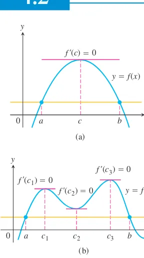
Proof
Being continuous, ƒ assumes absolute maximum and minimum values on [
a
,
b
].
These can occur only
f '(c3) ⫽ 0 f '(c2) ⫽ 0
f '(c1) ⫽ 0
f '(c) ⫽ 0
y ⫽ f(x)
y ⫽ f(x)
0 a c b
0 a c1 c2 c3 b
(a)
(b)
x x y
y
1.
at interior points where
is zero,
2.
at interior points where
does not exist,
3.
at the endpoints of the function’s domain, in this case
a
and
b
.
By hypothesis, ƒ has a derivative at every interior point. That rules out possibility (2),
leav-ing us with interior points where
and with the two endpoints
a
and
b
.
If either the maximum or the minimum occurs at a point
c
between
a
and
b
, then
by Theorem 2 in Section 4.1, and we have found a point for Rolle’s theorem.
If both the absolute maximum and the absolute minimum occur at the endpoints, then
because
it must be the case that ƒ is a constant function with
for every
Therefore
and the point
c
can be taken
anywhere in the interior (
a
,
b
).
The hypotheses of Theorem 3 are essential. If they fail at even one point, the graph
may not have a horizontal tangent (Figure 4.11).
ƒ
¿
s
x
d
=
0
x
H
[
a
,
b
] .
ƒs
x
d
=
ƒs
a
d
=
ƒs
b
d
ƒs
a
d
=
ƒs
b
d
ƒ
¿
s
c
d
=
0
ƒ
¿ =
0
ƒ
¿
ƒ
¿
a x0 b
a x0 b
a
(a) Discontinuous at an endpoint of [a, b]
(b) Discontinuous at an interior point of [a, b]
(c) Continuous on [a, b] but not differentiable at an interior point
b x x x
y y y
y ⫽ f(x) y ⫽ f(x) y ⫽ f(x)
FIGURE 4.11 There may be no horizontal tangent if the hypotheses of Rolle’s Theorem do not hold.
H
ISTORICALB
IOGRAPHYMichel Rolle (1652–1719)
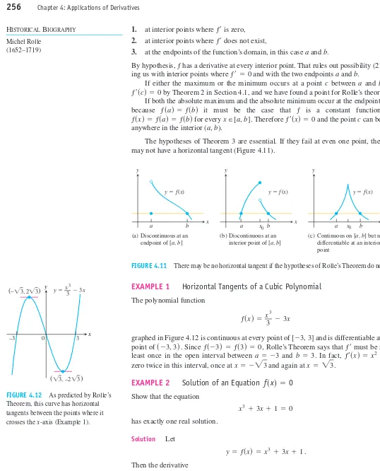
EXAMPLE 1
Horizontal Tangents of a Cubic Polynomial
The polynomial function
graphed in Figure 4.12 is continuous at every point of
and is differentiable at every
point of
Since
Rolle’s Theorem says that
must be zero at
least once in the open interval between
and
In fact,
is
zero twice in this interval, once at
and again at
EXAMPLE 2
Solution of an Equation
Show that the equation
has exactly one real solution.
Solution
Let
Then the derivative
ƒ
¿
s
x
d
=
3
x
2+
3
y
=
ƒs
x
d
=
x
3+
3
x
+
1 .
x
3+
3
x
+
1
=
0
ƒ
sxd
=
0
x
=
2
3 .
x
= -
2
3
ƒ
¿
s
x
d
=
x
2-
3
b
=
3 .
a
= -
3
ƒ
¿
ƒs
-
3d
=
ƒs3d
=
0 ,
s
-
3, 3d.
[
-
3, 3]
ƒs
x
d
=
x
33
-
3
x
x y
–3 0 3
(
–兹3, 2兹3)
(
兹3, –2兹3)
y ⫽ x3⫺ 3x 3
FIGURE 4.12 As predicted by Rolle’s Theorem, this curve has horizontal tangents between the points where it
4.2 The Mean Value Theorem
257
is never zero (because it is always positive). Now, if there were even two points
and
where ƒ(
x
) was zero, Rolle’s Theorem would guarantee the existence of a point
in between them where
was zero. Therefore, ƒ has no more than one zero. It does
in fact have one zero, because the Intermediate Value Theorem tells us that the graph of
crosses the
x
-axis somewhere between
(where
) and
(where ).
(See
Figure 4.13.)
Our main use of Rolle’s Theorem is in proving the Mean Value Theorem.
The Mean Value Theorem
The Mean Value Theorem, which was first stated by Joseph-Louis Lagrange, is a slanted
version of Rolle’s Theorem (Figure 4.14). There is a point where the tangent is parallel to
chord
AB
.
FIGURE 4.13 The only real zero of the
polynomial is the one
shown here where the curve crosses the
x-axis between -1and 0 (Example 2).
y = x3 + 3x + 1
THEOREM 4
The Mean Value Theorem
Suppose
is continuous on a closed interval [
a
,
b
] and differentiable on
the interval’s interior (
a
,
b
). Then there is at least one point
c
in (
a
,
b
) at which
(1)
ƒs
b
d
-
ƒs
a
d
b
-
a
=
ƒ
¿
s
c
d
.
y
=
ƒs
x
d
Proof
We picture the graph of ƒ as a curve in the plane and draw a line through the points
A
(
a
, ƒ(
a
)) and
B
(
b
, ƒ(
b
)) (see Figure 4.15). The line is the graph of the function
(2)
(point-slope equation). The vertical difference between the graphs of ƒ and
g
at
x
is
(3)
Figure 4.16 shows the graphs of ƒ,
g
, and
h
together.
The function
h
satisfies the hypotheses of Rolle’s Theorem on [
a
,
b
]. It is continuous
on [
a
,
b
] and differentiable on (
a
,
b
) because both ƒ and
g
are. Also,
be-cause the graphs of ƒ and
g
both pass through
A
and
B
. Therefore
at some point
This is the point we want for Equation (1).
To verify Equation (1), we differentiate both sides of Equation (3) with respect to
x
and then set
Derivative of Eq. (3) p
pwith
Rearranged
which is what we set out to prove.
ƒ
¿
s
c
d
=
ƒs
b
d
-
ƒs
a
d
Tangent parallel to chord
c b
FIGURE 4.14 Geometrically, the Mean Value Theorem says that somewhere
between Aand Bthe curve has at least
one tangent parallel to chord AB.
A(a, f(a))
FIGURE 4.15 The graph of ƒ and the
The hypotheses of the Mean Value Theorem do not require ƒ to be differentiable at
ei-ther
a
or
b
. Continuity at
a
and
b
is enough (Figure 4.17).
EXAMPLE 3
The function
(Figure 4.18) is continuous for
and
differentiable for
Since
and
the Mean Value Theorem
says that at some point
c
in the interval, the derivative
must have the value
In this (exceptional) case we can identify
c
by solving the equation
to get
A Physical Interpretation
If we think of the number
as the average change in ƒ over [
a
,
b
] and
as an instantaneous change, then the Mean Value Theorem says that at some interior
point the instantaneous change must equal the average change over the entire interval.
EXAMPLE 4
If a car accelerating from zero takes 8 sec to go 352 ft, its average
veloc-ity for the 8-sec interval is
At some point during the acceleration, the
Mean Value Theorem says, the speedometer must read exactly 30 mph
(Figure
4.19).
Mathematical Consequences
At the beginning of the section, we asked what kind of function has a zero derivative over
an interval. The first corollary of the Mean Value Theorem provides the answer.
(44 ft
>
sec)
FIGURE 4.16 The chord ABis the graph
of the function g(x). The function
gives the vertical distance
between the graphs of ƒ and gat x.
FIGURE 4.17 The function
satisfies the hypotheses (and conclusion) of the Mean Value Theorem
on even though ƒ is not
differentiable at -1and 1.
[-1, 1]
FIGURE 4.18 As we find in Example 3, is where the tangent is parallel to the chord.
FIGURE 4.19 Distance versus elapsed time for the car in Example 4.
COROLLARY 1
Functions with Zero Derivatives Are Constant
If
at each point
x
of an open interval (
a
,
b
), then
for all
where
C
is a constant.
x
H
s
a
,
b
d,
ƒs
x
d
=
C
ƒ
¿
s
x
d
=
0
4.2 The Mean Value Theorem
259
Proof
We want to show that ƒ has a constant value on the interval (
a
,
b
). We do so by
showing that if
and
are any two points in (
a
,
b
), then
Numbering
and
from left to right, we have
Then ƒ satisfies the hypotheses of the Mean
Value Theorem on
It is differentiable at every point of
and hence
continu-ous at every point as well. Therefore,
at some point
c
between and Since
throughout
(
a
,
b
), this equation translates
successively into
At the beginning of this section, we also asked about the relationship between two
functions that have identical derivatives over an interval. The next corollary tells us that
their values on the interval have a constant difference.
ƒs
x2
d
-
ƒs
x1
d
COROLLARY 2
Functions with the Same Derivative Differ by a Constant
If
at each point
x
in an open interval (
a
,
b
), then there exists a
con-Proof
At each point
the derivative of the difference function
is
Thus, on
(
a
,
b
) by Corollary 1. That is,
on (
a
,
b
), so
Corollaries 1 and 2 are also true if the open interval (
a
,
b
) fails to be finite. That is, they
re-main true if the interval is
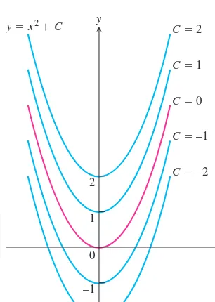
Corollary 2 plays an important role when we discuss antiderivatives in Section 4.8. It
tells us, for instance, that since the derivative of
any other
function with derivative 2
x
on
must have the formula
for some value of
C
(Figure 4.20).
EXAMPLE 5
Find the function ƒ(
x
) whose derivative is sin
x
and whose graph passes
through the point (0, 2).
Solution
Since ƒ(
x
) has the same derivative as
we know that
for some constant
C
. The value of
C
can be determined from the condition
that
(the graph of ƒ passes through (0, 2)):
The function is
Finding Velocity and Position from Acceleration
Here is how to find the velocity and displacement functions of a body falling freely from
rest with acceleration 9.8 m
>
sec
2.
ƒs
x
d
= -
cos
x
+
3 .
FIGURE 4.20 From a geometric point of view, Corollary 2 of the Mean Value Theorem says that the graphs of functions with identical derivatives on an interval can differ only by a vertical shift there. The graphs of the functions with derivative
2xare the parabolas shown
here for selected values of C.
We know that
y
(
t
) is some function whose derivative is 9.8. We also know that the
de-rivative of
is 9.8. By Corollary 2,
for some constant
C
. Since the body falls from rest,
Thus
The velocity function must be
How about the position function
s
(
t
)?
We know that
s
(
t
) is some function whose derivative is 9.8
t
. We also know that the
de-rivative of
is 9.8
t
. By Corollary 2,
for some constant
C
. If the initial height is
measured positive downward from
the rest position, then
The position function must be
The ability to find functions from their rates of change is one of the very powerful
tools of calculus. As we will see, it lies at the heart of the mathematical developments in
Chapter 5.
s
s
t
d
=
4.9
t
2+
h
.
4.9s0d
2+
C
=
h
,
and
C
=
h
.
s
s0d
=
h
,
s
s
t
d
=
4.9
t
2+
C
ƒs
t
d
=
4.9
t
2y
s
t
d
=
9.8
t
.
9.8s0d
+
C
=
0,
and
C
=
0 .
y
s0d
=
0 .
260
Chapter 4: Applications of DerivativesEXERCISES 4.2
Finding
c
in the Mean Value Theorem
Find the value or values of cthat satisfy the equation
in the conclusion of the Mean Value Theorem for the functions and in-tervals in Exercises 1–4.
1.
2.
3.
4.
Checking and Using Hypotheses
Which of the functions in Exercises 5–8 satisfy the hypotheses of the Mean Value Theorem on the given interval, and which do not? Give reasons for your answers.
5.
6.
7.
8. ƒsxd = L
sin x
x , -p … x 6 0
0, x = 0
ƒsxd = 2xs1 - xd, [0, 1]
ƒsxd = x4>5, [0, 1]
ƒsxd = x2>3, [-1, 8]
ƒsxd = 2x - 1, [1, 3]
ƒsxd = x + 1x , c1
2, 2d
ƒsxd = x2>3, [0, 1]
ƒsxd = x2 + 2x - 1, [0, 1]
ƒsbd - ƒsad
b- a = ƒ¿scd
9. The function
is zero at and and differentiable on (0, 1), but its
de-rivative on (0, 1) is never zero. How can this be? Doesn’t Rolle’s Theorem say the derivative has to be zero somewhere in (0, 1)? Give reasons for your answer.
10. For what values of a,mand bdoes the function
satisfy the hypotheses of the Mean Value Theorem on the interval [0, 2]?
Roots (Zeros)
11. a. Plot the zeros of each polynomial on a line together with the zeros of its first derivative.
i)
ii)
iii)
iv) y = x3 - 33x2 + 216x = xsx - 9dsx - 24d
y = x3 - 3x2 + 4 = sx + 1dsx - 2d2 y = x2 + 8x + 15
y = x2 - 4
ƒsxd = •
3, x = 0
-x2 + 3x + a, 0 6 x 6 1
mx + b, 1 … x … 2
x = 1
x = 0
ƒsxd = ex, 0 … x 6 1
b. Use Rolle’s Theorem to prove that between every two zeros of there lies a zero of
12. Suppose that is continuous on [a,b] and that ƒ has three zeros
in the interval. Show that has at least one zero in (a,b).
Gener-alize this result.
13. Show that if throughout an interval [a,b], then has at
most one zero in [a,b]. What if throughout [a,b] instead?
14. Show that a cubic polynomial can have at most three real zeros.
Show that the functions in Exercises 15–22 have exactly one zero in the given interval.
Finding Functions from Derivatives
23. Suppose that and that for all x. Must
for all x? Give reasons for your answer.
24. Suppose that and that for all x. Must
for all x. Give reasons for your answer.
25. Suppose that for all x. Find ƒ(2) if
a. b. c.
26. What can be said about functions whose derivatives are constant?
Give reasons for your answer.
In Exercises 27–32, find all possible functions with the given derivative.
27. a. b. c.
In Exercises 33–36, find the function with the given derivative whose
graph passes through the point P.
33.
34.
35.
36.
Finding Position from Velocity
Exercises 37–40 give the velocity and initial position of a
body moving along a coordinate line. Find the body’s position at time t.
37. 38.
39. 40.
Finding Position from Acceleration
Exercises 41–44 give the acceleration initial velocity,
and initial position of a body moving on a coordinate line. Find the
body’s position at time t.
45. Temperature change It took 14 sec for a mercury thermometer
to rise from to 100°C when it was taken from a freezer
and placed in boiling water. Show that somewhere along the way
the mercury was rising at the rate of 8.5° .
46. A trucker handed in a ticket at a toll booth showing that in 2 hours
she had covered 159 mi on a toll road with speed limit 65 mph. The trucker was cited for speeding. Why?
47. Classical accounts tell us that a 170-oar trireme (ancient Greek or
Roman warship) once covered 184 sea miles in 24 hours. Explain why at some point during this feat the trireme’s speed exceeded 7.5 knots (sea miles per hour).
48. A marathoner ran the 26.2-mi New York City Marathon in 2.2
hours. Show that at least twice the marathoner was running at ex-actly 11 mph.
49. Show that at some instant during a 2-hour automobile trip the
car’s speedometer reading will equal the average speed for the trip.
50. Free fall on the moon On our moon, the acceleration of gravity
is If a rock is dropped into a crevasse, how fast will it
be going just before it hits bottom 30 sec later?
Theory and Examples
51. The geometric mean ofaand b The geometric meanof two
positive numbers aand bis the number Show that the value
of cin the conclusion of the Mean Value Theorem for
on an interval of positive numbers
52. The arithmetic mean of aand b The arithmetic meanof two
numbers aand bis the number Show that the value of
cin the conclusion of the Mean Value Theorem for on
any interval
53. Graph the function
What does the graph do? Why does the function behave this way? Give reasons for your answers.
54. Rolle’s Theorem
a. Construct a polynomial ƒ(x) that has zeros at
b. Graph ƒ and its derivative together. How is what you see
related to Rolle’s Theorem?
c. Do and its derivative illustrate the same
phenomenon?
55. Unique solution Assume that ƒ is continuous on [a,b] and
dif-ferentiable on (a,b). Also assume that ƒ(a) and ƒ(b) have opposite
signs and that between aand b. Show that
ex-actly once between aand b.
56. Parallel tangents Assume that ƒ and g are differentiable on
[a,b] and that and Show that there is
at least one point between aand bwhere the tangents to the graphs
of ƒ and gare parallel or the same line. Illustrate with a sketch.
ƒsbd = gsbd.
the same point in the plane and the functions have the same rate of change at every point, do the graphs have to be identical? Give reasons for your answer.
58. Show that for any numbers a and b, the inequality
is true.
59. Assume that ƒ is differentiable on and that
Show that is negative at some point between aand b.
60. Let ƒ be a function defined on an interval [a,b]. What conditions
could you place on ƒ to guarantee that
where and refer to the minimum and maximum
values of on [a,b]? Give reasons for your answers.
61. Use the inequalities in Exercise 60 to estimate
for and
62. Use the inequalities in Exercise 60 to estimate
for and
63. Let ƒ be differentiable at every value of x and suppose that
that and that
a. Show that for all x.
b. Must Explain.
64. Let be a quadratic function defined on a
closed interval [a, b]. Show that there is exactly one point cin
(a, b) at which ƒ satisfies the conclusion of the Mean Value
Theorem.
262
Chapter 4: Applications of DerivativesT
T
Monotonic Functions and The First Derivative Test
In sketching the graph of a differentiable function it is useful to know where it increases
(rises from left to right) and where it decreases (falls from left to right) over an interval.
This section defines precisely what it means for a function to be increasing or decreasing
over an interval, and gives a test to determine where it increases and where it decreases.
We also show how to test the critical points of a function for the presence of local extreme
values.
Increasing Functions and Decreasing Functions
What kinds of functions have positive derivatives or negative derivatives? The answer,
pro-vided by the Mean Value Theorem’s third corollary, is this: The only functions with
posi-tive derivaposi-tives are increasing functions; the only functions with negaposi-tive derivaposi-tives are
decreasing functions.
4.3 Monotonic Functions and The First Derivative Test
263
It is important to realize that the definitions of increasing and decreasing functions
must be satisfied for
every
pair of points
and
in
I
with
Because of the
in-equality
comparing the function values, and not
some books say that ƒ is
strictly
increasing or decreasing on
I
. The interval
I
may be finite or infinite.
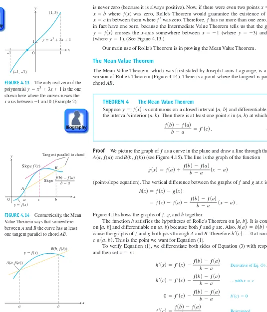
The function
decreases on
and increases on
as can be seen
from its graph (Figure 4.21). The function ƒ is monotonic on
and
but it
is not monotonic on
Notice that on the interval
the tangents have
negative slopes, so the first derivative is always negative there; for
the tangents
have positive slopes and the first derivative is positive. The following result confirms these
observations.
DEFINITIONS
Increasing, Decreasing Function
Let ƒ be a function defined on an interval
I
and let
and
be any two points in
I
.
1.
If
whenever
then ƒ is said to be
increasing
on
I
.
2.
If
whenever
then ƒ is said to be
decreasing
on
I
.
A function that is increasing or decreasing on
I
is called
monotonic
on
I
.
x
16
x
2,
COROLLARY 3
First Derivative Test for Monotonic Functions
Suppose that ƒ is continuous on [
a
,
b
] and differentiable on (
a
,
b
).
FIGURE 4.21 The function is
monotonic on the intervals and
but it is not monotonic on s- q, qd.
for some
c
between
and
The sign of the right-hand side of this equation is the same
as the sign of
because
is positive. Therefore,
if
is positive
on (
a
,
b
) and
if
is negative on (
a
,
b
).
Here is how to apply the First Derivative Test to find where a function is increasing
and decreasing. If
are two critical points for a function ƒ, and if
exists but is not
zero on the interval (
a
,
b
), then
must be positive on (
a
,
b
) or negative there (Theorem 2,
Section 3.1). One way we can determine the sign of
on the interval is simply by
evaluat-ing
for some point
x
in (
a
,
b
). Then we apply Corollary 3.
EXAMPLE 1
Using the First Derivative Test for Monotonic Functions
Find the critical points of
and identify the intervals on which ƒ is
increasing and decreasing.
Solution
The function ƒ is everywhere continuous and differentiable. The first derivative
is zero at
and
These critical points subdivide the domain of ƒ into intervals
and
on which
is either positive or negative. We determine
the sign of
by evaluating ƒ at a convenient point in each subinterval. The behavior of ƒ
is determined by then applying Corollary 3 to each subinterval. The results are
summa-rized in the following table, and the graph of ƒ is given in Figure 4.22.
Intervals
Evaluated
Sign of
Behavior of ƒ
increasing
decreasing
increasing
Corollary 3 is valid for infinite as well as finite intervals, and we used that fact in our
analysis in Example 1.
Knowing where a function increases and decreases also tells us how to test for the
na-ture of local extreme values.
First Derivative Test for Local Extrema
In Figure 4.23, at the points where ƒ has a minimum value,
immediately to the left
and
immediately to the right. (If the point is an endpoint, there is only one side to
consider.) Thus, the function is decreasing on the left of the minimum value and it is
in-creasing on its right. Similarly, at the points where ƒ has a maximum value,
imme-diately to the left and
immediately to the right. Thus, the function is increasing on
the left of the maximum value and decreasing on its right. In summary, at a local extreme
point, the sign of
ƒ
¿
s
x
d
changes.
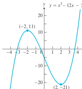
FIGURE 4.22 The function is monotonic on three separate intervals (Example 1).
x3- 12x - 5
FIGURE 4.23 A function’s first derivative tells how the graph rises and falls.
H
ISTORICALB
IOGRAPHYEdmund Halley (1656–1742)
4.3 Monotonic Functions and The First Derivative Test
265
The test for local extrema at endpoints is similar, but there is only one side to consider.
Proof
Part (1). Since the sign of
changes from negative to positive at
c,
these are
num-bers
a
and
b
such that
on (
a
,
c
) and
on (
c
,
b
). If
then
because
implies that ƒ is decreasing on [
a
,
c
]. If
then
because
implies that ƒ is increasing on [
c
,
b
]. Therefore,
for every
By definition, ƒ has a local minimum at
c
.
Parts (2) and (3) are proved similarly.
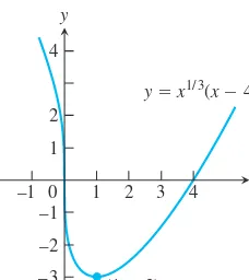
EXAMPLE 2
Using the First Derivative Test for Local Extrema
Find the critical points of
Identify the intervals on which ƒ is increasing and decreasing. Find the function’s local and
absolute extreme values.
Solution
The function ƒ is continuous at all
x
since it is the product of two continuous
functions,
and
The first derivative
is zero at
and undefined at
There are no endpoints in the domain, so the
crit-ical points
and
are the only places where ƒ might have an extreme value.
The critical points partition the
x
-axis into intervals on which
is either positive or
negative. The sign pattern of
reveals the behavior of ƒ between and at the critical points.
We can display the information in a table like the following:
Intervals
Sign of
Behavior of
ƒ
decreasing
decreasing
increasing
+
-ƒ
¿
x
7
1
0
6
x
6
1
x
6
0
ƒ
¿
ƒ
¿
x
=
1
x
=
0
x
=
0 .
x
=
1
=
4
3
x
-2>3
Q
x
-
1
R
=
4s
x
-
1d
3
x
2>3ƒ
¿
s
x
d
=
d
dx
Q
x
4>3
-
4
x
1>3R
=
4
3
x
1>3-
4
3
x
-2>3
![FIGURE 4.21The function ismonotonic on the intervals andbut it is not monotonic ons[0, - qq, dq, d.s- qƒsxd, 0] = x2](https://thumb-ap.123doks.com/thumbv2/123dok/3402711.1762577/24.684.54.210.178.342/figure-the-function-ismonotonic-intervals-andbut-monotonic-qfsxd.webp)