More
Math Into L
TEX
George Gr¨atzer
More
Math Into L
A
TEX
4th Edition
Foreword by
Rainer Sch¨opf
University of Manitoba Winnipeg, MB R3T 2N2 Canada
Cover design by Mary Burgess. Typeset by the author in LATEX.
Library of Congress Control Number:2007923503
ISBN-13: 978-0-387-32289-6 e-ISBN-13: 978-0-387-68852-7
Printed on acid-free paper.
c
2007 Springer Science+Business Media, LLC
All rights reserved. This work may not be translated or copied in whole or in part without the written permission of the publisher (Springer Science+Business Media LLC, 233 Spring Street, New York, NY 10013, USA) and the author, except for brief excerpts in connection with reviews or scholarly analysis. Use in connection with any form of information storage and retrieval, electronic adaptation, computer software, or by similar or dissimilar methodology now known or hereafter developed is forbidden.
The use in this publication of trade names, trademarks, service marks and similar terms, even if they are not identified as such, is not to be taken as an expression of opinion as to whether or not they are subject to proprietary rights.
9 8 7 6 5 4 3 2 1
without whose dedication over 15 years,
this book could not have been done
and to my four grandchildren
Danny
(11),
Anna
(8),
Emma
(2),
Short Contents
Foreword xxi
Preface to the Fourth Edition xxv
Introduction xxix
I
Short Course
1
1 Your LATEX 3
2 Typing text 7
3 Typing math 17
4 Your first article and presentation 35
II
Text and Math
59
5 Typing text 61
6 Text environments 117
7 Typing math 151
8 More math 187
III
Document Structure
245
10 LATEX documents 247
11 The AMS article document class 271
12 Legacy document classes 303
IV
Presentations and
PDFDocuments
315
13 PDFdocuments 317
14 Presentations 325
V
Customization
361
15 Customizing LATEX 363
VI
Long Documents
419
16 BIBTEX 421
17 MakeIndex 449
18 Books in LATEX 465
A Installation 489
B Math symbol tables 501
C Text symbol tables 515
D Some background 521
E LATEX and the Internet 537
F PostScript fonts 543
G LATEX localized 547
H Final thoughts 551
Bibliography 557
Contents
Foreword xxi
Preface to the Fourth Edition xxv
Acknowledgments . . . xxvii
Introduction xxix Is this book for you? . . . xxix
I
Short Course
1
1 Your LATEX 3 1.1 Your computer . . . 31.2 Sample files . . . 4
1.3 Editing cycle . . . 4
1.4 Three productivity tools . . . 5
2 Typing text 7 2.1 The keyboard . . . 8
2.2 Your first note . . . 9
2.3 Lines too wide . . . 12
2.4 More text features . . . 13
3 Typing math 17 3.1 A note with math . . . 17
3.2 Errors in math . . . 19
3.3 Building blocks of a formula . . . 22
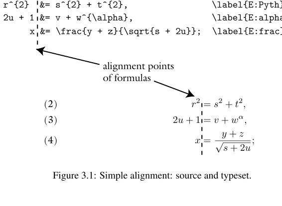
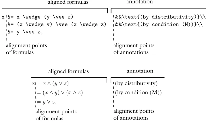
3.4 Displayed formulas . . . 27
3.4.2 Aligned formulas . . . 30
3.4.3 Cases . . . 33
4 Your first article and presentation 35 4.1 The anatomy of an article . . . 35
4.1.1 The typeset sample article . . . 41
4.2 An article template . . . 44
4.2.1 Editing the top matter . . . 44
4.2.2 Sectioning . . . 46
4.2.3 Invoking proclamations . . . 46
4.2.4 Inserting references . . . 47
4.3 On using LATEX . . . . 48
4.3.1 LATEX error messages . . . . 48
4.3.2 Logical and visual design . . . 52
4.4 Converting an article to a presentation . . . 53
4.4.1 Preliminary changes . . . 53
4.4.2 Making the pages . . . 55
4.4.3 Fine tuning . . . 55
II
Text and Math
59
5 Typing text 61 5.1 The keyboard . . . 625.1.1 Basic keys . . . 62
5.1.2 Special keys . . . 63
5.1.3 Prohibited keys . . . 63
5.2 Words, sentences, and paragraphs . . . 64
5.2.1 Spacing rules . . . 64
5.2.2 Periods . . . 66
5.3 Commanding LATEX . . . . 67
5.3.1 Commands and environments . . . 68
5.3.2 Scope . . . 71
5.3.3 Types of commands . . . 73
5.4 Symbols not on the keyboard . . . 74
5.4.1 Quotation marks . . . 75
5.4.2 Dashes . . . 75
5.4.3 Ties or nonbreakable spaces . . . 76
5.4.4 Special characters . . . 76
5.4.5 Ellipses . . . 78
5.4.6 Ligatures . . . 79
5.4.7 Accents and symbols in text . . . 79
5.4.9 Hyphenation . . . 82
5.5 Comments and footnotes . . . 85
5.5.1 Comments . . . 85
5.5.2 Footnotes . . . 87
5.6 Changing font characteristics . . . 88
5.6.1 Basic font characteristics . . . 88
5.6.2 Document font families . . . 89
5.6.3 Shape commands . . . 90
5.6.4 Italic corrections . . . 91
5.6.5 Series . . . 93
5.6.6 Size changes . . . 93
5.6.7 Orthogonality . . . 94
5.6.8 Obsolete two-letter commands . . . 94
5.6.9 Low-level commands . . . 95
5.7 Lines, paragraphs, and pages . . . 95
5.7.1 Lines . . . 96
5.7.2 Paragraphs . . . 99
5.7.3 Pages . . . 100
5.7.4 Multicolumn printing . . . 101
5.8 Spaces . . . 102
5.8.1 Horizontal spaces . . . 102
5.8.2 Vertical spaces . . . 104
5.8.3 Relative spaces . . . 105
5.8.4 Expanding spaces . . . 106
5.9 Boxes . . . 107
5.9.1 Line boxes . . . 107
5.9.2 Frame boxes . . . 109
5.9.3 Paragraph boxes . . . 110
5.9.4 Marginal comments . . . 112
5.9.5 Solid boxes . . . 113
5.9.6 Fine tuning boxes . . . 115
6 Text environments 117 6.1 Some general rules for displayed text environments . . . 118
6.2 List environments . . . 118
6.2.1 Numbered lists . . . 119
6.2.2 Bulleted lists . . . 119
6.2.3 Captioned lists . . . 120
6.2.4 A rule and combinations . . . 120
6.3 Style and size environments . . . 123
6.4 Proclamations (theorem-like structures) . . . 124
6.4.2 Proclamations with style . . . 129
6.5 Proof environments . . . 131
6.6 Tabular environments . . . 133
6.6.1 Table styles . . . 140
6.7 Tabbing environments . . . 141
6.8 Miscellaneous displayed text environments . . . 143
7 Typing math 151 7.1 Math environments . . . 152
7.2 Spacing rules . . . 154
7.3 Equations . . . 156
7.4 Basic constructs . . . 157
7.4.1 Arithmetic operations . . . 157
7.4.2 Binomial coefficients . . . 159
7.4.3 Ellipses . . . 160
7.4.4 Integrals . . . 161
7.4.5 Roots . . . 161
7.4.6 Text in math . . . 162
7.4.7 Building a formula step-by-step . . . 164
7.5 Delimiters . . . 166
7.5.1 Stretching delimiters . . . 167
7.5.2 Delimiters that do not stretch . . . 168
7.5.3 Limitations of stretching . . . 169
7.5.4 Delimiters as binary relations . . . 170
7.6 Operators . . . 170
7.6.1 Operator tables . . . 171
7.6.2 Defining operators . . . 173
7.6.3 Congruences . . . 173
7.6.4 Large operators . . . 174
7.6.5 Multiline subscripts and superscripts . . . 176
7.7 Math accents . . . 176
7.8 Stretchable horizontal lines . . . 178
7.8.1 Horizontal braces . . . 178
7.8.2 Overlines and underlines . . . 179
7.8.3 Stretchable arrow math symbols . . . 179
7.9 Formula Gallery . . . 180
8 More math 187 8.1 Spacing of symbols . . . 187
8.1.1 Classification . . . 188
8.1.2 Three exceptions . . . 188
8.1.3 Spacing commands . . . 190
8.1.5 Thephantomcommand . . . 191
8.2 Building new symbols . . . 192
8.2.1 Stacking symbols . . . 192
8.2.2 Negating and side-setting symbols . . . 194
8.2.3 Changing the type of a symbol . . . 195
8.3 Math alphabets and symbols . . . 195
8.3.1 Math alphabets . . . 196
8.3.2 Math symbol alphabets . . . 197
8.3.3 Bold math symbols . . . 197
8.3.4 Size changes . . . 199
8.3.5 Continued fractions . . . 200
8.4 Vertical spacing . . . 200
8.5 Tagging and grouping . . . 201
8.6 Miscellaneous . . . 204
8.6.1 Generalized fractions . . . 204
8.6.2 Boxed formulas . . . 205
9 Multiline math displays 207 9.1 Visual Guide . . . 207
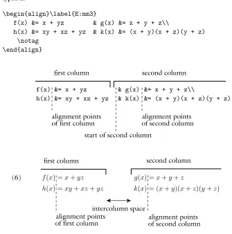
9.1.1 Columns . . . 209
9.1.2 Subsidiary math environments . . . 209
9.1.3 Adjusted columns . . . 210
9.1.4 Aligned columns . . . 210
9.1.5 Touring the Visual Guide . . . 210
9.2 Gathering formulas . . . 211
9.3 Splitting long formulas . . . 212
9.4 Some general rules . . . 215
9.4.1 General rules . . . 215
9.4.2 Subformula rules . . . 215
9.4.3 Breaking and aligning formulas . . . 217
9.4.4 Numbering groups of formulas . . . 218
9.5 Aligned columns . . . 219
9.5.1 Analignvariant . . . 221
9.5.2 eqnarray, the ancestor ofalign . . . 222
9.5.3 The subformula rule revisited . . . 223
9.5.4 Thealignatenvironment . . . 224
9.5.5 Inserting text . . . 226
9.6 Aligned subsidiary math environments . . . 227
9.6.1 Subsidiary variants . . . 227
9.6.2 Split . . . 230
9.7 Adjusted columns . . . 231
9.7.2 Arrays . . . 236
9.7.3 Cases . . . 239
9.8 Commutative diagrams . . . 240
9.9 Adjusting the display . . . 242
III
Document Structure
245
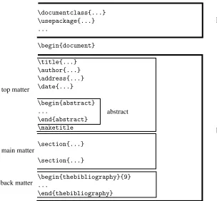
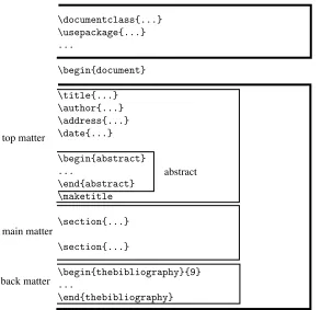
10 LATEX documents 247 10.1 The structure of a document . . . 24810.2 The preamble . . . 249
10.3 Top matter . . . 251
10.3.1 Abstract . . . 251
10.4 Main matter . . . 251
10.4.1 Sectioning . . . 252
10.4.2 Cross-referencing . . . 255
10.4.3 Floating tables and illustrations . . . 258
10.5 Back matter . . . 261
10.5.1 Bibliographies in articles . . . 261
10.5.2 Simple indexes . . . 267
10.6 Visual design . . . 268
11 The AMS article document class 271 11.1 Whyamsart? . . . 271
11.1.1 Submitting an article to the AMS . . . 271
11.1.2 Submitting an article to Algebra Universalis . . . 272
11.1.3 Submitting to other journals . . . 272
11.1.4 Submitting to conference proceedings . . . 273
11.2 The top matter . . . 273
11.2.1 Article information . . . 273
11.2.2 Author information . . . 275
11.2.3 AMS information . . . 279
11.2.4 Multiple authors . . . 281
11.2.5 Examples . . . 282
11.2.6 Abstract . . . 285
11.3 The sample article . . . 285
11.4 Article templates . . . 294
11.5 Options . . . 297
12 Legacy document classes 303
12.1 Articles and reports . . . 303
12.1.1 Top matter . . . 304
12.1.2 Options . . . 306
12.2 Letters . . . 308
12.3 The LATEX distribution . . . 310
12.3.1 Tools . . . 312
IV
Presentations and
PDFDocuments
315
13 PDFdocuments 317 13.1 PostScript andPDF . . . 31713.1.1 PostScript . . . 317
13.1.2 PDF . . . 318
13.1.3 Hyperlinks . . . 319
13.2 Hyperlinks for LATEX . . . 319
13.2.1 Usinghyperref . . . 320
13.2.2 backrefandcolorlinks . . . 320
13.2.3 Bookmarks . . . 321
13.2.4 Additional commands . . . 322
14 Presentations 325 14.1 Quick and dirtybeamer. . . 326
14.1.1 First changes . . . 326
14.1.2 Changes in the body . . . 327
14.1.3 Making things prettier . . . 328
14.1.4 Adjusting the navigation . . . 328
14.2 Babybeamers . . . 333
14.2.1 Overlays . . . 333
14.2.2 Understanding overlays . . . 335
14.2.3 More on the\onlyand\onslidecommands . . . 337
14.2.4 Lists as overlays . . . 339
14.2.5 Out of sequence overlays . . . 341
14.2.6 Blocks and overlays . . . 343
14.2.7 Links . . . 343
14.2.8 Columns . . . 347
14.2.9 Coloring . . . 348
14.3 The structure of a presentation . . . 350
14.3.1 Longer presentations . . . 354
14.3.2 Navigation symbols . . . 354
14.4 Notes . . . 355
14.6 Planning your presentation . . . 358
14.7 What did I leave out? . . . 358
V
Customization
361
15 Customizing LATEX 363 15.1 User-defined commands . . . 36415.1.1 Examples and rules . . . 364
15.1.2 Arguments . . . 370
15.1.3 Short arguments . . . 373
15.1.4 Optional arguments . . . 374
15.1.5 Redefining commands . . . 374
15.1.6 Redefining names . . . 375
15.1.7 Showing the definitions of commands . . . 376
15.1.8 Delimited commands . . . 378
15.2 User-defined environments . . . 380
15.2.1 Modifying existing environments . . . 380
15.2.2 Arguments . . . 383
15.2.3 Optional arguments with default values . . . 384
15.2.4 Short contents . . . 385
15.2.5 Brand-new environments . . . 385
15.3 A custom command file . . . 386
15.4 The sample article with user-defined commands . . . 392
15.5 Numbering and measuring . . . 398
15.5.1 Counters . . . 399
15.5.2 Length commands . . . 403
15.6 Custom lists . . . 406
15.6.1 Length commands for thelistenvironment . . . 407
15.6.2 Thelistenvironment . . . 409
15.6.3 Two complete examples . . . 411
15.6.4 Thetrivlistenvironment . . . 414
15.7 The dangers of customization . . . 415
VI
Long Documents
419
16 BIBTEX 421 16.1 The database . . . 42316.1.1 Entry types . . . 423
16.1.2 Typing fields . . . 426
16.1.3 Articles . . . 428
16.1.5 Conference proceedings and collections . . . 430
16.1.6 Theses . . . 433
16.1.7 Technical reports . . . 434
16.1.8 Manuscripts and other entry types . . . 435
16.1.9 Abbreviations . . . 436
16.2 Using BIBTEX . . . 437
16.2.1 Sample files . . . 437
16.2.2 Setup . . . 439
16.2.3 Four steps of BIBTEXing . . . 440
16.2.4 BIBTEX rules and messages . . . 443
16.2.5 Submitting an article . . . 446
16.3 Concluding comments . . . 446
17 MakeIndex 449 17.1 Preparing the document . . . 449
17.2 Index commands . . . 453
17.3 Processing the index entries . . . 459
17.4 Rules . . . 462
17.5 Multiple indexes . . . 463
17.6 Glossary . . . 464
17.7 Concluding comments . . . 464
18 Books in LATEX 465 18.1 Book document classes . . . 466
18.1.1 Sectioning . . . 466
18.1.2 Division of the body . . . 467
18.1.3 Document class options . . . 468
18.1.4 Title pages . . . 469
18.1.5 Springer’s document class for monographs . . . 469
18.2 Tables of contents, lists of tables and figures . . . 473
18.2.1 Tables of contents . . . 473
18.2.2 Lists of tables and figures . . . 475
18.2.3 Exercises . . . 476
18.3 Organizing the files for a book . . . 476
18.3.1 The folders and the master document . . . 477
18.3.2 Inclusion and selective inclusion . . . 478
18.3.3 Organizing your files . . . 479
18.4 Logical design . . . 479
18.5 Final preparations for the publisher . . . 482
A Installation 489
A.1 LATEX on a PC . . . 490
A.1.1 InstallingMiKTeX. . . 490
A.1.2 InstallingWinEdt. . . 490
A.1.3 The editing cycle . . . 491
A.1.4 Making a mistake . . . 491
A.1.5 Three productivity tools . . . 494
A.1.6 An important folder . . . 494
A.2 LATEX on a Mac . . . 495
A.2.1 Installations . . . 495
A.2.2 Working withTeXShop. . . 496
A.2.3 The editing cycle . . . 498
A.2.4 Making a mistake . . . 498
A.2.5 Three productivity tools . . . 498
A.2.6 An important folder . . . 499
B Math symbol tables 501 B.1 Hebrew and Greek letters . . . 501
B.2 Binary relations . . . 503
B.3 Binary operations . . . 506
B.4 Arrows . . . 507
B.5 Miscellaneous symbols . . . 508
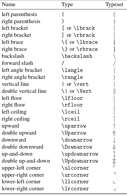
B.6 Delimiters . . . 509
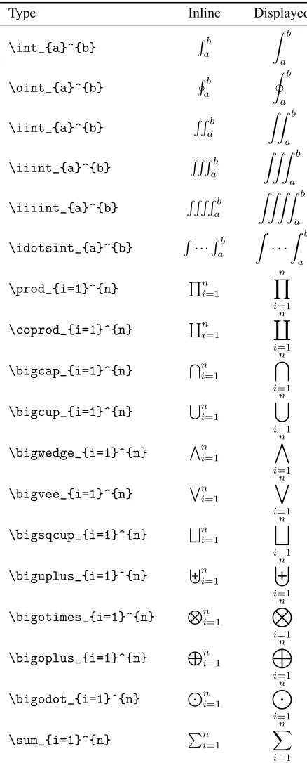
B.7 Operators . . . 510
B.7.1 Large operators . . . 511
B.8 Math accents and fonts . . . 512
B.9 Math spacing commands . . . 513
C Text symbol tables 515 C.1 Some European characters . . . 515
C.2 Text accents . . . 516
C.3 Text font commands . . . 516
C.3.1 Text font family commands . . . 516
C.3.2 Text font size changes . . . 517
C.4 Additional text symbols . . . 518
C.5 Additional text symbols with T1 encoding . . . 519
C.6 Text spacing commands . . . 520
D Some background 521 D.1 A short history . . . 521
D.1.1 TEX . . . 521
D.1.2 LATEX 2.09 andAMS-TEX . . . 522
D.1.4 More recent developments . . . 524
D.2 Structure . . . 525
D.2.1 Using LATEX . . . 525
D.2.2 AMS packages revisited . . . 528
D.3 How LATEX works . . . 528
D.3.1 The layers . . . 528
D.3.2 Typesetting . . . 529
D.3.3 Viewing and printing . . . 530
D.3.4 LATEX’s files . . . 531
D.4 Interactive LATEX . . . 534
D.5 Separating form and content . . . 535
E LATEX and the Internet 537 E.1 Obtaining files from the Internet . . . 537
E.2 The TEX Users Group . . . 541
E.3 Some useful sources of LATEX information . . . 542
F PostScript fonts 543 F.1 The Times font and MathTıme . . . 544
F.2 Lucida Bright fonts . . . 546
F.3 More PostScript fonts . . . 546
G LATEX localized 547 H Final thoughts 551 H.1 What was left out? . . . 551
H.1.1 LATEX omissions . . . 551
H.1.2 TEX omissions . . . 552
H.2 Further reading . . . 553
H.3 What’s coming . . . 554
Bibliography 557
Foreword
It was the autumn of 1989—a few weeks before the Berlin wall came down, President George H. W. Bush was president, and the American Mathematical Society decided to outsource TEX programming to Frank Mittelbach and me.
Why did the AMS outsource TEX programming to us? This was, after all, a decade before the words “outsourcing” and “off-shore” entered the lexicon. There were many American TEX experts. Why turn elsewhere?
For a number of years, the AMS tried to port the mathematical typesetting features ofAMS-TEX to LATEX, but they made little progress with the AMSFonts. Frank and I
had just published the New Font Selection Scheme for LATEX, which went a long way
to satisfy what they wanted to accomplish. So it was logical that the AMS turned to us to add AMSFonts to LATEX. Being young and enthusiastic, we convinced the AMS
that theAMS-TEX commands should be changed to conform to the LATEX standards.
Michael Downes was assigned as our AMS contact; his insight was a tremendous help. We already had LATEX-NFSS, which could be run in two modes: compatible with
the old LATEX or enabled with the new font features. We added the reworkedAMS
-TEX code to LATEX-NFSS, thus giving birth toAMS-LATEX, released by the AMS at the
August 1990 meeting of the International Mathematical Union in Kyoto.
AMS-LATEX was another variant of LATEX. Many installations had several LATEX
variants to satisfy the needs of their users: with old and new font changing commands, with and without AMS-LATEX, a single and a multi-language version. We decided
to develop a Standard LATEX that would reconcile all the variants. Out of a group of
interested people grew what was later called theLATEX3 team—and the LATEX3 project
got underway. The team’s first major accomplishment was the release of LATEX 2ε in
June 1994. This standard LATEX incorporates all the improvements we wanted back in
1989. It is now very stable and it is uniformly used.
Under the direction of Michael Downes, ourAMS-LATEX code was turned into
team recognizes that these are special; we call them “required packages” because they are part and parcel of a mathematician’s standard toolbox.
Since then a lot has been achieved to make an author’s task easier. A tremendous number of additional packages are available today. TheLATEX Companion,2nd edition, describes many of my favorite packages.
George Gr¨atzer got involved with these developments in 1990, when he got his copy ofAMS-LATEX in Kyoto. The documentation he received explained thatAMS
-LATEX is a LATEX variant—read Lamport’s LATEX book to get the proper background.
AMS-LATEX is notAMS-TEX either—read Spivak’sAMS-TEX book to get the proper
background. The rest of the document explained in what wayAMS-LATEX differs from
LATEX andAMS-TEX. Talk about a steep learning curve . . .
Luckily, George’s frustration working through this nightmare was eased by a lengthy e-mail correspondence with Frank and lots of telephone calls to Michael. Three years of labor turned into his first book on LATEX, providing a “simple introduction to
AMS-LATEX”.
This fourth edition is more mature, but preserves what made his first book such a success. Just as in the first book, Part I is a short introduction for the beginner, dramatically reducing the steep learning curve of a few weeks to a few hours. The rest of the book is a detailed presentation of what you may need to know. George “teaches by example”. You find in this book many illustrations of even the simplest concepts. For articles, he presents the LATEX source file and the typeset result
side-by-side. For formulas, he discusses the building blocks with examples, presents aFormula Gallery,and aVisual Guideto multiline formulas.
Going forth and creating “masterpieces of the typesetting art”—as Donald Knuth put it at the end of theTEXbook—requires a fair bit of initiation. This is the book for the LATEX beginner as well as for the advanced user. You just start at a different point.
The topics covered include everything you need for mathematical publishing.
Starting from scratch, by installing and running LATEX on your own computer
Instructions on creating articles, from the simple to the complex
Converting an article to a presentation
Customize LATEX to your own needs
The secrets of writing a book
Where to turn to get more information or to download updates
The many examples are complemented by a number of easily recognizable fea-tures:
Rules which you must follow
Tips on how to achieve some specific results
Experiments to show what happens when you make mistakes—sometimes, it can be
difficult to understand what went wrong when all you see is an obscure LATEX
This book teaches you how to convert your mathematical masterpieces into typo-graphical ones, giving you a lot of useful advice on the way. How to avoid the traps for the unwary and how to make your editor happy. And hopefully, you’ll experience the fascination of doing it right. Using good typography to better express your ideas.
If you want to learn LATEX, buy this book and start with theShort Course. If you
can have only one book on LATEX next to your computer, this is the one to have. And if
you want to learn about the world of LATEX packages, also buy a second book, theLATEX Companion,2nd edition.
Preface to the
Fourth Edition
This is my fourth full-sized book on LATEX.
The first book,Math into TEX: A Simple Introduction toAMS-LATEX [19], written in 1991 and 1992, introduced the brand newAMS-LATEX, a LATEX variant not
compati-ble with the LATEX of the time, LATEX 2.09. It brought together the features of LATEX and
the math typesetting abilities ofAMS-TEX, the AMS typesetting language.
The second book, Math into LATEX: An Introduction to LATEX and AMS-LATEX [27], written in 1995, describes the new LATEX introduced by the LATEX3 team and the
AMS typesetting features implemented as extensions of LATEX, called packages.
The third book,Math into LATEX, 3rd edition [30], published in 2000, reports on the same system. By 2000, both the “new” LATEX and the AMS packages were quite
mature. The feverish debugging of the new LATEX every six months bore fruit. LATEX
became very stable. It has changed little since 2000. Version 2.0 of the AMS packages was released and it also became very stable. The third book reports on a rock solid typesetting system.
What also changed between 1995 and 2000 is the widespread use of the Internet. Several chapters of the third book deal with the impact of the Internet on mathematical publications.
Now, seven years later, we can still report that LATEX—no longer new—and the
AMS packages have changed very little. However, the impact of the Internet became even more important. Computers also changed. They are now much more powerful. When I started typesetting math with LATEX, it took two and a half minutes to typeset
Circumincession
So this is the first big change compared to the previous books. In this book, we roll TEX, LATEX, and the AMS packages into one, and we call it simply LATEX. This results
in a great simplification in the exposition and makes the learning curve a little less steep.
I am sure with some advanced users this will prove to be a controversial decision. They want to know where a command is defined. For the beginner and the non-expert user this does not make any difference. What matters is that the command they need be available when they need it.
From the beginner’s point of view, this approach is very beneficial. Take as an example the\textcommand. In all three of my books, we first introduce the LATEX
command \mboxfor typing text in math formulas. After half a page of discussion comes the sentence: “It is better to enter text in formulas with the\text command provided by theamsmathpackage.” Then another half page discusses the command \text. In this book, we ignore\mboxand go right-away to\text. You do not have to do anything to access the command, theamsmathpackage is always loaded for you. And what to do if you want to find out where a command is defined. Now for both the PC and the Mac, you can easily search for contents of files. Do you want to know where a command is defined? Search for it and it is easy to find the file in which it is introduced.
Presentations
The second big change is the widespread acceptance of the AdobePDFformat. As a result, the majority of the lectures today at math meetings are given aspresentations, PDF files projected to screens using computers. Blackboards and whiteboards have largely disappeared and computer projections are overtaking projectors. So this book takes up presentations as a major topic, introducing it in Part I and discussing it in detail in Chapter 14.
Installations
In the third book, I report a recurring question that comes up from my readers again and again:
Can you help me get started from scratch, covering everything from installing a work-ing LATEX system to the rudiments of text editing?
And here is the third big change that has happened in the last few years. While ear-lier there were dozens of different LATEX implementations and hundreds of text editors,
install LATEX, it is easy for me to help you. Appendix A provides instructions on how
to install these systems.
Acknowledgments
This book is based, of course, on the three previous books. I would like to thank the many people who read and reread those earlier manuscripts.
The editors Richard Ribstein, Thomas R. Scavo, Claire M. Connelly.
The professionals Michael Downes (the project leader for the AMS), Frank
Mittel-bach and David Carlisle (of the LATEX3 team) read and criticized some or all of
the three books.
Oren Patashnik (the author of BIBTEX) carefully corrected the BIBTEX chapter for two editions.
Sebastian Rahtz (the author of thehyperrefpackage and coauthor ofThe LATEX Web Companion[18]) read the chapter on the Web in the third book.
Last but not least, Barbara Beeton of the AMS read all three books with incredi-ble insight.
The volunteers for the second book alone, there were 29—listed there. The
volun-teer readers made tremendous contributions and offered hundreds of pages of corrections. No expert can substitute for the diverse points of view I got from them.
My colleagues especially Michael Doob, Harry Lakser, and Craig Platt, who have
been very generous with their time.
The publishers Edwin Beschler, who believed in the project from the very beginning
and guided it through a decade and Ann Kostant who continued Edwin’s work.
For this book, I have had the most talented and thorough group of readers ever: Andrew Adler of the University of British Columbia, Canada, Joseph Maria Font of the University of Barcelona, Spain, and Alan Litchfield, of the Auckland University of Technology, New Zealand. Chapter 14 was read by David Derbes, Adam Goldstein, Mark Eli Kalderon, Michael Kubovy, Matthieu Masquelet, and Charilaos Skiadas— and Chapter 15 by Ross Moore. Interestingly, only half of them are mathematicians, the rest are philosophers, linguists, and so on. Appendix A.1 was read by Brian Davey and Appendix A.2 by Richard Koch (the author ofTeXShop).
The fourth edition was edited by Barbara Beeton, Edwin Beschler, and Clay Mar-tin with Ann Kostant as the Springer editor. The roles of Edwin and Ann have changed, but not the importance of their contributions. The index was compiled with painstak-ing precision by Laura Kirkland. Barbara Beeton also provided a number of intrigupainstak-ing illustrations of quaint commands. My indebtedness to her cannot be overstated.
Introduction
Is this book for you?
This book is for the mathematician, physicist, engineer, scientist, linguist, or technical typist who has to learn how to typeset articles containing mathematical formulas or diacritical marks. It teaches you how to use LATEX, a typesetting markup language
based on Donald E. Knuth’s typesetting language TEX, designed and implemented by Leslie Lamport, and greatly improved by the AMS.
Part I provides a quick introduction to LATEX, from typing examples of text and
math to typing your first article (such as the sample article on pages 42–43) and creating your first presentation (such as the sample presentation on pages 57–58) in a very short time. The rest of the book provides a detailed exposition of LATEX.
LATEX has a huge collection of rules and commands. While the basics in Part I
should serve you well in all your writings, most articles and presentations also require you to look up special topics. Learn Part I well and become passingly familiar enough with the rest of the book, so when the need arises you know where to turn with your problems.
You can find specific topics in one or more of the following sources: the Short Contents, the detailed Contents, and the Index.
What is document markup?
When you work with a word processor, you see your document on the computer mon-itor more or less as it looks when printed, with its various fonts, font sizes, font shapes (e.g., roman, italic) and weights (e.g., normal, boldface), interline spacing, indentation, and so on.
For instance, to emphasize the phrasedetailed descriptionin a LATEX source file,
type
\emph{detailed description}
The\emphcommand is a markup command. The marked-up text yields the typeset output
detailed description
In order to typeset math, you needmath markup commands. As a simple example, you may need the formulaR √α2+x2dxin an article you are writing. To mark up
this formula in LATEX, type
$\int \sqrt{\alpha^{2} + x^{2}}\,dx$
You do not have to worry about determining the size of the integral symbol or how to construct the square root symbol that coversα2+x2. LA
TEX does it all for you. On pages 290–293, I juxtapose the source file for a sample article with the typeset version. The markup in the source file may appear somewhat challenging at first, but I think you agree that the typeset article is a pleasing rendering of the original input.
The three layers
The markup language we shall discuss comes in three layers: TEX, LATEX, and the
AMS packages, described in detail in Appendix D. Most LATEX
installations—includ-ing the two covered in Appendix A—automatically place all three on your computer. You do not have to know what comes from which layer, so we consider the three together and call it LATEX.
The three platforms
Most of you run LATEX on one of the following three computer types:
A PC, a computer running Microsoft Windows
A Mac1, a Macintosh computer running OS X
A computer running aUNIXvariant such as Solaris or Linux
The LATEX source file and the typeset version both look the same independent of
what computer you have. However, the way you type your source file, the way you typeset it, and the way you look at the typeset version depends on the computer and on the LATEX implementation you use. In Appendix A, we show you how to install LATEX
for a PC and a Mac. ManyUNIXsystems come with LATEX installed.
1In the old days, I used to run TEXTURESunder OS 9. Unfortunately, TEXTURESdoes not run on new
What’s in the book?
Part Iis theShort Course;it helps you to get started quickly with LATEX, to type your
first articles, to prepare your first presentations, and it prepares you to tackle LATEX in
more depth in the subsequent parts. We assume here that LATEX is installed on your
computer. If it is not, jump to Appendix A.
Chapter 1introduces the terminologywe need to talk about your LATEX
imple-mentations. Chapter 2introduces how LATEX uses thekeyboardand how totype text.
You do not need to learn much to understand the basics. Text markup is quite easy. You learn math markup—which is not so straightforward—inChapter 3. Several sec-tions in this chapter ease you intomathematical typesetting. There is a section on the basic building blocks of math formulas. Another one discusses equations. Finally, we present the two simplest multiline formulas, which, however, cover most of your everyday needs.
InChapter 4, you start writing yourfirst articleand prepare yourfirst
presenta-tion. A LATEX article is introduced with the sample articleintrart.tex. We analyze in
detail its structure and its source file, and we look at the typeset version. Based on this, we prepare an article template, and you are ready for your first article. A quick conver-sion of the articleintrart.texto a presentation introduces this important topic.
Part IIintroduces the two most basic skills for writing with LATEX in depth,typing
textandtyping math.
Chapters 5and6introducetextanddisplayed text. Chapter 5 is especially
im-portant because, when you type a LATEX document, most of your time is spent typing
text. The topics covered include special characters and accents, hyphenation, fonts, and spacing. Chapter 6 covers displayed text, includinglistsandtables, and for the mathematician,proclamations(theorem-like structures) andproofs.
Typing math is the heart of any mathematical typesetting system.Chapter 7 dis-cusses inline formulas in detail, including basic constructs, delimiters, operators, math accents, and horizontally stretchable lines. The chapter concludes with theFormula Gallery.
Math symbols are covered in three sections inChapter 8. How to space them, how to build new ones. We also look at the closely related subjects of math alphabets and fonts. Then we discuss tagging and grouping equations.
LATEX knows a lot about typesetting an inline formula, but not much about how
to display a multiline formula. Chapter 9presents the numerous tools LATEX offers to
help you do that. We start with aVisual Guideto help you get oriented.
Part IIIdiscusses the parts of a LATEX document. InChapter 10, you learn about
thestructureof a LATEX document. The most important topics aresectioningand
cross-referencing. InChapter 11, we discuss theamsartdocument class for articles. In particular, I present the title page information. Chapter 11 also featuressampart.tex, a sample article foramsart, first in typeset form, then in mixed form, juxtaposing the source file and the typeset article. You can learn a lot about LATEX just by reading the
con-clude this chapter with a brief description of the AMS distribution, the packages and document classes, of whichamsartis a part.
InChapter 12the most commonly usedlegacy document classesare presented,
article, report, andletter (the book class is discussed in Chapter 18), along with a description of the standard LATEX distribution. Although articleis not as
sophisticated asamsart, it is commonly used for articles not meant for publication.
InPart IV, we start withChapter 13, discussing PDFfiles, hyperlinks,and the
hyperref package. This prepares you forpresentations, which are PDF files with hyperlinks. InChapter 14we utilize thebeamerpackagefor making LATEX
presenta-tions.
Part V (Chapter 15) introduces techniques to customize LATEX: user-defined
commands, user-defined environments, and command files. We present a sample com-mand file,newlattice.sty,and a version of the sample article utilizing this com-mand file. You learn how parameters that affect LATEX’s behavior are stored in counters
and length commands, how to change them, and how to design your own custom lists. A final section discusses the pitfalls of customization.
In Part VI(Chapters 16and17), we discuss the special needs of longer
doc-uments. Two applications, contained in the standard LATEX distribution, BIBTEX and
MakeIndex, make compilinglarge bibliographiesandindexesmuch easier.
LATEX provides thebookand theamsbookdocument classes to serve as
founda-tions for well-designed books. We discuss these inChapter 18. Better quality books have to use document classes designed by professionals. We provide some sample pages from a book using Springer’ssvmono.clsdocument class.
Detailed instructions are given inAppendix Aon how to install LATEX on a PC and
a Mac. On a PC we installWinEdtandMiKTeX. On a Mac, we installMacTeX, which consists of TEX Live andTeXShop. For both installations, we describe the editing cycle and three productivity tools in sufficient detail so that you be able to handle the tasks on the sample files of theShort Course.
You will probably find yourself referring toAppendices BandCtime and again. They contain themath and text symbol tables.
Appendix Drelates some historical background material on LATEX. It gives you
some insight into how LATEX developed and how it works. Appendix Ediscusses the
many ways we can find LATEX material on theInternet.
Appendix Fis a brief introduction to the use ofPostScript fontsin a LATEX
docu-ment.Appendix Gbriefly describes the use of LATEX for languages other than
Ameri-can English.
Mission statement
This book is a guide for typesetting mathematical documents within the constraints imposed by LATEX, an elaborate system with hundreds of rules. LATEX allows you to
perform almost any mathematical typesetting task through the appropriate application of its rules. You can customize LATEX by introducing user-defined commands and
en-vironments and by changing LATEX parameters. You can also extend LATEX by invoking
packages that accomplish special tasks. It isnot my goal
to survey the hundreds of LATEX packages you can utilize to enhance LATEX
to teach how to write TEX code and to create your own packages
to discuss how to design beautiful documents by writing document classes
The definitive book on the first topic is Frank Mittelbach and Michel Goosens’s
The LATEX Companion,2nd edition [46] (with Johannes Braams, David Carlisle, and Chris Rowley). The second and third topics still await authoritative treatment.
Conventions
To make this book easy to read, I use some simple conventions:
Explanatory text is set in this typeface: Times.
Computer Modern typewriter is used to show what you should type, as well as messages from LaTeX. All the characters in this typeface have the same width, making it easy to recognize.
I also use Computer Modern typewriter to indicate
– Commands (\parbox)
– Environments (\align)
– Documents (intrart.tex)
– Document classes (amsart)
– Document class options (draft)
– Folders or directories (work)
– The names ofpackages,which are extensions of LATEX (verbatim)
I think you find this typeface sufficiently different from the other typefaces I have used. The strokes are much lighter so that you should not have much difficulty recognizing typeset LATEX material. When the typeset material is
a separate paragraph or paragraphs, corner brackets in the margin set it off from the rest of the text—unless it is a displayed formula.
For explanations in the text, such as
Compareiffwithiff, typed asiffandif{f}, respectively.
the same typefaces are used. Because they are not set off spatially, it may be a little more difficult to see thatiffis set in Computer Modern roman (in Times, it looks like this: iff), whereasiffis set in the Computer Modern typewriter typeface.
I usually introduce commands with examples, such as
\\[22pt]
However, it is sometimes necessary to define the syntax of a command more formally. For instance,
\\[length]
wherelength, typeset in Computer Modern typewriter italic font, represents the value you have to supply.
Good luck and have fun.
E-mail:
[email protected] Home page:
1
Your L
A
TEX
Are you sitting in front of your computer, your LATEX implementation up and running?
In this chapter we get you ready to tackle thisShort Course. When you are done with Part I, you will be ready to start writing your articles in LATEX.
If you do not have a LATEX implementation up and running, go to Appendix A.
There you find precise and detailed instructions how to set up LATEX on a PC or a Mac.
There is enough in the appendix for you to be able to handle the tasks in thisShort Course. You will be pleasantly surprised at how little time it takes to set LATEX up. If
you use some variant ofUNIX, turn to aUNIXguru who can help you set up LATEX on
your computer and guide you through the basics. If all else fails, read the documenta-tion for yourUNIXsystem.
1.1
Your computer
On a PC,work\testrefers to the subfoldertestof the folderwork. On a Mac, work/testdesignates this subfolder. To avoid having to write every subfolder twice, we usework/test, with apologies to our PC readers.
1.2
Sample files
We work with a few sample documents in thisShort Course. You can type the sample documents as presented in the text, or you can download them from the Internet (see Section E.1). Thesamplesfolder also contains a copy ofSymbolTables.pdf, aPDF version of Appendices B and C, the symbol tables.
I suggest you create a folder on your computer namedsamples, to store the down-loaded sample files, and another folder calledwork, where you will keep your working files. Copy the documents from thesamplesto thework folder as needed. In this book, thesamplesandworkfolders refer to the folders you have created.
If youSave As... a sample file under a different name, remember the naming rule.
Rule
Naming of source filesThe name of a LATEX source file should beone word(no spaces, no special characters),
and end with.tex.
Sofirst art.texis bad, butart1.texandFirstArt.texare good.
1.3
Editing cycle
Watch a friend type a mathematical article in LATEX and you learn some basic steps.
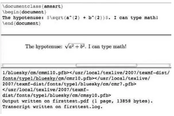
1. A text editor is used to create a LATEX source file. A source file might look like the top window in Figure 1.1:
\documentclass{amsart} \begin{document}
The hypotenuse: $\sqrt{a^{2} + b^{2}}$. I can type math! \end{document}
Note that the source file is different from a typical word processor file. All characters are displayed in the same font and size.
2. Your friend “typesets” the source file(tells the application to produce a typeset ver-sion)and views the result on the monitor(the two corners indicate material typeset by LATEX):
as in the middle window in Figure 1.1.
3. The editing cycle continues.Your friend goes back and forth between the source file and the typeset version, making changes and observing the results of these changes.
4. The file is printed. Once the typeset version is satisfactory, it is printed, creating a paper version of the typeset article. Alternatively, your friend creates a PDFfile of the typeset version (see Chapter 13.1.2).
If LATEX finds a mistake when typesetting the source file, it opens a new window,
thelogwindow,illustrated as the bottom window in Figure 1.1, and displays an error message. The same message is saved into a file, called thelogfile. Look at the figures in Appendix A, depicting a variety of editing windows, windows for the typeset article, andlogwindows for the two LATEX implementations discussed there.
Various LATEX implementations have different names for the source file, the text
editor, the typeset file, the typeset window, thelogwindow, and thelogfile. Become familiar with these names for the LATEX implementation you use, so you can follow
along with our discussions. In Appendix A, we bring you up to speed for the LATEX
implementations discussed therein.
1.4
Three productivity tools
Most LATEX implementations have these important productivity tools:
Synchronization To move quickly between the source file and the typeset file, most
LATEX implementations offersynchronization, the ability to jump from the typeset
file to the corresponding place in the source file and from the source file to the corresponding place in the typeset file.
Block comment Block comments are very useful:
1. When looking for a LATEX error, you may want LATEX to ignore a block of text
in the source file (see page 51).
2. Often you may want to make comments about your project but not have them printed or you may want to keep text on hand while you try a different op-tion. To accomplish this, insert a comment character,%, at the start of each line where the text appears. These lines are ignored when the LATEX file is
processed.
Select a number of lines in a source document, then by choosing a menu option all the lines (the whole block) are commented out (a%sign is placed at the beginning of each line). This isblock comment. The reverse isblock uncomment.
Jump to a line This is specified by the line number in the source file. To find an error,
LATEX suggests that you jump to a line.
Find out how your LATEX implements these features. In Appendix A, we discuss
how these features are implemented for the LATEX we install.
Pay careful attention how your LATEX implementation works. This enables you to
2
Typing text
In this chapter, I introduce you to typesetting text by working through examples. More details are provided throughout the book, in particular, in Chapters 5 and 6.
A source file is made up oftext, math(formulas), andinstructions(commands)
toLATEX. For instance, consider the following variant of the first sentence of this
para-graph:
A source file is made up of text, math (e.g., $\sqrt{5}$), and \emph{instructions to} \LaTeX.
This typesets as
A source file is made up of text, math (e.g.,√5), andinstructions to LATEX.
In this sentence, the first part
A source file is made up of text, math (e.g.,
is text. Then
is math
), and
is text again. Finally,
\emph{instructions to} \LaTeX.
are instructions. The instruction\emph is acommand with an argument, while the instruction\LaTeXis acommand without an argument.
Commands, as a rule, start with a backslash (\) and tell LATEX to do something
special. In this case, the command\emphemphasizes itsargument(the text between the braces). Another kind of instruction to LATEX is called anenvironment.For instance,
the commands
\begin{flushright}
and
\end{flushright}
enclose aflushrightenvironment; thecontent, that is, the text that is typed between these two commands, is right justified (lined up against the right margin) when type-set. (Theflushleftenvironment creates left justified text; thecenterenvironment creates text that is centered horizontally on the page.)
In practice, text, math, and instructions (commands) are mixed. For example,
My first integral: $\int \zeta^{2}(x) \, dx$.
is a mixture of all three; it typesets as
My first integral: Rζ2(x)dx.
Creating a document in LATEX requires that we type the text and math in the source
file. So we start with the keyboard, proceed to type a short note, and learn some simple rules for typing text in LATEX.
2.1
The keyboard
The following keys are used to type text in a source file:
You may also use the following punctuation marks:
, ; . ? ! : ‘ ’
-and the space bar, the Tab key, -and the Return (or Enter) key.
Since TEX source files are “pure text” (ASCIIfiles), they are very portable. There is one possible problem limiting this portability, the line endings used in the source file. When you press the Return key, your text editor writes an invisible code into your source file that indicates where the line ends. Since this code may be different on different platforms (PC, Mac, andUNIX), you may have problems reading a source file created on a different platform. Luckily, many text editors include the ability to switch end-of-line codes and some, including the editors inWinEdtandTeXShop, do so automatically.
Finally, there are thirteen special keys that are mostly used in LATEX commands:
# $ % & ~ _ ^ \ { } @ " |
If you need to have these characters typeset in your document, there are commands to produce them. For instance,$is typed as\$, the underscore, , is typed as\_, and % is typed as \%. Only @requires no special command, type @to print@. There are also commands to produce composite characters, such as accented characters, for example¨a, which is typed as\"{a}. See Section 5.4.4 for a complete discussion of symbols not available directly from the keyboard and Appendix C for the text sym-bol tables. Appendices B and C are reproduced in thesamplesfolder as aPDF file, SymbolTables.pdf.
LATEX prohibits the use of other keys on your keyboard—unless you are using a
version of LATEX that is set up to work with non-English languages (see Appendix G).
When trying to typeset a source file that contains a prohibited character, LATEX displays
an error message similar to the following:
! Text line contains an invalid character. l.222 completely irreducible^^?
^^?
In this message,l.222means line 222 of your source file. You must edit that line to remove the character that LATEX cannot understand. Thelogfile (see Section D.3.4)
also contains this message. For more about LATEX error messages, see Sections 3.2
and 4.3.1.
2.2
Your first note
We start our discussion on how to type a note in LATEX with a simple example. Suppose
It is of some concern to me that the terminology used in multi-section math courses is not uniform.
In several sections of the course on matrix theory, the term “hamiltonian-reduced” is used. I, personally, would rather call these “hyper-simple”. I invite others to comment on this problem.
Of special concern to me is the terminology in the course by Prof. Rudi Hochschwabauer. Since his field is new, there is no accepted terminology. It is imperative that we arrive at a satisfactory solution.
To produce this typeset document, create a new file in yourworkfolder with the namenote1.tex. Type the following, including the spacing and linebreaks shown, but not the line numbers:
1 % Sample file: note1.tex 2 \documentclass{sample} 3
4 \begin{document}
5 It is of some concern to me that 6 the terminology used in multi-section 7 math courses is not uniform.
8
9 In several sections of the course on 10 matrix theory, the term
11 ‘‘hamiltonian-reduced’’ is used. 12 I, personally, would rather call these 13 ‘‘hyper-simple’’. I invite others 14 to comment on this problem. 15
16 Of special concern to me is the terminology 17 in the course by Prof.~Rudi Hochschwabauer. 18 Since his field is new, there is no accepted 19 terminology. It is imperative
20 that we arrive at a satisfactory solution. 21 \end{document}
Alternatively, copy thenote1.texfile from thesamplesfolder (see page 4). Make sure thatsample.clsis in yourworkfolder.
The first line ofnote1.texstarts with%. Such lines are calledcommentsand are ignored by LATEX. Commenting is very useful. For example, if you want to add
simply put, we believe % actually, it’s not so simple
Everything on the line after the%character is ignored by LATEX.
Line 2 specifies thedocument class(in our case,sample)1 that controls how the
document is formatted.
The text of the note is typed within thedocumentenvironment, that is, between the lines
\begin{document}
and
\end{document}
Now typesetnote1.tex. If you useWinEdt, click on theTeXifyicon. If you use TeXShop, click theTypesetbutton. You should get the typeset document as shown on page 10. As you can see from this example, LATEX is different from a word processor.
It disregards the way you input and position the text, and follows only the formatting instructions given by the markup commands. LATEX notices when you put a blank space
in the text, but it ignoreshow many blank spaceshave been inserted. LATEX does not
distinguish between a blank space (hitting the space bar), a tab (hitting the Tab key), and asinglecarriage return (hitting Return once). However, hitting Return twice gives a blank line;one or moreblank lines mark the end of a paragraph.
LATEX, by default, fully justifies text by placing a flexible amount of space
be-tween words—the interword space—and a somewhat larger space between senten-ces—theintersentence space. If you have to force an interword space, you can use the \ command (in LATEX books, we use the symbol to mean a blank space). See
Sec-tion 5.2.2 for a full discussion.
The ~ (tilde) command also forces an interword space, but with a difference; it keeps the words on the same line. This command is called atieor nonbreakable space(see Section 5.4.3).
Note that on lines 11 and 13, the left double quotes are typed as‘‘ (two left single quotes) and the right double quotes are typed as’’(two right single quotes or apostrophes). The left single quote key is not always easy to find. On an American keyboard,2it is usually hidden in the upper-left or upper-right corner of the keyboard,
and shares a key with the tilde (~).
1I know you have never heard of thesampledocument class. It is a special class created for these
exercises. You can find it in thesamplesfolder (see page 4). If you have not yet copied it over to thework folder, do so now.
2The location of special keys on the keyboard depends on the country where the computer was sold. It
2.3
Lines too wide
LATEX reads the text in the source file one line at a time and when the end of a paragraph
is reached, LATEX typesets the entire paragraph. Occasionally, LATEX gets into trouble
when trying to split the paragraph into typeset lines. To illustrate this situation, modify
note1.tex. In the second sentence, replacetermbystrange termand in the fourth
sentence, delete Rudi , including the blank space following Rudi. Now save this
modified file in yourwork folder using the name note1b.tex. You can also find
note1b.texin thesamplesfolder (see page 4).
Typesettingnote1b.tex, you obtain the following:
It is of some concern to me that the terminology used in multi-section math courses is not uniform.
In several sections of the course on matrix theory, the strange term “hamiltonian-reduced” is used. I, personally, would rather call these “hyper-simple”. I invite others to comment on this problem.
Of special concern to me is the terminology in the course by Prof. Hochschwabauer. Since his field is new, there is no accepted terminology. It is imperative that we arrive at a satisfactory solution.
The first line of paragraph two is about1/4inch too wide. The first line of
para-graph three is even wider. In thelogwindow, LATEX displays the following messages:
Overfull \hbox (15.38948pt
too wide) in paragraph at lines 9--15 []\OT1/cmr/m/n/10 In sev-eral sec-tions of the course on ma-trix the-ory, the strange term
‘‘hamiltonian-Overfull \hbox (23.27834pt too wide) in paragraph at lines 16--21
[]\OT1/cmr/m/n/10 Of spe-cial con-cern to me is the ter-mi-nol-ogy in the course by Prof. Hochschwabauer.
You will find the same messages in thelogfile (see Sections 1.3 and D.2.1).
The first message,
Overfull \hbox (15.38948pt too wide) in paragraph at lines 9--15
refers to the second paragraph (lines 9–15 in the source file—its location in the typeset document is not specified). The typeset version of this paragraph has a line that is
15.38948 points too wide. LATEX usespoints(pt) to measure distances; there are about
The next two lines,
[]\OT1/cmr/m/n/10 In sev-eral sec-tions of the course on ma-trix
the-ory, the strange term
‘‘hamiltonian-identify the source of the problem: LATEX did not properly hyphenate the word
hamiltonian-reduced
because it (automatically) hyphenates a hyphenated wordonly at the hyphen.
The second reference,
Overfull \hbox (23.27834pt too wide) in paragraph at lines 16--21
is to the third paragraph (lines 16–21 of the source file). There is a problem with the wordHochschwabauer; LATEX’s standard hyphenation routine cannot handle it (a
Ger-man hyphenation routine would have no difficulty hyphenating this name—see Ap-pendix G). If you encounter such a problem, you can either try to reword the sentence or insert one or moreoptional(or discretionary)hyphen commands(\-), which tell LATEX
where it may hyphenate the word. In this case, you can rewriteHochschwabaueras Hoch\-schwa\-bauerand the second hyphenation problem disappears. You can also utilize the\hyphenationcommand (see Section 5.4.9).
Sometimes a small horizontal overflow can be difficult to spot. Thedraft ument class option may help (see Sections 11.5, 12.1.2, and 18.1 for more about doc-ument class options). LATEX places a black box (orslug) in the margin to mark an
overfull line. You can invoke this option by changing the\documentclassline to \documentclass[draft]{sample}
A version ofnote1b.tex with this option can be found in thesamplesfolder under the namenoteslug.tex. Typeset it to see the “slugs”.
2.4
More text features
Next, we produce the following note:
September 12, 2006
From the desk of George Gr¨atzer
Type in the source file, without the line numbers. Save it asnote2.texin your workfolder (note2.texcan be found in thesamplesfolder—see page 4):
1 % Sample file: note2.tex 2 \documentclass{sample} 3
4 \begin{document} 5 \begin{flushright}
6 \today
7 \end{flushright}
8 \textbf{From the desk of George Gr\"{a}tzer}\\[22pt] 9 October~7--21 \emph{please} use my
10 temporary e-mail address: 11 \begin{center}
12 \texttt{George\[email protected]} 13 \end{center}
14 \end{document}
This note introduces several additional text features of LATEX:
The\todaycommand (in line 6) to display the date on which the document is typeset (so you will see a date different from the date shown above in your own typeset document).
The environments toright justify(lines 5–7) andcenter(lines 11-13) text.
The commands to change the text style, including the\emphcommand (line 8) to
emphasizetext, the\textbfcommand (line 9) forboldtext, and the\texttt com-mand (line 12) to producetypewriter styletext.
These arecommands with arguments. In each case, the argument of the com-mand follows the name of the comcom-mand and is typed between braces, that is, between {and}.
The form of the LATEX commands: Almost all LATEXcommandsstart with a backslash
(\) followed by the command name. For instance, \textbf is a command and textbfis the command name. The command name is terminated by the first non-alphabetic character, that is, by any character other than a–z or A–Z. Sotextbf1is not a command name, in fact,\textbf1typesets as1. (Let us look at this a bit more closely. \textbfis a valid command. If a command needs an argument and is not followed by braces, then it takes the next character as its argument. So\textbf1is the command\textbfwith the argument1, which typesets as bold1:1.) Note that command names arecase sensitive.Typing\Textbfor\TEXTBFgenerates an error message.
dash. Use triple hyphens for theem dashpunctuation mark—such as the one in this sentence.
Thenew linecommand,\\(or\newline): To create additional space between lines (as in the last note, under the lineFrom the desk. . .), you can use the\\command and specify an appropriate amount of vertical space:\\[22pt]. Note that this com-mand usessquare bracketsrather than braces because the argument isoptional.The distance may be given in points (pt), centimeters (cm), or inches (in). (There is an analogousnew pagecommand,\newpage, not used in this short note.)
Special rules for special characters (see Section 2.1), foraccented charactersand for someEuropean characters.For instance, the accented character¨ais typed as\"{a}. Accents are explained in Section 5.4.7 (see also the tables in Section C.2).
3
Typing math
While marking up text in LATEX is easy, marking up math is less intuitive because
math formulas are two-dimensional constructs and we have to mark them up with a one-dimensional string of characters. However, even the most complicated two-dimensional formula is made up of fairly simple building blocks. So by concentrating on the building blocks—selectively, just learn the ones you need—you can get started with math quickly.
3.1
A note with math
In addition to the regular text keys and the 13 special keys discussed in Section 2.1, two more keys are used to type math:
< >
The formula2 <|x|> y(typed as$2 < |x| >y$) uses both. Note that such math formulas, calledinline, are enclosed by$symbols. We discuss shortly another kind of math formula calleddisplayed.
In first-year calculus, we define intervals such as (u, v) and (u,∞). Such an interval is aneighborhood ofaifais in the interval. Students should realize that
∞is only a symbol, not a number. This is important since we soon introduce concepts such as limx→∞f(x).
When we introduce the derivative
lim
x→a
f(x)−f(a)
x−a ,
we assume that the function is defined and continuous in a neighborhood ofa.
To create the source file for this mixed text and math note, create a new document with your text editor. Name itmath.tex, place it in theworkfolder, and type in the following source file—without the line numbers—or simply copymath.texfrom the samplesfolder (see page 4):
1 % Sample file: math.tex 2 \documentclass{sample} 3
4 \begin{document}
5 In first-year calculus, we define intervals such 6 as $(u, v)$ and $(u, \infty)$. Such an interval 7 is a \emph{neighborhood} of $a$
8 if $a$ is in the interval. Students should 9 realize that $\infty$ is only a
10 symbol, not a number. This is important since 11 we soon introduce concepts
12 such as $\lim_{x \to \infty} f(x)$. 13
14 When we introduce the derivative 15 \[
16 \lim_{x \to a} \frac{f(x) - f(a)}{x - a}, 17 \]
18 we assume that the function is defined and 19 continuous in a neighborhood of $a$. 20 \end{document}
This note introduces several basic concepts of math in LATEX:
There are two kinds of math formulas and environments inmath.tex:
– Inlinemath environments open and close with$(as seen throughout this book) or open with\(and close with\).
Within math environments, LATEX uses its own spacing rules and completely ignores
the white space you type, with two exceptions:
– Spaces that terminate commands. So in$\infty a$ the space is not ignored, $\inftya$produces an error.
– Spaces in the arguments of commands that temporarily revert to regular text. \textis such a command (see Sections 3.3 and 7.4.6).
The white space that you add when typing math is important only for the readability of the source file. We summarize with a simple rule.
Rule
Spacing in text and mathMany spaces equal one space in text, whereas your spacing is ignored in math, unless the space terminates a command.
A math symbol is invoked by a command. For example, the command for∞is \inftyand the command for→is\to. The math symbols are organized into tables in Appendix B (see alsoSymbolTables.pdfin thesamplesfolder).
Some commands, such as\sqrt, needargumentsenclosed by{and}. To typeset
√
5, type$\sqrt{5}$, where\sqrtis the command and5is the argument. Some commands need more than one argument. To get
3 +x
5 type
\[
\frac{3+x}{5} \]
where\fracis the command,3+xand5are the arguments—we indent for readabil-ity.
3.2
Errors in math
Even in such a simple note there are opportunities for errors. To help familiarize your-self with some of the most commonly seen LATEX math errors and their causes, we
deliberately introduce mistakes intomath.tex. The version ofmath.texwith mis-takes ismathb.tex. By inserting and deleting%signs, you make the mistakes visible to LATEX one at a time—recall that lines starting with%are comments and are therefore