Modeling urban traffic noise with stochastic and deterministic traffic models
Alberto Ramírez
⇑, Efraín Domínguez
Facultad de Estudios Ambientales y Rurales, Pontificia Universidad Javeriana, Transversal 4, No. 42-00, Piso 8, Bogotá, Colombia
a r t i c l e
i n f o
Article history:
Received 27 January 2012
Received in revised form 6 June 2012 Accepted 1 August 2012
Available online 3 September 2012
Keywords: Noise pollution Urban modeling
Traffic noise prediction model Traffic dynamics
Urban noise monitoring
a b s t r a c t
This paper presents the development and evaluation of a stochastic dynamic traffic noise prediction model based on noise curves for vehicle classes and their speed. The model was tested on urban two-lane roads in the city of Bogotá and was established on the basis of the fit of singleLi,17secnoise functions for different types of vehicles. The model showed a slightly better fit than was found in four deterministic models that are highly internationally recognized. Additionally, a deterministic model was derived con-textualized to the city of Bogotá. The approach used is promising for further investigations of urban traffic noise given the traffic conditions in these systems.
Ó2012 Elsevier Ltd. All rights reserved.
1. Introduction
Urban noise pollution is causing increased health risks in the population. This is due both to the fact that noise levels, particu-larly those associated with transport, have increased dramatically since the mid-twentieth century and that a higher percentage of the world population is now concentrated in urban systems[1,2]. This problem has also increased economic costs due to failing health and reduced productivity of the population, affecting be-tween 0.2% and 2% of gross domestic product in the US [3]. In the European Union, the costs range between $13 billion and $38 billion per year[4]. In addition, traffic noise causes the depre-ciation of properties exposed to high noise levels[5].
Studies on urban noise are becoming more numerous, reflecting the growing importance of this pollutant, for which levels cur-rently exceed those specified by regulations in Spain[6], Iran[7], India[8], Egypt[9], China[10], Brazil[11]and Colombia[12,13], among others.
Computer models are highly valued in developed countries for assessing environmental problems, including sources of pollution, their spreading in the environment, impacts on human populations and associated regulatory processes, many of which follow the guidelines of the USEPA[14]. Modeling of traffic noise represents an example of this technique and has been implemented in the context of environmental impact studies for transport projects
[15]. Additionally, this type of modeling has played an important role in the analysis of mitigation measures during road construc-tion[16,17]and in identifying the variables with the highest noise
incidence[9,18]. Noise prediction also plays a prominent role in planning and development of new urban projects and roads[16].
The traffic noise model plays an important role in the construc-tion of noise maps, since they combine both observed and simu-lated records. These maps have been employed mainly for urban planning, environmental risk assessment [19], identification of hotspots, evaluation of the exposed population and simulation of mitigation measures[20,21].
The simplest models have been designed based on relationships between the logarithm of the number of vehicles and the level of noise they generate [7,22–24]. The relationship between these two variables is obvious, as the greater the number of vehicles that are simultaneously on the road, the greater the number of emis-sions sources there will be. More elaborate models have also in-cluded the proportion of heavy vehicles and speed, and even variables such as pavement type, width and inclination of the track and height of buildings, among others[7,15,23,25–30].
These models are based on theoretical factors that are applica-ble based on statistical relationships and on macroscopic traffic variables such as total flow and average speed. Their results have been very good related to roads and highways where traffic pre-vails, and flow conditions are relatively homogeneous[9,16,17]. In contrast, these same models have rarely been applied to urban roads where traffic volumes and speeds are not fixed due to the start-stop and acceleration–deceleration situations that are typical of these systems[5]and because of cycles in traffic and noise asso-ciated with traffic lights[13,31].
Nevertheless, research on urban intersections has achieved a good fit between the continuous equivalent level, (Leq), and the traffic volume, the number of heavy vehicles, the slope and the type of pavement[32].
0003-682X/$ - see front matterÓ2012 Elsevier Ltd. All rights reserved.
http://dx.doi.org/10.1016/j.apacoust.2012.08.001
⇑Corresponding author. Tel.: +57 1 3208320x4819; fax: +57 1 3208320x4859. E-mail address:[email protected](A. Ramírez).
Contents lists available atSciVerse ScienceDirect
Applied Acoustics
Other mathematical approaches that have achieved good per-formance include neural networks [33,34], microscopic traffic models[35,36]and models based on single traffic noise[37].
In Colombia, the problem of traffic noise has been largely over-looked by environmental authorities. Very few studies have in-volved modeling, and their results have been highly variable
[12,13,38,39]. This report presents the results of a study in which a stochastic and dynamic microscopic model is developed, and its performance is analyzed in the city of Bogotá based on the sin-gle noise generated by each vehicle during its passage in front of a measurement point. Additionally, we compare the results of this model with a deterministic model derived from it, as well as four international deterministic models that are widely used.
2. Methodology
2.1. Single noise
This study was conducted in Bogota. As a starting point, vehicles were classified into the following categories: motorcycles, cars (including cars, trucks, small delivery vans and microbuses), buses, mini-buses (small buses) and trucks (over 3 tons). Subsequently, we conducted measurements of single noise on the streets of the city (n= 533 vehicles), seeking to exclude the impact of other vehi-cles and other sources of noise. To this end, we used an integrated Extech type II sound level meter (SLM) to evaluate the instanta-neous sound level (Li,1sec) during the approach and passage of each vehicle in front of the SLM on roads with 1 and 2 lanes. These mea-surements followed conventional techniques[15]and were con-ducted using a tripod and a windscreen at a height of 1.2 m at a distance of 1 m from the road with A and slow weights. In parallel, we measured the speed at which each vehicle was traveling using manual Bushnell equipment. In all cases, the prevailing conditions included flat, dry roads, wind speeds less than 4 km/h and a low incidence of other noise sources.
For each type of vehicle, we conducted a regression analysis be-tween the maximum noise level (when passing in front of the SLM) and speed. Because this yielded low coefficients of determination, we implemented classification trees to dissociate subgroups depending on the speed of vehicles. Subsequently, we averaged all noise levels recorded in each subgroup at time zero (passing in front of the SLM) and during the approach at times1 through8 s in time steps of 1 s. Using these values, we tested various models of lin-ear and nonlinlin-ear regression and chose the model with the highest coefficient of determination using SPSS v.15 (statistical software) and Curve Expert v.1.3 (nonlinear regression). The noise level was assumed to be symmetric for the approach and retreat of vehicles.
2.2. Stochastic model
Based on this information, we built a dynamic model using the Stella v.8 program (dynamic modeling software) consisting of 3 segments:
i. A stochastic Monte Carlo traffic simulator for each lane, with sampling without replacement, which defines for each sec-ond whether or not a vehicle is present and the class to which it belongs, along with its speed simulated from a nor-mal distribution with estimated parameters (l,
r
2) for each vehicle class and station. In this regard, the model follows the guidelines given by the[5]regarding including specific conditions for each lane.ii. A time window of 17 s (8. . .0. . .+8) for each lane, in
which the vehicle is moving and sends information about instantaneous sound pressure (Li;1sec) from the Weibull func-tions estimated from vehicle type and speed.
iii. A collection point for the information, which receives the instantaneous sound pressure of the two lanes every second and calculates the continuous equivalent level (Eqs.(1) and (2)). This descriptor is the constant sound level over a stated period of time which is equivalent in total sound energy to the time-varying sound level measured over the same period of time and is used worldwide in traffic noise evaluation
[15,26]. The simulation and sampling time was 10 min, which is a duration that was previously shown (presam-pling) to be sufficient forLAeqstabilization. This unit of time was reported as suitable for such measurements[35].
Calculation of the continuous equivalent level for each lane was determined as follows:
The model is dynamic and is based on the physical principle of the addition of sound pressure per vehicle and lane, along with empirical equations for single noise based on speed and vehicle type, which in this case, correspond to the Weibull function. The model also incorporates randomness derived from the speed of each vehicle, which is why the continuous equivalent level estimated at each station was obtained from the average of 10 simulations.
The assumptions included in the model were as follows: (a) conservation of vehicles during the 17-s window; (b) sound energy conservation, but with divergence based on the distance between the vehicle and the level meter, which is implied in the Weibull function; (c) constant vehicle speed during passage through the time window; (d) no vehicle passing any other vehicle or changing lanes; (e) negligible effects of reflection due to walls, reflection and shielding between vehicles and refraction and absorption by other elements present in the acoustic field; (f) negligible impacts of other noise sources compared to the sound pressure arising from the vehicle; and (g) the climatic impact is considered negligible gi-ven the distance.
2.3. Deterministic models
For comparison purposes, we evaluated the German model RLS90 – Richtlinien für den Lärmschutz an Straben[25]; the Eng-lish model CoRTN – Calculation of road traffic noise[40]; the Nor-dic model NorNor-dic preNor-diction method for road traffic noise-statens planverk 96[25,41]and the Northamerican model TNM – Traffic noise model V.2.5 [27]. Previous models estimate theLeq based on traffic flow, speed and heavy vehicle proportion. They are static and deterministic.
We also derived and evaluated a deterministic model based on the TNM, but operating with the single noise levels measured in Bogotá (Eq.(3)).
LAeq;17segðMotorcycles;sÞ
whereQj,sis number of vehicles of typej, at speeds;LAeq,17seg,j,sis 17 s continuous equivalent level for vehiclej, at speeds.
2.4. Sampling stations
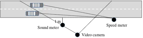
We studied 28 two-lane stations (one- and two-way streets) in the city of Bogotá. These stations were chosen because they exhib-ited a low noise level associated with sources other than the vehi-cles being studied and were located in contexts that varied with respect to volume, composition and vehicle speed. At each station, the following descriptors were recorded: (a) continuous equivalent level for 10 min (LAeq,10min.), measured with an integrated Extech type II sound level meter at a height of 1.2 m, located 1 m of from the lane and more than 4 m from any facades; (b) the number of vehicles of each type in each lane, which were video recorded; (c) the speed of as many vehicles as possible, recorded using a Bushnell speedometer; and (d) the distance between the sound le-vel meter and the middle of the lanes, to correct for the divergence of the deterministic models (Fig. 1).
Sampling points were chosen more than 50 m away from traffic lights to reduce stop-start effects during sampling but there were numerous situations of detention.
2.5. Analysis
2.5.1. Deterministic models
The English, German and Nordic models were calculated using a Java algorithm, while the US model of the Federal Highway Admin-istration was computed from the Traffic Noise Model software V 2.5. The results were all corrected by adding background noise –
L90– and adjusting distance of each lane to the sound level meter (Eq.(4), ford= 1)[37]:
whereLis sound pressure at a specific distanceD
;LRef.is sound pressure at a reference distanceDRef.
To evaluate the models performance, we divided the total sam-ple into 2 groups: 20 samsam-ples for estimation and calibration and 8 samples for validation. Calibration was performed by adjusting the parameters of the models up to 50% of its value, based on the func-tion that minimizes the differences between observed and esti-mated results. This procedure was performed with the solver
function of Excel. A similar method was employed by Alimoham-madi et al.[7]and by Calixto et al.[11].
2.5.2. Stochastic model
We estimated the continuous equivalent level through the Stel-la model for each station from the average of 10 simuStel-lations. In addition, regression analysis between the background-noise and mean error – ME – (Eq.(5)) was carried out to establish whether there was incidence of the first variable in the second. This analysis was necessary as background noise was not added explicitly in the stochastic model as was done in the deterministic models. We did not find, however, a relationship between them (p> 0.05).
The deterministic model derived from the stochastic model was calibrated allowing variations up to 5% in theLAeq,17sof each type of vehicle, following a similar procedure to that described previously for the deterministic model (Table 1).
We studied the goodness of fit of the models using parameters that relate the measured and estimated values, such as themean error(ME), themean absolute error(MAE), themean absolute rela-tive error (MARE) and the coefficient of determination (r2) (Eqs.
(5)–(8))[42].
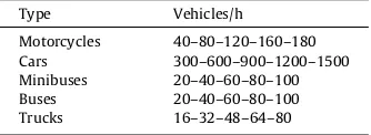
Likewise, for the microscopic model, we conducted a sensitivity analysis that evaluated the noise level at all stations under varying traffic volumes. To this end, we rounded the maximum value of each vehicle type and divided it into five equal units. Subsequently, we simulatedLAeq,10minfor each station using the values given in Table 2. Given the high sound pressure levels found in the city, this analysis favored an approach that reduced the number of vehicles and did not take into account variations in density and velocity re-ferred to in the fundamental traffic diagram[43].
The procedure of the research is summarized inFig. 2.
3. Application and discussion
3.1. Traffic conditions
The traffic conditions for the 28 samples are presented inTable 3, highlighting the dominance of cars over other types of vehicles.
3.2. Single noise
The number of vehicles tested in each class to obtain the single sound level varied between 30 and 115 (n= 533 vehicles). The best
1 m Sound meter
Video camera
Speed meter
Fig. 1.Information recorded in field:LAeq,10min, speed of different types of vehicles
in different lanes, video recording for vehicles count per lane.
Table 1
Calibration of singleLAeq,17secfor the stochastic model.
LAeq,17secestimated LAeq,17secadjusted
Lane 1 2 1 2
MotorcyclesL1647 63.5 66.7
MotorcyclesL1 47–70 66.3 69.7
MotorcyclesL1 > 70 71.1 71.1
MotorcyclesL2651 62.7 65.7
MotorcyclesL2 > 51 67.3 65.5
CarsL1650 63.7 62.2
MinibusesL1 > 54 71.9 68.7
MinibusesL2 71.9 72.2
Buses 74.9 74.2 75.3 77.3
Trucks 75.6 74.8 74.7 75.2
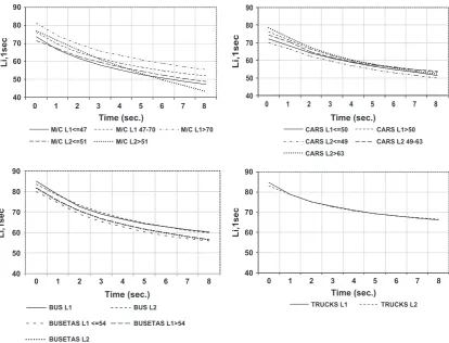
function to describe the relationship between the average instanta-neous sound pressure and the approach of the vehicle in a 9-s win-dow was the Weibull function (Eq.(9)). For all types of vehicles, the coefficient of determination was greater than 0.990 (n= 9,
p< 0.001), and function parameters varied as follows:abetween 71.9 and 84.9, bbetween 44.8 and 123.6, c between 2 and 3.4 anddbetween0.6 and0.3 (Fig. 3).
Li;1s¼abect
d
ð9Þ
Similar plots were obtained by[37], who measuredLAeq,10secand also found a weak relationship between the speed and the sound pressure within each vehicle class, which indicates high variability within the classes.
3.3. Modeling
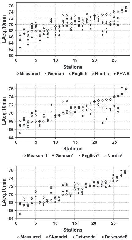
The performance of the models across the different metrics is shown inTable 4 and Figs. 4 and 5. From this, we extract the following:
i. The stochastic model and the deterministic model derived from it, showed better performance than the deterministic models. The mean absolute error –MAE- of the stochastic model was close to 1 dBA, while the MAE of the determinis-tic models is between 1.7 and 3.6 dBA.
ii. The mean error – ME – of the stochastic model is slightly negative which indicates a small overestimation in the model output, whereas it was positive for the deterministic models. However, the ME was lower in the Nordic model, which due to its value near zero, indicates a lack of bias. iii. All of the adjusted deterministic models resulted in a better
fit than in the original models. However, there were no significant differences in the average residuals (p> 0.05).
iv. The goodness-of-fit statistics of all models in the first 20 sta-tions (calibration) was better than in the last 8 stasta-tions (val-idation); the stochastic model adjustment back 0.5 dBA and the deterministic models 1–2 dBA, nevertheless, stochastic model performance remains high. The discrepancy possibly occurred by significant changes in traffic conditions, because in the last 8 seasons the average volume of buses and mini-buses was double that of the first 20 stations and the speed of the cars was 1.8 times higher.
The underestimation ofLAeqby the macroscopic models could be a sign that single noise in the city of Bogotá is higher than in other countries.
The results of other studies show similar or slightly lower mod-els performance than was obtained in this study. In Beirut, there was an underestimation of 5 dBA using the FHWA model, which could be caused by the impact of background noise, specific char-acteristics of different forms of transportation, the use of horns or excessive acceleration or deceleration; however, with the adjusted model, the differences were reduced to 0.7–1.2 dBA[27]. Further-more, the FHWA model was tested previously in Bogota, where it presented an underestimation of 7 dBA (close to 10%), which the authors attributed to the possible effect of background noise
[39], although the results of the present study suggest that under-estimation arises from the high level of noise produced by single buses and minibuses.
The CoRTN model was applied in Tehran (Iran), where it exhib-ited an overestimation of L10, 1hof 1.46 dBA, which appeared to be related to traffic fluctuations and differences between classes of vehicles and types of surfaces[7]. In Dublin, with this same model, there were errors of up to 3 dB and underestimations of up to1.8 dB, amounts considered by the authors as adequate for map-ping and simulate noise mitigation measures [20]. Likewise, in Hong Kong there were errors of up to 3 dB for 90% of the simulated Table 2
Traffic flow used in the sensitivity analysis of the stochastic model (observed maximum flow divided into 5 classes).
Type Vehicles/h
Motorcycles 40–80–120–160–180 Cars 300–600–900–1200–1500 Minibuses 20–40–60–80–100
Buses 20–40–60–80–100
Trucks 16–32–48–64–80
-8 -7 -6 -5 -4 -3 -2 -1 0 1 2 3 4 5 6 7 8
Leq estimated
L1s
Leq measured
R2, a , b - ME - MAE - MARE
Time window: 17 seconds Volume and
composition
Average speed and
standard deviation
Monte Carlo simulation: vehicle type, sample without replacement
Normal distribution simulation: speed (µ, σ)
Weibull function for vehicle type
Leq estimated
Stochastic model
Deterministic models
Fig. 2.Research methodology. Table 3
Range observed for the main traffic characteristics.
Motorcycles Cars Minibuses Buses Trucks
Volume (No./10 min)
Lowest 3 49 0 0 0
Highest 36 247 36 7 13
Speed (km/h)
Lowest 20 10 22 10 25
data[44]. The same model was used in Pereira (Colombia), where it presented an average error of 1.62 dBA forL10,1h[38].
In the countries of origin of the Nordic model, it has shown er-rors near ±2 dBA at a distance of 200 m[41]. In Japan, it presented differences of less than 1 dB in areas without buildings and up to 4 dBA in developed areas[17].
The German model was employed in the city of Curitiba (Brazil), where it yielded a MARE between 2.2% and 2.9%[11], which repre-sents approximately 1.6–2.1 dBA. This same model tested in the city of Chungiu (Republic of Korea) gave a ME of 0.6 dB and anr2
of 0.50[45].
In general, the reported errors meet the requirements of gov-ernment regulations and road engineers[23], however, caution is to be exercised since the presence of anomalous traffic noise events can affect the results up to 4 dB[46].
For the previously reported European models, Arana et al.[25]
found that there are differences in the parameters that define the
sound pressure of heavy vehicles. The German model penalizes these vehicles the most and the Nordic model the least. For exam-ple, in the German model, the sound pressure of a heavy vehicle is equivalent to 20 times that of a light one. In contrast, in the English model, it is between 4.5 and 14 times that of a light one, and in the Nordic model, it is considered to be between 6 and 10 times that of a light one, depending on the speed. However, this variable is likely to not have played a relevant role in the present study because of the low flow of these vehicles.
Compared to neural network technology, the results associated with our model are not considerably different. Cammarata et al.
[33]accepted errors of up to 2.5 dBA during the training phase of network implementation. Genaro et al.[34]incorporated 26 input variables and achieved errors that were generally less than 5%, with a prominent average error of 0.79 dBA.
For micromodels, Can et al.[35]believe that the incorporation of simple macroscopic rules may be sufficient to achieve reason-able estimates of city traffic noise. They found that this noise is more sensitive to traffic signals than to the driving conditions. However, application of a micromodel in the city of Gentbrugge (Belgium) showed errors of less than 3 dBA, with the greatest dif-ferences being observed under conditions of low traffic density
[36].
As noted previously, the fit of the stochastic model developed in this study gives slightly better results than those obtained in other studies, which is explained by the fact that our model considered contextual information specific to Bogota, where buses and mini-buses emit high levels of single noise. In this sense, from a physical perspective, both the stochastic model and the deterministic mod-el devmod-eloped here are equivalent to the FHWA modmod-el, which is based on combining single traffic noise. This bestows upon it a 40
50 60 70 80 90
Li,1sec
Time (sec.)
M/C L1<=47 M/C L1 47-70 M/C L1>70
M/C L2<=51 M/C L2>51
40 50 60 70 80 90
Li,1sec
Time (sec.)
CARS L1<=50 CARS L1>50
CARS L2<=49 CARS L2 49-63
CARS L2>63
40 50 60 70 80 90
0 1 2 3 4 5 6 7 8 0 1 2 3 4 5 6 7 8
2
0 1 3 4 5 6 7 8
Li,1sec
Time (sec.)
TRUCKS L1 TRUCKS L2 40
50 60 70 80 90
0 1 2 3 4 5 6 7 8
Li,1sec
Time (sec.)
BUS L1 BUS L2
BUSETAS L1 <=54 BUSETAS L1>54
BUSETAS L2
Fig. 3.Li,1sec.curves (Weibull function) for different vehicles subclasses at different speeds approach (M/C: Motorcycles;L: Lane; speed: km/h).
Table 4
Performance of all models under different metrics (St: stochastic; Det: deterministic derived;: adjusted parameters).
r2 ME MAE MARE
St-model 0.742 0.51 1.14 0.016
Det-model 0.756 0.33 1.09 0.016
Det-model 0.868
0.09 0.76 0.011
German 0.425 1.53 2.09 0.029
German 0.441 0.37 1.55 0.022
English 0.395 0.48 1.69 0.024
English 0.420 0.44 1.58 0.022
Nordic 0.586 0.03 1.48 0.021
Nordic 0.640
0.06 1.18 0.017
FHWA 0.721 1.44 1.90 0.027
universal character, sharing the same principle employed by Pamanikabud et al.[37]. However, it requires local measurements of single noise levels.
In contrast, the European models are based on fixed equations that were defined for their home countries. Thus, when these mod-els are used in contexts that are different from those where they were developed, there is often a period required for adjustment
and for the optimization of parameters. In this regard, traffic noise prediction models can provide very different results depending on where they are implemented due to the geographical and physio-logical characteristics of each city[47].
The stochastic model investigated in this study was confronted with results derived from a multivariate step-wise regression anal-ysis that included the abundance of each class of vehicle, their speeds, the background noise and the width of the lane. The most significant relationship ofLAeq,10minwas found with the number of buses and mini-buses (log), which accounted for 78% of the ex-plained variance (Eq.(10)).
LAeq;10min¼67:35þ3:10 logðvol:busesÞ þ3:71
logðvol:Mini-busesÞ ð10Þ
However, it is noteworthy that the regression analysis carried out on roads with six lanes in the city of Bogotá only managed to explain between 40% and 43% of the sound pressure in the vehicle volume [13]. Additionally, estimates in the city of Madrid ex-plained between 55% and 88% of this sound pressure[22], while in Cáceres, 69% was explained, although Barrigón-Morillas et al.
[6] presented results of other studies explaining between 53% and 96%. In Pamplona and Valencia, between 56% and 83% of the sound pressure was explained when including the width of the road and the percentage of heavy vehicles in addition to traffic flow
[31], and in Envigado (Colombia), 38% was explained, with an error close to ±3 dBA[12]. Therefore, these records demonstrate that the performance of this procedure is highly variable, despite the great-er parsimony of the regressive model.
Micro and macroscopic models seek to generalize the estima-tion of traffic noise, a fact that is reflected even in the predicestima-tion and design of noise mitigation measures on roads not built yet
[15]. Regression models show 2 problems: (1) they are obtained only on existing roads and, (2) they are generally particular to each pathway and its traffic conditions, so they generally cannot be gen-eralized to different streets.
Additionally, the random effect included in the stochastic model related to the speed of each class of vehicles showed differences between the highest and lowestLAeq,10minper station, ranging be-tween 0.1 and 1.1 dBA, with a mean value of 0.54 dBA. This value has no net impact on the results, as reflected in the similarity be-tween the stochastic model and the deterministic model derived from it.
3.4. Analysis of sensitivity
Fig. 6 expresses the results for the sensitivity analysis per-formed on the 28 stations with respect to relative variations in 60
62 64 66 68 70 72 74 76
0 5 10 15 20 25
LAeq,10min
Stations
Measured German English Nordic FHWA
64 66 68 70 72 74 76
0 5 10 15 20 25
LAeq,10min
Stations
Measured German* English* Nordic*
64 66 68 70 72 74 76
0 5 10 15 20 25
LAeq,10min
Stations
Measured St-model Det-model Det-model*
Fig. 4.Performance of the models at each station (adjusted models; St: stochastic; Det: deterministic derived).
0.0 0.5 1.0 1.5 2.0 2.5 3.0 3.5 4.0 German*
German FHWA English* English Nordic* Nordic St-model Det-model Det-model*
1 to 20 21 to 28
Fig. 5.Performance of the models through comparing MAE calibration (1–20) and validation stations (21–28) (St: stochastic; Det: deterministic derived).
72 74 76 78 80 82 84
0 0.25 0.5 0.75 1
LAeq,10min
Relative flow
Motorcycles Cars Minvibuses Buses Trucks
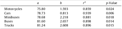
traffic flow. Based on these curves, we estimated the regression equation for a logarithmic model (log10) (Table 5).
The regression analyses were significant in all cases (p< 0.05) and explained nearly 90% of the continuous equivalent level. One of the most relevant results was that the sound pressure associated with the car flow becomes saturated at 600 veh/h, so increases in the car volume do not increase the level of traffic noise. In contrast, for other types of vehicles, monotonic growth was observed, which was likely due to the lower flows assessed (<200 veh/h), with in-creases in flows leading to inin-creases in noise, with the highest rates being related to buses and heavy trucks.
4. Conclusions
This report presented the development of a stochastic model for which performance on two-lane roads was better than that of well-recognized deterministic models, and this can be explained by the use of single noise recordings characteristic of the city of Bogotá. The model is promising, as it presents the possibility of an ap-proach that is more appropriate than deterministic models for addressing urban traffic conditions and, thus, traffic noise, which cannot be represented by macroscopic models. The stochastic model may include stochastic variables to emulate specific traffic characteristics, to try to improve predictions or to simulate specific conditions.
Additionally, the structure of the proposed stochastic model can be generalized to other conditions, though this requires traffic noise levels that are specific to the area under study. Furthermore, a simple deterministic model can be defined that resembles the TNM of the FHWA for this stochastic model. However, this model should be tested more widely under different of emissions and propagation conditions.
Regression analyses between noise levels of traffic origin and the abundance of vehicles show widely differing results, which stimulates the search for new methodological approaches, such as the one outlined here. The situation of the European models evaluated in this study is not very different to the regression anal-ysis in that it constitutes an extension of it, although the determin-istic models certainly achieve better performance in the simulation of urban traffic noise.
Appendix A. Supplementary material
Supplementary data associated with this article can be found, in the online version, at http://dx.doi.org/10.1016/j.apacoust.2012. 08.001.
References
[1] USEPA – US Environmental Protection Agency. Protective noise levels. Condensed version of EPA levels document, Washington, DC; 1978. [2] United Nations. World urbanization prospects: the 2003 revision. New York;
2004.
[3] Bolund P, Hunhammar S. Ecosystem services in urban areas. Ecol Econ 1999;29:293–301.
[4] COM, Propuesta de Directiva del Parlamento Europeo y del Consejo sobre evaluación y gestión del ruido ambiental, Informe final; 2000.
[5] EC-WGAEN – European Commission Working Group Assessment of Exposure to Noise. Good practice guide for strategic noise mapping and the production of associated data on noise exposure. Assessment of exposure to noise brussel. European Commission’s Working Group; 2006.
[6] Barrigón-Morillas JM, Gómez-Escobar V, Méndez-Sierra JA, Vílchez-Gómez R, Trujillo-Carmona J. An environmental noise study in the city of Cáceres. Spain. Appl Acoust 2002;63:1061–70.
[7] Alimohammadi I, Nassiri P, Behzad M, Hosseini MR. Reliability analysis of traffic noise estimation in highways of Tehran by Monte Carlo Simulation method. Iran J Environ Health Sci Eng 2005;2(4):229–36.
[8] Ingle ST, Pachpande BG, Wagh ND, Attarde SB. Noise exposure and hearing loss among the traffic policemen working at busy streets of Jalgaon urban centre. Transport Res Part D 2005;10:69–75.
[9] Ali SA, Tamura A. Road traffic noise levels, restrictions and annoyance in Greater Cairo. Egypt. Appl Acoust 2003;64:815–23.
[10] Li B, Tao S, Dawson RW. Evaluation and analysis of traffic noise from the main urban roads in Beijing. Appl Acoust 2002;63:1137–42.
[11] Calixto A, Diniz FB, Zannin PHT. The statistical modeling of road traffic noise in an urban setting. Cities 2003;20(1):23–9.
[12] Zuluaga CL, Correa MA, González AE. Desarrollo de un modelo matemático para la estimación de los niveles de ruido procedente del tráfico rodado en centros urbanos. In: VI Congreso Iberoamericano de Acústica, Buenos Aires; November 5 a 7, 2008.
[13] Ramírez A. Caracterización y modelación micro y macroscópica del ruido vehicular en la ciudad de Bogotá. PhD Thesis, Pontificia Universidad Javeriana, Bogotá; 2012.
[14] NRC – National Research Council. Models in environmental regulatory decision making. Committee on models in the regulatory decision process. Washington, DC: National Academies; 2007.
[15] FTA – Federal Transit Administration. Transit noise and vibration impact assessment, Washington, DC; 2006.
[16] Puigdomènech J, Jorge J, Mulet J. Acoustical impact of roads on medium-sized mediterranean coastal towns. Appl Acoust 1996;47:83–92.
[17] Bhaskar A, Chung E, Kuwahara M. Development and implementation of the area wide Dynamic Road traffic NoisE (DRONE) simulator. Transport Res Part D 2007;12:371–8.
[18] Tang UW, Wang ZS. Influences of urban forms on traffic-induced noise and air pollution: results from a modelling system. Environ Modell Softw 2007;22:1750–64.
[19] Trombetta PH, Queiroz D. Noise mapping at different stages of a freeway redevelopment project – a case study in Brazil. Appl Acoust 2011;72:479–86. [20] Murphy E, King EA. Scenario analysis and noise action planning: modelling the impact of mitigation measures on population exposure. Appl Acoust 2011;72:487–94.
[21] Seong JC, Park TH, Ko JH, Chang SI, Kim M, Holt JB, et al. Modeling of road traffic noise and estimated human exposure in Fulton County, Georgia, USA. Environ Int 2011;37:1336–41.
[22] Recuero M, Gil C, Grundman J, Sancho J. Prediction equations of outdoor acoustic noise in some towns of Madrid. In: Proceedings of inter-noise vol. 97; 1997, p. 843–46.
[23] Steele C. A critical review of some traffic noise prediction models. Appl Acoust 2001;62:271–87.
[24] Banerjee D, Chakraborty SK, Bhattacharyya S, Gangopadhyay A. Modeling of road traffic noise in the industrial town of Asansol, India. Transport Res D 2008;13:539–41.
[25] Arana M, Martínez de Vírgala A, Aleixandre A, San Martín ML, Vela A. Modelos de predicción del ruido de tráfico rodado. Comparación de diferentes standards europeos. Navarra: Univ. Púb.; 2000.
[26] Austroads, modelling, measuring and mitigating road traffic noise. Project No. TP1085, Sydney; 2005.
[27] FHWA – US Department of Transportation Federal Highway Administration. Traffic noise model. Version 2.5 look-up tables user’s guide, FHWA-HEP-05-008. DOT-VNTSC-FHWA-0406. Final Report; 2004.
[28] Janczur R, Walerian E, Czechowicz M. Influence of vehicle noise emission directivity on sound level distribution in a canyon street. Part I: Simulation program test. Appl Acoust 2006;67:643–58.
[29] Jraiw KS. A computer model to assess and predict road transport noise in built-up areas. Appl Acoust 1987;21:147–62.
[30] Pamanikabud P, Tansatcha M. Geographical information system for traffic noise analysis and forecasting with the appearance of barriers. Environ Modell Softw 2003;18:959–73.
[31] Can A, Leclercq L, Lelong J, Defrance J. Capturing urban traffic noise dynamics through relevant descriptors. Appl Acoust 2008;69(12):1270–80.
[32] Abo-Qudais SA, Alhiary A. Statistical models for traffic noise at signalized intersections. Build Environ 2007;42:2939–48.
[33] Cammarata G, Cavalieri S, Fichera A. A neural network architecture for noise prediction. Neural Networks 1995;8(6):963–73.
[34] Genaro N, Torija A, Ramos A, Requena I, Ruiz DP, Zamorano M. Modeling environmental noise using artificial neural networks. In: Ninth international conference on intelligent systems design and applications, Pisa; 2009. p. 215– 19.
[35] Can A, Leclercq L, Lelong J. Dynamic estimation of urban traffic noise: influence of traffic and noise source representations. Appl Acoust 2008;69(10):858–67.
Table 5
Regression analysis between the traffic flow (log) and the continuous equivalent level (a: intercept;b: slope;r2: coefficient of determination;p-value: regression signifi-cance level).
a b r2 p-Value
Motorcycles 75.80 1.593 0.859 0.024
Cars 78.73 0.813 0.939 0.006
Minibuses 78.68 2.218 0.881 0.018
Buses 81.60 2.657 0.898 0.014
Trucks 81.24 2.608 0.896 0.015
[36] De Coensel B, De Muer T, Yperman I, Botteldooren D. The influence of traffic flow dynamics on urban soundscapes. Appl Acoust 2005;66:175–94. [37] Pamanikabud P, Tansatcha M, Brown AL. Development of a highway noise
prediction model using an Leq20s measure of basic vehicular noise. J Sound Vib 2008;316:317–30.
[38] Duque MA, Ladino E. Modelación matemática del ruido producido por el tráfico en seis puntos ubicados en la ciudad de Pereira, Tesis Especialización en Vías y Transporte. Univ. Nal. Colombia, Manizales; 2007.
[39] STT – Secretaría de Tránsito y Transporte. Diagnóstico y caracterización de la contaminación auditiva producida por fuentes móviles en la ciudad de Bogotá y diseño de estrategias de mitigación de impactos negativos de la movilidad por emisiones sonoras. Fase II: Elaboración de modelos, monitoreo y toma de información, CONTRATO INAM Ltda., 170/05, Bogotá; 2006.
[40] Abbott PG, Nelson PM. Converting the UK traffic noise index LA10, 18h to EU noise indices for noise mapping. Project Report PR/SE/451/02. Crowthorne: TRL Ltd.; 2002.
[41] Kragh J, Plovsing B, Storeheier SÅ, Taraldsen G, Jonasson HG. Nordic environmental noise prediction methods, Nord2000. Summary Report, General nordic sound propagation model and applications in source-related
prediction methods. DELTA Acoustics & Vibration Report AV 1719/01. Lyngby, Denmark; 2002.
[42] Domínguez E, Dawson CW, Ramírez A, Abrahart RJ. The search for orthogonal hydrological modeling metrics: a case study of 20 monitoring stations in Colombia. J Hydroinformatics 2011;13(3):429–42.
[43] Dhingra SL, Gull I. Traffic flow theory historical research perspectives. In: Symposium on the Fundamental Diagram: 75 Years (Greenshields 75 Symposium), Woods Hole, MA; July 8–10, 2008. p. 19.
[44] Law CW, Lee CK, Lui ASW, Yeung MKL, Lam KC. Advancement of three-dimensional noise mapping in Hong Kong. Appl Acoust 2011;72:534–43. [45] Ko JH, Chang S, Lee BC. Noise impact assessment by utilizing noise map and
GIS: a case study in the city of Chungju, Republic of Korea. Appl Acoust 2011;72:544–50.
[46] González AE. Noise sources in the city: characterization and management trends. In: Siano D, editor. Noise control, reduction and cancellation solutions in engineering. In Tech, Croatia; 2012, p. 3–26.