Computational Intelligence and Big data Analytics Application in Bioinformatics pdf pdf

(1)

T E C H N O LO G Y 

_{FORENSIC AND MEDICAL BIOINFORMATICS}

Ch. Satyanarayana

Kunjam Nageswara Rao

Richard G. Bush

Computational

Intelligence

and Big Data

Analytics

(2)

SpringerBriefs in Applied Sciences

and Technology

Forensic and Medical Bioinformatics

Series editors

(3)

(4)

Ch. Satyanarayana

•

Kunjam Nageswara Rao

Richard G. Bush

Computational Intelligence

and Big Data Analytics

Applications in Bioinformatics

(5)

Department of Computer Science

ISSN 2191-530X ISSN 2191-5318 (electronic)

SpringerBriefs in Applied Sciences and Technology

ISSN 2196-8845 ISSN 2196-8853 (electronic)

SpringerBriefs in Forensic and Medical Bioinformatics

ISBN 978-981-13-0543-6 ISBN 978-981-13-0544-3 (eBook) https://doi.org/10.1007/978-981-13-0544-3

Library of Congress Control Number: 2018949342 ©_{The Author(s) 2019}

This work is subject to copyright. All rights are reserved by the Publisher, whether the whole or part of the material is concerned, speciﬁcally the rights of translation, reprinting, reuse of illustrations, recitation, broadcasting, reproduction on microﬁlms or in any other physical way, and transmission or information storage and retrieval, electronic adaptation, computer software, or by similar or dissimilar methodology now known or hereafter developed.

The use of general descriptive names, registered names, trademarks, service marks, etc. in this publication does not imply, even in the absence of a speciﬁc statement, that such names are exempt from the relevant protective laws and regulations and therefore free for general use.

The publisher, the authors and the editors are safe to assume that the advice and information in this book are believed to be true and accurate at the date of publication. Neither the publisher nor the authors or the editors give a warranty, express or implied, with respect to the material contained herein or for any errors or omissions that may have been made. The publisher remains neutral with regard to jurisdictional claims in published maps and institutional afﬁliations.

(6)

Chapter 1 A Novel Level-Based DNA Security

Algorithm Using DNA Codons

Bharathi Devi Patnala and R. Kiran Kumar

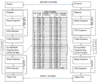
Abstract Providing security to the information has become more prominent due to the extensive usage of the Internet. The risk of storing the data has become a serious problem as the numbers of threats have increased with the growth of the emerging technologies. To overcome this problem, it is essential to encrypt the information before sending it to the communication channels to display it as a code. The silicon computers may be replaced by DNA computers in the near future as it is believed that DNA computers can store the entire information of the world in few grams of DNA. Hence, researchers attributed much of their work in DNA computing. One of the new and emerging fields of DNA computing is DNA cryptography which plays a vital role. In this paper, we proposed a DNA-based security algorithm using DNA Codons. This algorithm uses substitution method in which the substitution is done based on the Lookup table which contains the DNA Codons and their corresponding equivalent alphabet values. This table is randomly arranged, and it can be transmitted to the receiver through the secure media. The central idea of DNA molecules is to store information for long term. The test results proved that it is more powerful and reliable than the existing algorithms.

Keywords Encryption

_·

Decryption

_·

Cryptography

_·

DNA Codons

_·

DNA cryptography

_·

DNA strand

1.1 Introduction

DNA computing is introduced by Leonard Adleman, University of Southern Califor-nia, in the year 1994. He explained how to solve the mathematical complex problem Hamiltonian path using DNA computing in lesser time [1]. He envisioned the use of DNA computing for any type of computational problems that require a massive amount of parallel computing. Later, Gehani et al. introduced a concept of DNA-based cryptography which will be used in the coming era [2]. DNA cryptography is one of the rapidly emerging technologies that works on concepts of DNA com-puting. DNA is used to store and transmit the data. DNA computing in the fields of

Ch. Satyanarayana et al.,Computational Intelligence and Big Data Analytics,

SpringerBriefs in Forensic and Medical Bioinformatics, https://doi.org/10.1007/978-981-13-0544-3_1

(11)

Table 1.1 DNA table _Bases _{Gray coding}

A 00

G 01

C 10

T 11

cryptography and steganography has been identified as a latest technology that may create a new hope for unbreakable algorithms [3].

The study of DNA cryptography is based on DNA and one-time pads, a type of encryption that, if used correctly, is virtually impossible to crack [4]. Many traditional algorithms like DES, IDEA, and AES are used for data encryption and decryption to achieve a very high level of security. However, a high quantum of investigation is deployed to find the key values that are required by buoyant factorization of large prime numbers and the elliptic cryptography curve problem [5]. Deoxyribonucleic acid (DNA) contains all genetic instructions used for development and functioning of each living organisms and few viruses. DNA strand is a long polymer of millions of linked nucleotides. It contains four nucleotide bases named as Adanine (A), Cytosine (C), Glynase (G), and Thymine (T). To store this information, two bits are enough for each nucleotide. The entire information will be stored in the form of nucleotides. These nucleotides are paired with each other in double DNA strand. The Adanine is paired with Thymine, i.e., A with T, and the Cytosine is paired with Glynase, i.e., C with G.

1.2 Related Work

(12)

Table 1.2 Structured DNA Codons [9]

[10]. This gives rise to ambiguity like Phenylalanine amino acid mapped on TTT and TTC. To overcome this, we prepared a Lookup table (Table1.3) for each Codon. A Codon is a sequence of three adjacent nucleotides constituting the genetic code that specifies the insertion of an amino acid in a specific structural position in a polypeptide chain during the synthesis of proteins.

1.3 Proposed Algorithm

(13)

Table 1.3 Lookup table

• Each letter in the plaintext is converted into its ASCII code. • Each letter in the plaintext is converted into its ASCII code. • The binary code will be split into two bits each.

• Each two bits of the binary code will be replaced by its equivalent DNA nucleotides from Table1.1.

Round 2:

• From the derived DNA strand, three nucleotides will be combined to form a Codon. • Each Codon will be replaced by its equivalent from the Lookup Table1.3.

Round 3:

(14)

Fig. 1.1 DNA structure [6]

• Again, the ASCII codes will be converted into its equivalent binary code. • Again, the binary code will be split into two bits each.

• Each two bits of the binary code will be replaced by its equivalent DNA nucleotide from Table1.1. The DNA strand so generated will be the final ciphertext (Fig.1.1).

1.3.2 Decryption Algorithm

The process of reversing the steps from last to first in all rounds continuously will create decryption algorithm.

The algorithm uses the following three levels to complete the encryption. It is briefly described in the Fig.1.2.

1.4 Algorithm Implementation

1.4.1 Encryption

(15)

Fig. 1.2 DNA-based cryptography method using DNA Codons

Round 1:

Round 2:

The DNA strand from the above round is

CACACGCCCTATCGGCCTAGCGCC

(16)

Round 3:

The ciphertext is CCGGCGTGCCCGCAGCCGCGCCCCCTCAATAC

1.4.2 Decryption

The process is done from last to first round to get the plaintext.

In this algorithm three letters forming a Codon and hence all characters the plain-text contains, divisible by 3 is only encrypted into cipherplain-text. If the characters that are in the plaintext leaves a remainder, when divided by three can be converted with the help of padding to display as ciphertext.

(17)

1.5 Experimental Results

1.5.1 Encryption Process

(18)

1.5.3 Padding of Bits

The encryption and decryption processes are the same as above in all the cases.

1.5.3.1 Encryption Process

If the number of characters of a plaintext is not divisible by 3, then

(19)

(20)

1.5.3.2 Decryption Process

If the number of characters of a plaintext is not divisible by 3, then

(21)

1.6 Result Analysis

Let the sender send the ciphertext in the form of DNA to the receiver end. Suppose the length of plaintext is “m”. Three cases can be discussed here. Case 1: The plaintext (m) is divisible by 3:

When the plaintext (m) is converted into DNA, the length is increased tom* 4, saym1. In the second level, the DNA nucleotides are divided into Codons. So, the length ism1/3, say m2. In the third level, the Codons can be replaced with their equivalent replaceable character from the Lookup table (Table1.3). Again these can be converted into DNA which is our ciphertext of lengthm2 * 4, say m3.

Case 2: The number of characters of plaintext (m) is not divisible by 3, and it leaves the remainder 1:

Then we add additional 2 nucleotides to make a Codon. So,m1m* 4 + 2 and

m2,m3 is calculated similarly.

Case 3: The number of characters of plaintext is not divisible by 3 and leaves the remainder 2:

We add additional 1 nucleotide to make a Codon. Here,m1m* 4 + 1 andm2,

m3 is calculated similarly.

Based uponm1,m2, andm3, we calculate the length of ciphertext in each level. The final length of cipher ism3. Hence, the time complexity of the encryption process is

O(m), and the same process is done in the receiver end also so that the time complexity of decryption process isO(m).

The simulations are performed by using .net programming on Windows 7 system. The hardware configuration of the system used is Core i3 processor/4 GB RAM. The following table shows the performance of the proposed algorithm with different sets of plaintext varying in length. The observations from the simulation have been plotted in Fig.1.3and shown in Table1.4.

From the above table and graph, it can be observed that as the length of plaintext increased, the encryption and decryption times have also increased.

(22)

Table 1.4 Length–time analysis

S. No. Length of plaintext (in

terms of bytes)

Encryption time (ms) Decryption time (ms)

1 10 0.0043409 0.0001647

2 100 0.0123234 0.0006070

3 1000 0.1116644 0.0020742

4 10,000 14.0743528 0.0333596

1.7 Conclusions

Security plays a vital role in transferring the data over different networks, and several algorithms were designed to enhance the security at various levels of network. In the absence of security, we cannot assure the users to route the data freely. In traditional cryptography, as the earlier algorithms could not provide security as desired, we have in full confidence, drawn the present algorithm based on DNA cryptography, that is developed using DNA Codons. It assures a perfect security for plaintext in modern technology as each Codon can be replaced in 64 ways from the Lookup table randomly.

References

1. Adleman LM (1994) Molecular computation of solution to combinatorial problems. Science, New Series, 266(5187):1021–1024

2. Gehani A, Thomas L, Reif J (2004) DNA-based cryptography-in aspects of molecular com-puting. Springer, Berlin, Heiderlberg, pp 167–188

3. Nixon D (2003) DNA and DNA computing in security practices-is the future in our genes? Global information assurance certification paper, Ver.1.3

4. Popovici C (2010) Aspects of DNA cryptography. Ann Univ Craiova, Math Comput Sci Ser 37(3):147–151

5. Babu ES, Nagaraju C, Krishna Prasad MHM (2015) Light-weighted DNA based hybrid cryp-tographic mechanism against chosen cipher text attacks. Int J Inf Process 9(2):57–75 6. http://www.chemguide.co.uk/organicprops/aminoacids/doublehelix.gif

7. Yamuna M, Bagmar N (2013) Text Encryption using DNA steganography. Int J Emerg Trends Technol Comput Sci (IJETTCS) 2(2)

8. Reddy RPK, Nagaraju C, Subramanyam N (2014) Text Encryption through level based privacy using DNA Steganography. Int J Emerg Trends Technol Comput Sci (IJETTCS) 3(3):168–172 9. http://www.chemguide.co.uk/organicprops/aminoacids/dnacode.gif

(23)

Cognitive State Classifiers for Identifying

Brain Activities

B. Rakesh, T. Kavitha, K. Lalitha, K. Thejaswi and Naresh Babu Muppalaneni

Abstract The human brain activities’ research is one of the emerging research areas, and it is increasing rapidly from the last decade. This rapid growth is mainly due to the functional magnetic resonance imaging (fMRI). The fMRI is rigorously using in testing the theory about activation location of various brain activities and produces three-dimensional images related to the human subjects. In this paper, we studied about different classification learning methods to the problem of classifying the cog-nitive state of human subject based on fMRI data observed over single-time interval. The main goal of these approaches is to reveal the information represented in vox-els of the neurons and classify them in relevant classes. The trained classifiers to differentiate cognitive state like (1) Does the subject watching is a word describing buildings, people, food (2) Does the subject is reading an ambiguous or non ambigu-ous sentence and (3) Does the human subject is a sentence or a picture etc. This paper summarizes the different classifiers obtained for above case studies to train classifiers for human brain activities.

Keywords Classification

·

fMRI

·

Support vector machines

·

Naïve Bayes

2.1 Introduction

The main issue in cognitive neuroscience is to find the mental faculties of different tasks, and how these mental states are converted into neural activity of brain [1]. The brain mapping is defined as association of cognitive states that are perceptual with patterns of brain activity. fMRI or ECOG is used to measure persistently with multiunit arrays of brain activities [1]. Non-persistently, EEG and NIRS (Near Infrared Spectroscopy) are used for measuring the brain functions. These devel-opment machines are used in conjunction with modern machine learning and pattern recognition techniques for decoding brain information [1]. For both clinical and research purposes, this fMRI technique is most reputed scheme for accessing the brain topography. To find the brain regions, the conventional univariate analysis of fMRI data is used, the multivariate analysis methods decode the stimuli, and cognitive

Ch. Satyanarayana et al.,Computational Intelligence and Big Data Analytics, SpringerBriefs in Forensic and Medical Bioinformatics,

https://doi.org/10.1007/978-981-13-0544-3_2

(24)

EEG-fMRI

Fig. 2.1 Architecture of fMRI-EEG analysis

states the human from the brain fMRI activation patterns [1]. The multivariate anal-ysis methods use various classifiers such as SVM, naïve Bayes which are used to decode the mental processes of neural activity patterns of human brain. Present-day statistical learning methods are used as powerful tools for analyzing functional brain imaging data.

After the data collection to detect cognitive states, train them with machine learn-ing classifier methods for decodlearn-ing its states of human activities [2]. If the data is sparse, noisy, and high dimensional, the machine learning classifiers are applied on the above-specified data.

Combined EEG and fMRI data are used to classify the brain activities by using SVM classification algorithm. For data acquisition, EEG equipment, which compat-ible with 128 channel MR and 3 T Philips MRI scanners, is used [3]. These analyses give EEG-fMRI data which has better classification accuracy compared with fMRI data alone.

2.2 Materials and Methods

2.2.1 fMRI-EEG Analysis

(25)

to analyze fMRI data [1]. These models could not describe the stimulus but they recovered the state as hidden state by HMM. The other way to analyze fMRI data is unsupervised learning.

2.2.2 Classification Algorithms

2.2.2.1 Naïve Bayes Classifier

This classifier is one of the widely used classification algorithms. This is one of the statistical and statistical methods for classification [1]. It predicts the conditional probability of attributes. In this algorithm, the effect of one attributeXiis independent of other attributes. This is called as conditional independence, and this algorithm is based on Bayes’ theorem [1]. To compute the probability of attributesX1,X2,X3,X4, …,Xnof a classCthis Bayes’ theorem is used and it can perform classifications. The posterior probability by Bayes’ theorem can be formulated as:

P likelihood×prior

evidence

2.2.2.2 Support Vector Machine

Support vector machines are commonly used for learning tasks, regression, and data classification. The data classifications are divided into two sets, namely training and testing sets. Training set contains the class labels called target value and several observed variables [1–3]. The main goal of this support vector machine is used to find the target values of the test data.

Let us consider the training attributesXi, wherei{1, 2, …n} and training labels z{I,−1}. The test data labels can be predicted by the solution of the below given optimization problem

Where 1 _i_≥_0,_φ_{is hyperplane for separating training data,}_C_{is the penalty}

(26)

Table 2.1 Classifiers error rates

40 Yes 0.183 0.112 0.190

40 No 0.342 0.341 0.381

Categories of semantics

32 Yes 0.081 NA 0.141

32 No 0.102 NA 0.251

Ambiguity of syntactic

10 Yes 0.251 0.278 0.341

10 No 0.412 0.382 0.432

2.2.2.3 K-Nearest Neighbor Classifier

Thek-nearest neighbor classifier is the simplest type of classifier for pattern recog-nition. Based upon its closest training examples, it classifies the test examples and test example label is calculated by the closest training examples labels [6]. In this classifier, Euclidean distance is used a distance metric.

Let us consider, the Euclidian can be represented asE, and then

E2(b,x)(b−x)(b−x)′

wherexandbare row vectors withmfeatures.

2.2.2.4 Gaussian Naïve Bayes Classifier

For fMRI observations, the GNN classifier uses the training data to estimate the probability distribution based on the humans cognitive states [7]. It classifies new exampleY′ _{_Y state cifor given fMRI observations.

The probability can be estimated by using the Bayes’ rule

M(ci|Y′)

(27)

0 0.1 0.2 0.3 0.4 0.5

Yes No Yes No Yes No

40 40 32 32 10 10

Sentence vs Picture Categories of semantics Ambiguity of syntactic

GNB

SVM

9NN

Fig. 2.2 Comparative analysis of GNB, SVM, kNN

2.3 Results

The results shown in the table give better performing variants of GNB, and we can observe the table GNB and SVM classifiers outperformed kNN. The performance generally improves the increasing values ofk(Fig.2.2).

2.4 Conclusion

In this paper, we represented results from three different classifiers of fMRI studies representing the feasibility of training classifiers to distinguish a variety of cogni-tive states. The comparison indicates that linear support vector machine (SVM) and Gaussian naive Bayes (GNB) classifiers outperform K-nearest neighbor [2]. The accuracy of SVMs increases rapidly than the accurateness of GNB as the dimension of data is decreased through feature selection. We found that the feature selection methods always enhance the classification error in all three studies. For the noisy, high-dimensional, sparse data, feature selection is a significant aspect in the design of classifiers [1]. The results showed that it is possible to use linear support vector machine classification to accurately predict a human observer’s ability to recognize a natural scene photograph [8]. Furthermore, classification provides a simply inter-pretable measure of the significance of the informative brain activations: the quantity of accurate predictions.

References

1. Ahmad RF, Malik AS, Kamel N, Reza F (2015) Object categories specific brain activity classi-fication with simultaneous EEG-fMRI. IEEE, Piscataway

(28)

3. Tom M, Mitchell et al (2008) Predicting human brain activity associated with the meanings of nouns. Science 320:1191.https://doi.org/10.1126/science.1152876

4. Rieger et al (2008) Predicting the recognition of natural scenes from single trial MEG recordings of brain activity.

5. Taghizadeh-Sarabi M, Daliri MR, Niksirat KS (2014) Decoding objects of basic categories from electroencephalographic signals using wavelet transform and support vector machines. Brain topography, pp 1–14

6. Miyapuram KP, Schultz W, Tobler PN (2013) Predicting the imagined contents using brain acti-vation. In: Fourth national conference on computer vision pattern recognition image processing and graphics (NCVPRIPG) 2013, pp 1–3

(29)

Multiple DG Placement and Sizing

in Radial Distribution System Using

Genetic Algorithm and Particle Swarm

Optimization

M. S. Sujatha, V. Roja and T. Nageswara Prasad

Abstract The present day power distribution network is facing a challenging role to cope up for continuous increasing of load demand. This increasing load demand causes voltage reduction and losses in the distribution network. In current years, the utilization of DG technologies has extremely inflated worldwide as a result of their potential benefits. Optimal sizing and location of DG units near to the load cen-ters provide an effective solution for reducing the system losses and improvement in voltage and reliability. In this paper, the effectiveness of genetic algorithm (GA) and particle swarm optimization (PSO) for optimal placement and sizing of DG in the radial distribution system is discussed. The main advantage of these methods is computational robustness. They provide an optimal solution in terms of improvement of voltage profile, reliability, and also minimization of the losses. They provide the best resolution in terms of improvement of voltage profile, reliability, and also mini-mization of the losses. The anticipated algorithms are tested on IEEE 33- and 69-bus radial distribution systems using multi-objective function, and results are compared.

Keywords Distributed generation

·

Genetic algorithm

·

Particle swarm

optimization

·

Multi objective function

·

Optimum location

·

Loss minimization

·

Voltage profile improvement

3.1 Introduction

The operation of the power system network is too complicated, especially in urban areas, due to the ever-increasing power demand and load density. In the recent past, hydro-, atomic, thermal, and fossil fuel-based generation power plants were in use to meet the energy demands. Centralized control system is used for the operation of such generation systems. Long-distance transmission and distribution systems are used for delivering power to meet the demands of consumers. Due to the depletion of con-ventional resources and increased transmission and distribution costs, concon-ventional power plants are on the decline [1].

Ch. Satyanarayana et al.,Computational Intelligence and Big Data Analytics, SpringerBriefs in Forensic and Medical Bioinformatics,

https://doi.org/10.1007/978-981-13-0544-3_3

(30)

Distributed generation (DG) is an alternative solution to overcome various power systems problems such as generation, transmission and distribution costs, power loss, voltage regulation [2]. Distributed generation is generation of electric power in small-scale on-site or near to the load center. Several studies revealed that there are potential benefits from DG [3]. Though the DG has several benefits, the most difficulty in placement of DG is that the choice of best location, size, and range of DG units. If the DG units are not properly set and sized, it results in volt-age fluctuations, upper system losses, and raise in operational prices. To reduce the losses, the best size and location are very important [4–8]. The selection of objective function is one of the factors that influence the system losses [9–11]. In addition to loss reduction, reliability is also an important parameter in DG placement [12,13]. In recent years, many researchers have projected analytical approaches based on sta-bility and sensitivity indices to locate the DG in radial distribution systems [14–18]. Viral and Khatod [17] projected a logical method for sitting and sizing of DGs. With this method, convergence can be obtained in a few iterations but is not suitable for unbalanced systems. By considering multiple DGs and different load models, loss reduction and voltage variations are discussed in [19–23]. The authors of [24] con-sidered firefly algorithm for finding DG placement and size to scale back the losses, enhancement of voltage profile, and decrease of generation price. But the drawback of this method is slow rate of convergence. Bat algorithm and multi-objective shuf-fled bat algorithms are used in [25] and [26], respectively, for optimal placement and sizing of DG in order to meet the multi-objective function. Mishra [27] proposed DG models for optimal location of DG for decrease of loss. Optimization using genetic algorithm is proposed in [28]. The particle swarm optimization is presented in [29] for loss reduction. The authors of [30] discussed the minimization of losses by optimal DG allocation in the distribution system.

This paper is intended to rise above all drawbacks by considering multi-objective function for most favorable sizing and placing of multi-DG with genetic algorithm and particle swarm optimization techniques, and the effectiveness of these algorithms is tested on different test systems.

3.2 DG Technologies

(31)

3.2.1 Number of DG Units

The placing of DGs may be either single or multiple DG units. Here, multiple DG approach is considered consisting of three DGs in the test system of radial distribution system for loss reduction [22].

3.2.2 Types of DG Units

Based on power-delivering capacity, the DGs are divided into four types [22]. Type-1: DG injecting active power at unity PF. Ex. Photovoltaic; Type-2: DG injecting reactive power at zero PF. Ex. gas turbines; Type-3: DG injecting active power but consuming reactive power at PF ranging between 0 and 1. Ex. wind farms; Type-4: DG injecting both active and reactive powers at PF ranging between 0 and 1. Ex. Synchronous generators.

3.3 Mathematical Analysis

3.3.1 Types of Loads

Loads may be of different types, viz., domestic loads, commercial loads, industrial loads, and municipal loads.

3.3.2 Load Models

In the realistic system, loads do not seem to be only industrial, commercial, and residential; but it is depending on nature of the area being supplied [21]. Practical voltage-depended load models are considered in [8]. The recently developed numer-ical equations for different load models in the system are specified by Eqs. (1) and (2).

QD0iat Bus I are demand operating points of active and reactive powers,V0is voltage

(32)

Table 3.1 Load models of exponent values

Type of load Exponents Load type Exponents

Constant load α00 β00 Residential load αr 0.92 βr

4.04

Industrial load αi 0.18 βi6 Commercial load αc 1.51 βc

3.4

power exponents for industrial, commercial, residential, and constant load models with subscriptions i, c, r, and 0, respectively.

Table3.1indicates exponent values of the different load models. p1, q1, r1, s1are

the weight coefficients of active power andp2, q2, r2, s2are the weight coefficients of

reactive power respectively. The exponent values of coefficients for different loads and types are specified as below:

Type-1: Constant load:p11,q10,r10,s10,p21,q20.r20,s20.

Type-2: Industrial load:p10,q11,r10,s10,p20,q21.r20,s20.

Type-3: Residential load:p10,q10,r11,s10,p20,q20.r21,s2

0.

Type-4: Commercial load:p10,q10,r10,s11,p20,q2 0.r20,s2

1.

Load type-5: Mixed or practical load:p1ta1,q1ta2,r1= ta3,s1ta4 andP2=

trl,q2tr2,r2tr3,s2tr4. Also for the practical mixed load models, ta1 + ta2 +

ta3 + ta41 and tr 1 + tr2 + tr3 + tr41.

3.3.3 Multi-objective Function (MOF)

The multi-objective function given in (3) can be used for most favorable position and sizing of multi-DG using GA and PSO techniques.

M O F C1P L I+C2Q L I+C3V D I+C4R I+C5S F I (3)

where PLI,QLI,VDI,RI, andSFIare active power loss, reactive power loss, volt-age deviation, reliability, and sensitivity or shift factor of the system, explained in Eqs. (8)–(12), respectively.C1,C2,C3,C4,andC5are the weight factors of the indices

of the system. The active and reactive losses are given in the following Eqs. (4) and (5).

• Real power loss (PL)

P L

N

K1

(33)

• Reactive power loss (QL)

whereIkis branch current,Rkresistance;Xkreactance ofkth line [27],IKPpeak load

branch current,λkfailure rate forkth branch or line,Vratedsystem rated voltage,α

load factor, anddrepair duration.

• The reliability of the system is given as [12]

R1−

_{E N S}

P D

(7)

whereRis reliability andPDtotal power demand.

3.3.4 Evaluation of Performance Indices Can Be Given

by the Following Equations

where N is total number of buses, Vreff reference voltage, andVDGj DG system

voltage.

The equation of SFI by fitting of DG of suitable size can be expressed as [13]

S F I maxx−1

(34)

R I E N SDG

E N SN O−DG

(12)

whereENSDGis ENS by DG andENSNo−DGis ENS by without DG condition.

3.4 Proposed Methods

In this work, GA and PSO are the evolutionary techniques used for the planning of DGs.

3.4.1 Genetic Algorithm (GA)

It is one of the evolutionary algorithm techniques [10]. It is a robust optimization technique based on natural selection. In case of DG placement, fitness function can be loss minimization, voltage profile improvement, and cost reduction.

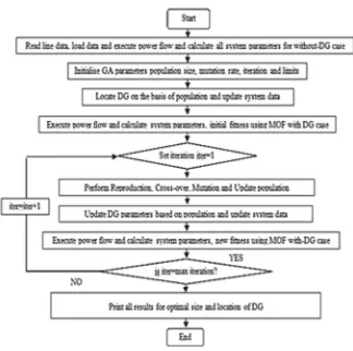
Figure3.1shows the flow sheet to seek out optimum sitting and size of DGs using GA in different test systems, where PDG, QDG, and LDG represent real and reactive powers and position of DG and are considered in the form of population.

3.4.2 Particle Swarm Optimization (PSO)

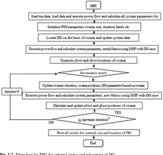
PSO is a population-based calculation and was presented by Dr. Kennedy and Dr. Eberhart in 1995. It is a biologically inspired algorithm [15]. It is a novel intelli-gence search algorithm [9] that provides good solution to the nonlinear complex optimization problem. Figure3.2demonstrates the procedure flowchart to discover ideal sitting and estimating of DGs in the different test frameworks utilizing PSO.

3.5 Results and Discussions

Results of best placing and size of multi-DG with MOF using GA and PSO in a particular type of system are presented in the following sections. MATLAB (2011a) is used to validate the proposed methodologies.

3.5.1 33-Bus Radial Distribution System

(35)

Fig. 3.1 Flowchart for GA for optimal sizing and placement of DG

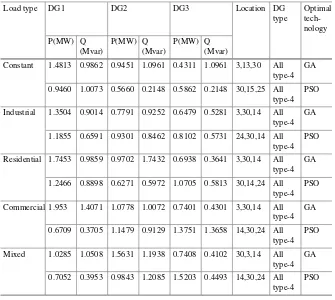
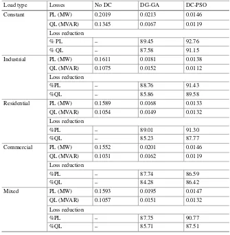
Table3.4shows that all type-4 DGs are suitable and are ideally introduced in 33-bus radial distribution system by utilizing GA and PSO techniques with various load models.

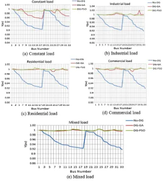
The active and reactive power loss reductions of 33-bus multi-DG structure are 89.45 and 87.58% for GA and 92.76 and 91.15% for PSO, respectively, and they are shown in Table3.6. Voltage profiles of 33-bus radial distribution system for various load models are shown in Fig.3.5. By observing this, the voltage profiles are better with DG than without DG and are farther improved with DG-PSO compared with DG-GA and without DG.

(36)

Fig. 3.2 Flowchart for PSO for optimal sizing and placement of DG

(37)

Table 3.2 ENS and reliability of 33-bus radial distribution system with multi-DG using GA and PSO

Load type Parameters No DG DG-GA DG-PSO

Constant ENS (MW) 0.1243 0.0103 0.0102

Reliability 0.9658 0.9970 0.9972

Industrial ENS (MW) 0.1038 0.0102 0.0038

Reliability 0.9715 0.9991 0.9986

Residential ENS (MW) 0.1068 0.0178 0.0035

Reliability 0.9650 0.9945 0.9987

Commercial ENS (MW) 0.1068 0.0091 0.0048

Reliability 0.9691 0.9972 0.9983

Mixed ENS (MW) 0.1055 0.0102 0.0032

Reliability 0.9705 0.9995 0.9991

Fig. 3.4 Active and reactive power losses with multi-DG and different load models of 33-bus radial system

3.5.2 69-Bus Radial Distribution System

(38)

Table 3.3 MOFand indices for 33-bus radial distribution system with multi-DG and different loads

Load type Fitness (MOF)

PLI QLI VDI Rl SFI Optimal

technology

Constant 0.1861 0.1051 0.1215 0.0125 0.0817 1.0549 GA

0.1635 0.0765 0.0905 0.0115 0.0812 1.0067 PSO

Industrial 0.1995 0.1190 0.1449 0.0115 0.0958 1.0411 GA

0.1718 0.0887 0.1106 0.0071 0.0385 1.0525 PSO

Residential 0.1989 0.1109 0.1359 0.0123 0.0172 1.0021 GA

0.1755 0.0971 0.1215 0.0056 0.0349 1.0322 PSO

Commercial 0.2039 0.1280 0.1551 0.0121 0.0875 1.0301 GA

0.1951 0.1210 0.1603 0.0063 0.0137 1.0210 PSO

Mixed 0.1978 0.1196 0.1435 0.0118 0.069 1.0311 GA

0.1736 0.0949 0.1155 0.0055 0.0306 1.0321 PSO

Table 3.4 Size and location of multiple DG in 33-bus radial distribution system

Load type DG1 DG2 DG3 Location DG

type

Constant 1.4813 0.9862 0.9451 1.0961 0.4311 1.0961 3,13,30 All

type-4 GA

0.9460 1.0073 0.5660 0.2148 0.5862 0.2148 30,15,25 All type-4

PSO

Industrial 1.3504 0.9014 0.7791 0.9252 0.6479 0.5281 3,30,14 All type-4

GA

1.1855 0.6591 0.9301 0.8462 0.8102 0.5731 24,30,14 All type-4

PSO

Residential 1.7453 0.9859 0.9702 1.7432 0.6938 0.3641 3,30,14 All type-4

GA

1.2466 0.8898 0.6271 0.5972 1.0705 0.5813 30,14,24 All type-4

PSO

Commercial 1.953 1.4071 1.0778 1.0072 0.7401 0.4301 3,30,14 All type-4

GA

0.6709 0.3705 1.1479 0.9129 1.3751 1.3658 14,30,24 All type-4

PSO

Mixed 1.0285 1.0508 1.5631 1.1938 0.7408 0.4102 30,3,14 All

type-4 GA

0.7052 0.3953 0.9843 1.2085 1.5203 0.4493 14,30,24 All type-4

(39)

Table 3.5 Active and reactive power losses of 33-bus radial distribution system with and without DG

Load type Losses No DC DG-GA DC-PSO

Constant PL (MW) 0.2019 0.0213 0.0146

QL (MVAR) 0.1345 0.0167 0.0119

Loss reduction

% PL – 89.45 92.76

% QL – 87.58 91.15

Industrial PL (MW) 0.1611 0.0181 0.0138

QL (MVAR) 0.1075 0.0152 0.0112

Loss reduction

%PL – 88.76 91.43

%QL – 85.86 89.58

Residential PL (MW) 0.1589 0.0168 0.0133

QL (MVAR) 0.1054 0.0149 0.0132

Loss reduction

%PL – 89.01 91.30

%QL – 85.23 87.77

Commercial PL (MW) 0.1552 0.0201 0.0146

QL (MVAR) 0.1031 0.0162 0.0119

Loss reduction

%PL – 87.74 86.59

%QL – 84.28 86.42

Mixed PL (MW) 0.1593 0.0195 0.0147

QL (MVAR) 0.1057 0.0151 0.0132

Loss reduction

%PL – 87.75 90.77

%QL – 85.71 87.51

Table 3.6 MOF and indices for 69-bus radial distribution system with multi-DG

Load type Fitness (MOF)

PLI QLI VDI RI SFI Optimal

technol-ogy

Mixed load

0.1612 0.0689 0.1168 0.0148 0.0015 1.0478 GA

(40)

Fig. 3.5 Voltage profiles of 33-bus radial system for different load models

(41)

Fig. 3.6 Energy not supplied and reliability of 33-bus radial distribution system

Fig. 3.7 A 69-bus radial distribution system

Table 3.7 Size and location for 69-bus radial distribution system with multi-DG

Load type

DG1 DG2 DG3 Location DG

type

Optimal tech-nology P(MW) Q(Mvar) P(MW) Q(Mvar) P(MW) Q(Mvar)

Mixed load

2.3030 2.4463 1.2769 0.8510 1.6290 1.2199 4,11,61 All

type-4 GA

3.3861 2.6942 0.7239 0.5564 1.7114 1.0616 4,12,61 All

(42)

Table 3.8 Active and reactive power losses of 69-bus radial distribution system with and without DG

Load type Losses No DG DG-GA DG-PSO

Mixed load PL (MW) QL 0.1703 0.0116 0.0085

(MVAR) 0.0788 0.0093 0.0083

Loss reduction

% PL – 93.18 95.00

% QL – 88.19 89.46

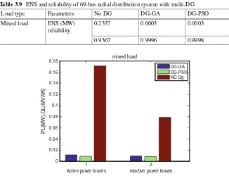
Table 3.9 ENS and reliability of 69-bus radial distribution system with multi-DG

Load type Parameters No DG DG-GA DG-PSO

Mixed load ENS (MW)

Active power losses reactive power losses

PL(MW),QL(MVAR)

mixed load

DG-GA DG-PSO NO Dg

Fig. 3.8 Active and reactive power losses of 69-bus radial distribution system

3.6 Conclusions

(43)

Fig. 3.9 Voltage profiles of 69-bus radial distribution system

References

1. Bohre AK, Agnihotri G (2016) Optimal sizing and sitting of DG with load models using soft computing techniques in practical distribution system. IET Gener Transm Distrib pp. 1–16 2. Ackermann T, Andersson G, Soder L (2001) Distributed generation: a definition. Electr Power

Syst Res 57:195–204

3. Chidareja P (2004) An approach to quantify technical benefits of distributed generation. IEEE Trans Energy 19(4):764–773

4. Viral R, Khatod DK (2012) optimal planning of DG systems in distribution system: a review. Int J Renew Sustain Energy Rev 16:5146–5165

5. Kalambe S, Agnihotri G (2014) Loss minimization techniques used in DN bibliographic survey. Int J Renew Sustain Energy Rev 29:184–200

6. Georgilakis Pavlos S, Hatziargyriou Nikos D (2013) Optimal distributed generation placement in power distribution networks: models, methods, and future research. IEEE Trans Power Syst 28(3):3420–3428

7. Ghosh S, Ghosh S (2010) Optimal sizing and placement of DG in a network system. Electr Power Energy Syst 32:849–856

8. Ghosh N, Sharma S, Bhattacharjee S (2012) A load flow based approach for optimal allocation of distributed generation units in the distributed network for voltage improvement and loss minimization. Int J Comput Appl 50(15):0975–8887

9. Singh D, Verma KS (2009) Multi objective optimization for DG planning with load models. IEEE Trans Power Syst 24(1):427–436

10. Ochoa LF, Padilha-Feltrin A, Harrison GP (2006) Evaluating DG impacts with a multi objective index. IEEE Trans Power Deliv 21(3):1452–1458

11. Pushpanjalli M, Sujatha MS (2015) A Navel multi objective under frequency load shedding in a micro grid using genetic algorithem. Int J Adv Res Electr Electron Instrum Eng 4(6) ISSN:2278–8875

(44)

13. Chowdhury AA, Agarwal SK, Koval DO (2003) Reliability modeling of distributed gen-eration in conventional distribution systems planning and analysis. IEEE Trans Ind Appl 39(5):1493–1498

14. Samui A, Singh S, Ghose T et al (2012) A direct approach to optimal feeder routing for radial distribution system. IEEE Trans Power Deliv 27(1):253–260

15. Acharya N, Mahat P, Mithulananthan N (2006) An analytical approach for DG allocation in primary distribution network. Int J Electric Power Energy Syst 28(10):669–678

16. Gopiya Naik SN, Khatod DK, Sharma MP (2015) Analytical approach for optimal siting and sizing of distributed generation in radial distribution networks. IET Gener Transm Distrib 9(3):209–220

17. Viral R, Khatod DK (2015) An analytical approach for sizing and siting of DGs in balanced radial distribution networks for loss minimization. Electric Power Energy Syst 67:191–201 18. Nahman JM, Dragoslav MP (2008) Optimal planning of radial distribution networks by

simu-lated annealing technique. IEEE Trans Power Syst 23(2):790–795

19. Hien CN, Mithulananthan N, Bansal RC (2013) Location and sizing of distributed generation units for load ability enhancement in primary feeder. IEEE Syst J 7(4):797–806

20. Hung DQ, Mithulananthan N (2013) Multiple distributed generator placement in primary dis-tribution networks for loss reduction. IEEE Trans Ind Electron 60(4):1700–1708

21. El-Zonkoly AM (2011) Optimal placement of multi-distributed generation units including different load models using particle swarm optimization. Swarm Evol Comput 1(1):50–59 22. Kansal S, Vishal K, Barjeev T (2013) Optimal placement of different type of DG sources in

distribution networks. Int J Electric Power Eng Syst 53:752–760

23. Zhu D, Broadwater RP, Tam KS et al (2006) Impact of DG placement on reliability and efficiency with time-varying loads. IEEE Trans Power Syst 21(1):419–427

24. Nadhir K, Chabane D, Tarek B (2013) Distributed generation and location and size determina-tion to reduce power losses of a distribudetermina-tion feeder by Firefly Algorithm. Int J Adv Sci Technol 56:61–72

25. Behera SR, Dash SP, Panigrahi BK (2015) Optimal placement and sizing of DGs in radial distribution system (RDS) using Bat algorithm. In: International conference on circuit, power and computing technologies (ICCPCT), 2015, 19–20 March, 2015, pp 1–8,https://doi.org/10. 1109/iccpct.2015.7159295

26. Yammani C, Maheswarapu S, Matam SK (2016) A multi-objective Shuffled Bat algorithm for optimal placement and sizing of multi DGs with different load models. Electr Power Energy Syst 79:120–131

27. Mishra M (2015) Optimal placement of DG for loss reduction considering DG models. IEEE International conference on electrical, computer and communication technologies (ICECCT), 2015, 5–7, pp 1–6 (March 2015)

28. Haupt RL, Haupt SE Practical genetic algorithms, 2nd edn. Wiley, inc, Hoboken, New Jersey, Published simultaneously in Canada (2004)

29. Bohre AK, Agnihotri G, Dubey M et al (2014) A novel method to find optimal solution based on modified butterfly particle swarm optimization. Int J Soft Comput Math Control (IJSCMC) 3(4):1–14

(45)

Neighborhood Algorithm for Product

Recommendation

P. Dhana Lakshmi, K. Ramani and B. Eswara Reddy

Abstract Web mining is the process of extracting information directly from the Web by using data mining techniques and algorithms. The goal of Web mining is to find the patterns in Web data by collecting and analyzing the information. Most of the business organizations are interested to recommend the products in a quick and easy manner. The main goal of recommender system of a product is to increase the rate of customer retention and enhance revenue of an organization. In this paper, neighborhood algorithm-based recommender system is developed by considering both product and seller ratings with an objective to reduce time for getting review of an appropriate product.

Keywords Web mining

·

_{Product recommendation}

·

_{Neighborhood principle} Product rating

·

_{Seller rating}

4.1 Introduction

E-commerce is a commercial transaction which is conducted electronically on the Internet. E-commerce has shown enormous growth in the last few years because it is very convenient to shop anytime, anywhere, and in any device. Searching the products online is much simpler and more efficient than searching the products in stores. Customers use the E-commerce to gather the information and to purchase or sell the goods in a trouble-free manner. In order to increase the sales of an E-commerce organization and to attract more number of customers, a filtering system has been introduced which is known as recommender system.

E-commerce organization needs a business house which is used to manufacture and maintain the products, an online Web service to provide a good turn of products to the customer and the customer to buy and sell the products. Recommender systems filter the vital information out of a large amount of dynamically generated information according to user’s preferences, interest, or observed behavior about item. Recom-mender system also predicts and improves the decision making process based on user preferred item. Recommender systems also improve the decision-making

Ch. Satyanarayana et al.,Computational Intelligence and Big Data Analytics, SpringerBriefs in Forensic and Medical Bioinformatics,

https://doi.org/10.1007/978-981-13-0544-3_4

(46)

cess which is beneficial to both service providers and users. Recommender system was defined from the perspective of E-commerce as a tool that helps the user to search through available products which are related to users’ interest and preference. The relevant user’s information is stored in the Web, and the extraction of knowledge from the Web is used to build a recommender system. The entire process of extracting the information from the Web is known as Web mining.

Recommender systems use three different types of filtering methods: content-based filtering, collaborative filtering, and hybrid filtering.

Content-based technique is a domain-dependent algorithm. Using this technique, the most positively rated documents such as Web pages and news are suggested to the user [1]. The recommendation is made based on the features extracted from the content of the items the user has evaluated in the past. CBF uses vector space model, probabilistic models, decision trees, and neural networks for finding the similarity between documents in order to generate meaningful recommendations [2,3]. Collab-orative filtering builds a database which consists of all user selected preferences as a separate list. It is a domain-independent prediction method. The recommendations are then made by calculating the similarities between the users and build a group named as neighborhood [4,5]. User gets recommendations to those items that he has not rated before but that were already positively rated by users in his neighborhood. Collaborative filtering (CF) technique [6] may be classified as memory-based and model-based.

Memory-based CF can be achieved in two ways: user-based and item-based tech-niques. For a single item, user-based collaborative filtering method suggests the items by comparing the ratings given by the users. In item-based filtering techniques instead of calculating similarity between users, it considers the similarity between weighted averages of items.

Model-based CF is used to learn the model to improve the performance of the collaborative filtering technique. It will recommend the products quickly which are similar to neighborhood-based recommendation by applying machine algorithms [7]. To optimize the recommender system, a technique called hybrid filtering technique is developed which combines different recommendations for suggesting the efficient products to the customer [8].

This paper is organized as follows: Sects. 4.2and4.3discusses about related work, existing system respectively. Section4.4introduces a novel integration tech-nique for recommending products, Sects.4.5and4.6gives experimental results and conclusion.

4.2 Related Work

(47)

Collaborative filtering technique recommends the items to the target user based on considering the other user opinion with similar taste. Unlike collaborative, content-based filtering technique recommends the products by considering single user’s infor-mation. Hybrid filtering is the combination of two or more filtering techniques which is used to increase the accuracy and performance of recommender systems. A new recommendation method [5] collects the preferences on individual items from all users and suggests the items to the target user based on calculating the similarity between items by clustering methods [6]. This technique is not suitable for real-time applications. To overcome this problem, Top-n new items are recommended to the customer by developing a user specific feature based similarity model. Similarity between users is calculated using cosine measure. This method is not applicable to actual ratings given by the user in a Web site; it considers only binary preferences on items. The solution for this is to understand the customers repeat purchase items for recommending the products to the customers [1,9]. This technique mainly focused on the customer support and repeating product purchase of the customer. This tech-nique is very difficult to calculate utilitarian and hedonic values numerically, and it also requires profile and history of last visited customers to a Web site [3].

To predict the new products for a customer a maximum entropy and grey decision making methods are developed [10]. The main principle behind this algorithm is trustworthiness. Trustworthiness of the recommender system refers to the degree by which system conforms to people’s expectations by supporting the software life cycle and by providing services in each stage of the life cycle [11]. The main limitation of this method is inherent in complexity of objects. [5,12,13] developed a new product recommendation technique by considering public opinion using graph theory and sentiment analysis. This sentiment analysis is performed only by using fixed length, and also, it cannot be suitable to variable length in real-time applications. No one technique is developed to display optimum no. of products to the Web users. Therefore, novel techniques to achieve optimum no. of products by considering both product and seller rating with minimum time are very much necessary.

4.3 Existing System

(48)

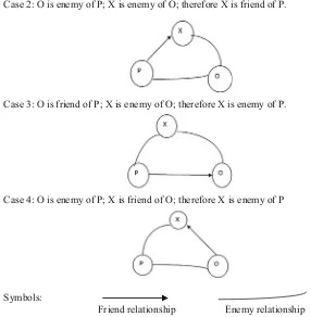
Case1: O is a friend of P; X is a friend of O; therefore X is a friend of P with large probability.

Case 2: O is enemy of P; X is enemy of O; therefore X is friend of P.

Case 3: O is friend of P; X is enemy of O; therefore X is enemy of P.

Case 4: O is enemy of P; X is friend of O; therefore X is enemy of P

Symbols:

Friend relationship Enemy relationship

Fig. 4.1 Structural relationship model for users

(49)

4.4 Proposed System

To increase the sales and to attract the customer, it is necessary to improve the performance of the recommender system. Drawbacks present in the collaborative filtering method are solved by using the neighborhood algorithm by considering the product rating as well as the seller rating. The product rating is given by the customer or the end user who buys that product. Rating is given based on the quality of the product and the satisfaction of the end user on the product. By using the product rating, the customer can easily judge whether the product is good or bad.

The seller rating is given a group of people. They include the admin of the E-commerce Web site, various sellers, manufacturer of the product, and many more. The seller rating is given based on the packing, delivery, and quality of the product. By using the seller rating, the admin can monitor his sellers, and at the same time, it will help the customer to understand the shipping details and quality in a very clear manner. Seller rating is computed by calculating the average of all the seller ratings, user ratings, and manufacturer ratings. When only product rating is considered for recommending the products, the following problems have occurred:

(50)

1. The cold-start problem 2. Loss of neighbor transitivity 3. Sparsity

To solve these three problems, the neighborhood algorithm with integrated rating approach has been introduced. The cold-start problem can be avoided by including a feedback form in the application where the user can enter his preferences. Based on the feedback, the products are recommended to the user when he enters into the application for the first time.

A. System Design

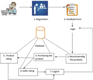
The integrated recommendation using product and seller rating overcomes the problem of cold-start problem, data scarcity problem, synonymy, and single attribute consideration. The process of the application is elaborated in Fig.4.2.

B. Algorithm

INPUTS:

USER {user1, user2… usern}: a set of users present in the application system. PRODUCT {P1, P2… Pn}: a set of products present in the database.

PRODUCT_PURCHASE {PP1, PP2… PPn}: a set of purchased products by useri. FEEDBACK {F1, F2…. Fn}: a set of feedback forms for each useriin USER. P_RATING {user1, user2… usern}: set of product ratings given by user. S_RATING{user1, user2… usern}: set of seller ratings given by user. FRIEND{user1, user2… usern}: set of similar users for usertarget. ENEMY{user1, user2… usern}: set of dissimilar users for usertarget. usertarget:target user to whom the products are recommended.

Similarityproduct: similarity between two users when only product rating is consid-ered.

(51)

The algorithm first allows the user to register in the system, and upload a feedback form for several attributes if the user is login at first time. Then, it checks whether the user login is for the first time or not. If it is for the first time, then the algorithm invokes the feedback_recommendation method. If the user login is not for the first time, then the integrated_recommendation method is called.

The feedback_recommendation method displays the products to the customers based on the feedback form. The integrated_recommendation method first sets a threshold value p or enemy. USERi is the user set, friend is the similar users set, and enemy is the dissimilar users set present in the system. Then, for the target user similarity is calculated for each user present in the system. If the similarity computed is less than the threshold value, then the user is kept in the enemy set of the target user; otherwise, the user is kept in the friend set. After classifying the users into different sets, the same procedure is repeated by considering the seller rating. Finally, the mean of both the similarities is calculated, and if the similarity is greater than the 60%, the products are recommended to the target user.

1. Feedback-based recommendation

(52)

2. Integration recommendation using neighborhood algorithm.

2.1. Calculating similarity using product rating

Determine user target’s “possible friends” through “enemy’s enemy is a friend” and “enemy’s friend is an enemy” rules. The similarity between the target user and normal user is computed by using the product rating.

2.2 Calculating similarity using seller rating

Determine user target’s “possible friends” through “enemy’s enemy is a friend” and “enemy’s friend is an enemy” rules. The similarity between the target user and normal user is computed by using the seller rating.

3. Integration and recommendation

The mean value of similarities calculated in the above two modules is calculated, and if the mean value is greater than 60%, then the algorithm recommends the useri products to the target user.

Example

Let us consider an n*m matrix for each customer Ciwhich consists of the product IDs purchased by Ci, his/her product and seller ratings on the purchased products.

Ci

In the above matrix, the Ci represents the customer IDs,P1,2…mrepresents the

product IDs,PRidenotes the product ratings, andSRidenotes seller ratings wherei

∈_{{1, 2. 3,…}_n_}.

(53)

C4

• _{set I represents the common product items that were rated by}_C_target_and_C_i_where

C denotes the customer.

• I_targetandI_idenote the product item sets that were rated by usertargetand user_i. • R_target-_jandR_i_-_jrepresent usertarget’s ratings andC_i’s ratings on product itempro_item. • R_targetandR_i denote the average rating scores of all the product items rated by

CtargetandCi.

1. Calculate the similarity betweenCtargetandC1using Eq. (4.1).

Sim(Ctar,C1) (4

2. Calculate the similarity between the users using the seller rating using Eq. (4.1).

Sim(Ctar,C1)

Now, the mean value of both the similarities calculated through step 1 and 2 is:

Mean(0.71 + 0.8)

2 0.78

Therefore, the similarity between theCtarandC1is 78%. Since it is greater than 60%,C1is considered as friend ofCtarand productP3is recommended toCtar. C. Physical Model

(54)

Fig. 4.3 Neighborhood relationship between customers

Fig. 4.4 User and product level for integrated recommendation

(55)

Fig. 4.5 Registration page

4.5 Experiments and Results

The whole process of Web recommendation using integration rating is for predicting online purchase behavior of user which is displayed in this paper. In order to describe the online purchase behaviors comprehensively, six features are extracted from the seven fields of the raw data with SQL Server.

In Fig.4.5, the application allows the customer to register his details which is done only once. The details of the customer are stored in the database when the user clicks on registration button.

In Fig.4.6, feedback form consisting of four fields, brand, color, prize, and range, is given to the customer. The feedback form appears after the registration page. The main purpose of including the feedback form is to recommend the products to the customer when he enters into the application for the first time. The entire data is stored in the database when the customer clicks on upload feedback button.

In Fig.4.7, the login page for the customer has been created. The login page will start a session for the customer, using which he/she can purchase the products.

In Fig.4.8, the products present in the database are displayed based on the feed-back form. The feedfeed-back-based recommendation is used when the user enters the application for the first time. The customer can give the product rating in this page. This reduces the problem of cold-start.

(56)

Fig. 4.6 Feedback form

Fig. 4.7 Login page

In Fig.4.10, the list of purchased products for a particular customer is displayed in this page. The customer here can give the seller rating based on some factors, such as packing, delivery.

(57)

Fig. 4.8 Recommendation based on feedback form

Fig. 4.9 Connecting to the Flipkart

rating. And in the integrated recommendation, the products are displayed based on both the product and seller rating. The more accurate results are shown in integrated recommendation than in product recommendation.

(58)

Fig. 4.10 Giving the seller rating

Fig. 4.11 User second-time login

(59)

Table 4.1 No. of

recommended products using product rating

No. of users No. of products recommended

0 0

No. of users No. of products recommended

0 0

web recommendaƟon using product raƟng

4.6 Conclusion and Future Work

(60)

inte-Fig. 4.13 Web

web recommendaƟon using integrated raƟng

No of recommnded products

grated recommendation approach where the product and seller rating are considered as two parameters for calculating the similarity between the target user and the exist-ing user. The recommended products are accurate when the integrated approach is implemented with selected feature. In future work, we will develop an automated sim-ilarity threshold setting method to satisfy the requirements of different E-commerce users.

References

1. Thotharat N (2014) Thai local product recommendation using ontological content based filter-ing. Business Comput Dept Fac Manage Sci

2. Liu X, Li J (2014) Using support vector machine for online purchase predication. IEEE Trans 3. Trinh G (2013) Predicting future purchases with the poisson lognormal model. IEEE Trans 4. Jamalzehi S, Menhaj MB (2016) A New similarity measure based on item proximity and

closeness for collaborative filtering recommendation. IEEE, 28

5. Cai Y, Leung H, Li Q et al (2015) Typicality-based collaborative filtering recommendation. IEEE Trans

6. Zhong Y, Fan Y, Huang K, Tan W, Zhang J (2014) Time-aware service recommendation for mashup creation. IEEE Trans Serv Comput 8(3):356–368

7. Zheng Z, Ma H, Lyu MR, King I (2013) QoS-aware web service recommendation by collabo-rative filtering. IEEE Trans

8. Kavinkumar V, Reddy RR, Balasubramanian R, Sridhar M, Sridharan K, Venkataraman D (2013) A hybrid approach for recommendation system with added feedback component. IEEE 9. Chiu C, Wang E, Fang Y, Huang H (2014) Understanding customers’ repeat purchase intentions in B2C E—commerce: the roles of utilitarian value, Hedonic Value and Perceived Risk. Inf Syst J 24(1):85–114

10. Tian Y, Ye Z, Yan Y, Sun M (2015) A practical model to predict the repeat purchasing pattern of consumers in the C2C e-commerce. Electron Commerce Res 15(4):571–583

(61)

12. Lin S, Lai C, Wu C, Lo C (2014) A trustworthy QoSbased collaborative filtering approach for web service discovery. J Syst Software 93:217–228

(62)

Chapter 5 A Quantitative Analysis of Histogram

Equalization-Based Methods on Fundus

Images for Diabetic Retinopathy

Detection

K. G. Suma and V. Saravana Kumar

Abstract Contrast enhancement is an essential step to improve the medical images for analysis and for better visual perception of diseases. Fundus images help in screening and diagnosing the diabetic retinopathy. These images must be enhanced in contrast, and the brightness should be preserved to view the features correctly. In addition, the fundus image should be analyzed by Histogram Equalization-based methods to detect DR abnormalities effectively. In this paper, various image enhance-ments based on Histogram Equalization have been reviewed on fundus images and the results are compared using image quality measurement tools such as absolute mean brightness error to assess brightness preservation, peak signal-to-noise ratio to evaluate the contrast enhancement, entropy to measure richness of the details of the image. The proposed results show that the Adaptive Histogram Equalization is the best enhancement method which helps in the detection of diabetic retinopathy in fundus images.

Keywords Diabetic retinopathy

_·

Fundus images

_·

Histogram Equalization Normalization

_·

Brightness preservation

_·

Contrast enhancement

_·

Entropy

_·

Image quality measurement

5.1 Introduction

Image enhancement is a preprocessing step in image or video processing that is mainly used to increase the low contrast of an image [1]. Contrast enhancement adjusts dark or bright pixels of an image to bring out the hidden feature in that image. Digital medical images help the professional graders in screening and diag-nosing the diseases. Diabetic retinopathy (DR) is a complication of diabetes mellitus that affects the vision of the patient and sometimes leads to blindness. Fundus image captured by fundus camera helps to analyze the anatomy of retinal part of an eye (blood vessels, macula, fovea, optic disk) and is used to monitor the abnormali-ties of diabetic retinopathy (microaneurysms, hemorrhages, soft and hard exudates, neovascularizations) [2].

Ch. Satyanarayana et al.,Computational Intelligence and Big Data Analytics,

SpringerBriefs in Forensic and Medical Bioinformatics, https://doi.org/10.1007/978-981-13-0544-3_5

Computational Intelligence and Big data Analytics Application in Bioinformatics pdf pdf

T E C H N O LO G Y 

FORENSIC AND MEDICAL BIOINFORMATICS

Ch. Satyanarayana

Kunjam Nageswara Rao

Richard G. Bush

Computational

Intelligence

and Big Data

Analytics

SpringerBriefs in Applied Sciences

and Technology

Forensic and Medical Bioinformatics

Ch. Satyanarayana

Kunjam Nageswara Rao

Richard G. Bush

Computational Intelligence

and Big Data Analytics

Applications in Bioinformatics

Contents

Chapter 1

A Novel Level-Based DNA Security

Algorithm Using DNA Codons

·

·

·

·

·

1.1

Introduction

1.2

Related Work

1.3

Proposed Algorithm

1.3.2

Decryption Algorithm

1.4

Algorithm Implementation

1.4.1

Encryption

1.4.2

Decryption

1.5

Experimental Results

1.5.1

Encryption Process

1.5.3

Padding of Bits

1.6

Result Analysis

1.7

Conclusions

References

Cognitive State Classifiers for Identifying

Brain Activities

·

·

·

2.1

Introduction

2.2

Materials and Methods

2.2.1

fMRI-EEG Analysis

2.2.2

Classification Algorithms

2.3

Results

2.4

Conclusion

References

Multiple DG Placement and Sizing

in Radial Distribution System Using

Genetic Algorithm and Particle Swarm

Optimization

·

·

·

·

·

_{FORENSIC AND MEDICAL BIOINFORMATICS}

_·

_·

_·

_·

_·

_·

_·

_·

_·

_·

_·