Evaluating the Italian training on the job contract (CFL)
G. Tattara* and M. Valentini*
[email protected] and [email protected]
Abstract. The “Contratto Formazione e Lavoro” (CFL - training on the job contract) is a fixed term contract aiming at reducing unemployment and supporting the training of young Italian workers. CFL was introduced 20 years ago, in a period of severe unemployment, and basically extended some of the significant characters of the apprentice contract to 29 years of age, set a definite term, 24 months, for the training period, and provided incentive for employers to hire young people under the program reducing hiring, firing and labour costs.
Using the introduction of the CFL contract as an exogenous innovation and exploiting the reform of the program over time (e.g. artisans were guaranteed higher fiscal benefits for a longer period in respect to non artisans) the effect of CFL on the Italian labour market is discussed and evaluated. Difference in difference technique together with matching method are used in order to establish if CFL has improved Italian young workers hiring chances.
Our estimates support a positive CFL effect on employment at the introduction of the program, while the subsequent reforms bear effect on firm’s probability to enter CFL program. In such a way our study questions some previous results bearing no evidence of a significant positive policy effect for this program.
Keywords: policy evaluation, differences in differences-matching, regional labour market, panel data.
JELclassification: E64, J38, J48, J58, J68, R23.
1.
Introduction
In the early eighties the situation of the Italian labour marked drastically deteriorated with the number of unemployed rising from around 300.000 to 800.000 in less than five years (Cigs included). The unemployment wave was accompanied by a deep segmentation in the labour market, with severe unemployment among young people and had a dramatic increase in the South. To overcome the unemployment problem an active labour market policy was devised and great emphasis was placed on Contratto Formazione e Lavoro (CFL – Training on the Job Contract), a significant innovation in the legislative Italian labour market framework providing incentive to the hiring of young people as a training initiative.
CFL was a significant active labour market instrument. The program began in the mid eighties, affected many firms and workers, and lasted until the end of nineties. Its declared goals were to reduce youth unemployment and contemporaneously upgrade young workers’ human capital. In order to spread this kind of contract, the policy maker granted a strong fiscal rebate to firms adhering to the program, and conceived CFL as a fixed term contract, so to avoid firing costs to the firms. Both the fiscal benefits connected to the CFL program and the eligible categories varied through time.
Up to now the CFL evaluation has been constricted due to the unsatisfactory data situation. Only a few studies evaluated some aspects of the contract and they do not address directly the question of the CFL effect at the contract launching in 1985.
Our paper presents a microeconomic evaluation of the CFL in two Veneto provinces, focusing on the effects on the participating individuals and taking into account several sources of heterogeneity. The territorial choice has been constrained for data availability, but Veneto looks an
*
interesting case study as well, because of the prevalence of small size firms, and it is well known that these firms have been particularly active in entering the CFL program.
The estimation is based on a panel derived from the social security dataset built at the University of Venice. It contains information on all participants in the CFL program in the private sector, in the two provinces of Treviso and Vicenza, for the years 1985-1996, that amounts to around 40.000 firms hiring 400.000 employees as CFL (over a population of about 90.000 firms and 850.000 employees).1
Program evaluation is defined as the use of research to measure the effects of a program in terms of its goals, outcomes, or criteria2. Evaluative research is required in order to improve or legitimate the practical implications of any policy-oriented program. Behind the seemingly simple question of whether a program works are hidden a host of other more complex issues. The starting question is, what is a program supposed to do? It is often difficult to answer this point directly and the most difficult part of the evaluation procedure lies in determining whether it is the program itself that is doing something. There may be other events or processes that are really causing the outcome, or preventing the expected outcome. Many times, due to the nature of the program, the evaluation procedure fails to determine whether the program itself, or something else, is the ‘cause’ of the outcome.
The reason that makes evaluation difficult is due to the fact researcher have not simultaneously factual and counter-factual outcomes for each treated unit. Given this missing data problem one of the main reason that evaluation cannot determine causation involves self-selection. That is, people select themselves to participate in a program. For example CFL program is directly addressed to firms; some decide to participate and other, for whatever reason, do not participate. It may be that firms taking part in the program are the firms that are the most determined to increase employment, or that have the best support resources, thus allowing more people to be hired and to take part in the recruitment program. Participants are somehow different from non-participants, and it may be this difference, not the program, that leads to a successful outcome for participants i.e. to the employment increase.3
Section 2 describes the CFL program, its structure and the relevant reforms through time. In the present study CFL is considered only in relation to the goal of promoting youth employment; other possible benefits (skills, training on the job etc.) are not considered. Section 3 introduces the evaluation problem and the methods used in this paper. Section 4 describes the data-set and investigates through both descriptive methods and econometric analysis the CFL impact. First we evaluate the effect of the CFL program at its introduction, the impact effect. Second, exploiting the variations in the eligible category over time, we discuss if the firms that have already hired CFL workers revise their past decisions and if the revision leads to a consistent reduction of CFL hirings. Section 5 concludes.
2.
CFL’s settings
CFL is a fixed term contract introduced by law 863/84, whit a maximum duration of 24 months, not renewable.4 The program goal is to decrease unemployment among young workers and, at the same time, to train them, easy their entrance into the labour market and make their career more stable and qualified, as provisions to transform CFL into tenure are provided.
1
This was made possible by the courtesy and skill of dott. Antonino Travia and signor Francesco Morabito of the INPS.
2
CFL has not to be confused with cost benefit analysis that considers the costs of the intervention and the received benefits.
3
If program could, somehow, use random selection, then researchers could easily determine causation. That is, if a program could randomly assign firms to participate or to not participate in the program, then, theoretically, the group of firms that participates would be the same as the group that does not participate, and an evaluation could ‘rule out’ other causes.
4
CFL provides fiscal benefits to the firms hiring young people under the program, materializing in social security contributions substantial rebates. Eligible firms are public firm and private firms, which did not record massive firings at the application date and whose training project (training timing and pattern) is endorsed by the Regional Commission for Employment.
At the program introduction, the fiscal fee on labour was limited to 5000 lire per week-per capita (about 2.58 euro) and the bonus was basically extended one year after the contract expired if the worker was regularly hired. The law 291/88 drastically curtailed the rebate to the 50% of the fiscal benefit, subsequently decreased to 25% by the law 407/90 since 1/1/91 (for firms of trade and tourist sector with less than 15 employees the rebate was maintained at 40%) (Tab. 1). The full rebate has been maintained all along for artisan firms. Additionally CFL allowed firms to hire directly their workers, without inquiring the Italian “Ufficio di Collocamento”, which means hiring from a pool of declared unemployed and entrepreneurs evaluated very favourably this possibility. Subsequently by the law 223/91 direct hiring was extended to all firms and the advantage of hiring under the program was lost.
At the beginning workers eligible under the CFL program were young people between 15 and 29 years of age.5 The law 451/94 loosed the boundaries and changed the eligibility range to between 16 and 32 years of age.6 The Law 451/94 extended CFL to liberal professions, association and research centres7 and created two kind of CFL aiming at: A) providing new skills (intermediate and high skills); B) easing the hiring process through a practical work experience that fits the worker skills and capacities to the production environment and to the organisational structure of the firm. CFL of the first type extends up to 24 months, CFL of the second type up to 12 months. Eventually law 451/94 allowed the rebate to be maintained one year after the contract transformation in case of CFL of the first kind, while in case of CFL of the second kind the rebate was applied only if the contract was transformed. Southern regions continued to enjoy full rebate.
Since 1991 (L. 407/90) eligible firms were requested to have hired with a tenure contract, during the two preceding years, at least 50% of the terminated CFL.8 This percentage has risen to 60% by L. 451/94.
Another important contract run parallel to CFL, the apprenticeship contract. Apprenticeship aims at training young workers in order to qualify them. Eligible workers are young people, between 14 and 20 years of age (for artisan firms the upper limit was extended to 29 years of age by law 56-28/2/87). The same law 56/87 allowed all firms to hire directly their apprentices, without inquiring the Italian “Ufficio di collocamento”. Previously Italian firms - except artisans and firms with less than 10 employees - were allowed to hire directly only 25% of their apprentices. The length of the apprenticeship contract is not inferior of 18 months and does not extends over five years; the preceding periods concerning the same activity with other employers may be cumulated.
Tab. 1: Rebates on Total Social Security Contributions by Category.
Year South, artisans, high
unemployment area
Trade-tourism firms with
less than 15 workers All other firms
1/5/84-31/5/88 About 98% About 98% About 98%
1/6/88-23/11/90 About 98% 50% 50%
24/11/90-31/12/90 About 98% 50% 25%
1/1/91-… About 98% 40% 25%
5
32 years old for the South of Italy and the North-Italian regions with an unemployment rate higher than national average.
6
Starting date was 19/11/93 (D.L. n.462 of 18/11/93 and D.L. n. 32 of 17/1/94), moreover regions of the South of Italy until 31/12/97 benefited from a higher age limit.
7
The last was included by law 196/97.
8
3.
Evaluation problem
The standard evaluation model assumes that individual can choose between two states, i.e. either participating in a certain labour market program or not. The individual has two potential outcomes, where Y1i is a situation with treatment and Y0i is a situation without treatment. Use Di as a dummy variable representing the treatment status, assuming value 1 if individual i has been treated and 0 otherwise. The impact of the program for i-th subject is Y1i-Y0i. As the same individual is not observable in both states at the same time, we have to deal with a counterfactual situation (that amounts to a missing data problem). What is observable is:
i i i
i
i DY D Y
Y = 1 +(1− ) 0 (1)
Let Xi denote the individual characteristics, the observables are Yi,Di,Xi.
In the simplest of all the worlds, treatment can be assumed to be constant across individuals: i
Y1
=
γ -Y0i for any i, and in such a simplified context the only source of bias that one has to worry about is selection bias.
More realistically the treatment effects can vary across individuals:γi =Y1i-Y0i, i.e. outcome variations might depend on systematic differences among individuals of observables and/or unobservable characteristics. Broadly speaking every parameter depending on the joint distribution of Y1iand Y0i can not be estimated, in particular we can not estimate E(Y1i-Y0i)) because either Y1i or Y0i is missing but some characteristics of the (Y1i-Y0i) distribution can be identified under appropriate assumptions (Heckman et al.,1999; Blundell, Costas Dias, 2002). The evaluation literature has mainly concentrated on three moment of (Y1i-Y0i) distribution. The following three9 parameters depend on the marginal distribution of Y1i and Y0i:
1) The Average Treatment Effect (ATE): E(Y1-Y )0 or its conditional version E(Y1-Y |X)0 . ATE is defined as the expected gain from participating in the program for a randomly chosen individual;
2) The Average Treatment Effect on Treated (ATT): E(Y1-Y |D=1)0 or its conditional version
E(Y1-Y |D=1,X)0 ; ATT is the average gain from treatment for those that actually select into
the treatment;
3) The Average Treatment Effect on Untreated (ATNT): E(Y1-Y |D=0)0 or its conditional version E(Y1-Y |D=0,X)0 ; ATNT is the average gain from treatment for those that actually do not select into the treatment;
Since the underlying principles for studying any of these three parameters are similar, let’s concentrate on the sub-sample of the treated. Estimating this effect requires to make inference about the outcome that would have been observed for participants had they not participated. In non- experimental studies no such direct estimate is available. A basic assumption is required, the stable unit-treatment value. The assumption requires that the potential outcomes for an individual depend on its own participation only and not on the treatment status of other individuals and that whether an individual participates or not does not depend on the participation decision of other individuals. Both cross effects and peer effects are excluded.
The second parameter (ATT) can be written as:
9
)
The first term on the right-hand side is computed directly from data, whereas the second term estimation requires appropriate assumptions. For example the “naïve” estimator:
) particular circumstances, such as a random experiment, where the two populations (treated and untreated) are the same. On the contrary the estimator is biased any time different populations with different distributions are compared:
)]
In other words, the naïve estimator is made up by two components, respectively the true ATT component and the bias. As shown by Heckman et al. (1998) the bias can be split in three parts: the first component is due to the non overlapping support (the two population have completely different characteristics, X); the second, to the different distribution of X, within the two populations; the third, to the remaining differences in the outcomes, after controlling for the first two biases.
Heckman et al. (1997) have speculated that if the data on participants and controls are collected through the same questionnaire, all over the same local labour market, then the last bias component is the least important, so that, once the common support and the misweighting issues have been correctly addressed, the most of the bias disappears.
3.1 Differences in differences
Suppose a panel made by two populations, non treated and treated. The second population is made by individuals who switch treatment status over time, so that two outcomes can be observed for the same people, albeit not simultaneously but at a different point in time.
Label period t=t2 the date of the reform and t=t1 the earlier period. For every individual 1
it
The first two terms are observables and ATT can be identified only when the expression within square brackets is zero. Hence the identifying assumption of the Differences in Differences (DID) estimator is
(5) assumes that there is no difference in the trend outcome between non participants and participants when there is no treatment. In other words if treated and not treated are systematically different, this difference cannot change over time.
error term (Bell et al., 1999). Second, matching treated and untreated observations that have the same pre-treatment observable characteristics, and running a DID estimator over the matched observations. In such a case people who have the same characteristics are very likely to have the same trend.
The second case will be discussed in section 3.3. Let’s turn here to the first case. Label C the comparison group and T the target or treatment group T. The relationship between Y and the individual characteristics for the treated is written as10
it the T or C group. This would be a consistent estimator of γ if non-observables satisfy the following relation
The above condition allows a macro trend effect; but the macro effect is the same across the target and the comparison group, as pointed out in (5). In order to make this assumption more plausible the “DID regression adjusted” is run within some cells described by X, in order to reduce the unobserved heterogeneity (Cochran, 1968).
If each of the two groups is allowed to respond differently to the business cycle effect, the relation is
where the Kg acknowledges the differential macro-effect across the two groups. The DID
estimators consistently estimates γ (Bell, et al., 1999):
)
provides consistent estimates of γ.
10
3.2 Regression adjustment
The assumption is that the outcome is affected only by observables; in other words there is no selection on the non-observables. Label uDi the unobserved heterogeneity; selection on observables is written as
0 ) | ( ) , |
(u0i Di Xi =E u0i Xi =
E (12)
According to (12) once Xihas been taken into account, the error term, on average, is independent
of the treatment status, i.e. ui is a random sample for Di. Hence the naïve estimator on the residuals
can be used:
i i i
i D X u
Y =γ +β′ + (13)
Under the above mentioned hypothesis and under the classical OLS assumption, γ =ATT. Indeed (12) can be written as
i i
i X u
Y0 =β′ 0 + 0 (14)
i i
i X u
Y1 =γ +β′ 1 + 1 (15)
if (12) holds
X X
Y E X D
Y E X D Y
E( 0i | i =1, i)= ( 0i | i =0, i)= ( 0i | i)=β′ (16) now ATT(X)= E(Y1-Y |D=1,X)0 and substituting the above equation (16), ATT(X)= γ . In words
the regression adjustment overcomes the common support problem using linear forecast, and taking into account the X’s, is free from misweighting.
This method is straightforward and can be improved in order to allow for the heterogeneous impact and to account for the misspecification issues, but it relies on very strong assumptions.
3.3 Matching
Matching selects the untreated observations as close as possible to the treated ones in terms of observable characteristics. In other words matching “mimics” experimental data using observational data. Matching is based on the conditional independence assumption11 (CIA):
0
Y ||D|X (17)
conditioning on X, Y and D are independent. A weak version of CIA is required: )
, 0 | ( ) , 1 |
(Y0 D X E Y0 D X
E = = = . Given X, on average, the non-treated outcomes are what the treated outcomes would have been if they had not been treated.
Moreover matching assumes 1
) | 1 Pr(
0< D= X < (18)
11
if (18) holds for all X, then ATT, can be defined for all values of X. The meaning of (18) is that for each X, observations on both treated and untreated are available. This hypothesis is quite stringent in relation to the available observations, and is usually replaced by the common support assumption,X = X1∩X0.
Under these assumptions, ATT can be identified as:
∫
= =Each treated is matched by a not treated unit sharing the same individual characteristics.
To carry out matching estimation (19) we must match on a high dimensional X, i.e. we have to study high dimensional density. Rosenbaum and Rubin (1983) have shown that if CIA holds, then it is valid for any balancing score,12 b(X). Defining the propensity score, p(X), as the conditional probability of assignment to treatment
)
the propensity score is the coarsest balancing score and X is the finest. Putting altogether we can write
Hence matching on propensity score bears an unbiased estimate of ATT. A powerful result because only one dimensional density is needed in order to get the appropriate estimation.
In general after having run logit, probit or semiparametric estimation on pre-treatment variables X, the fitted values, p(X), are used in order to match treated and control units. Following Heckman et al. (1997) the form of the matching estimator can be cast in the following framework
X
where Q1i is function of the treatment outcome, and Q0i is function of the comparison group
outcome, W(i,j) is a weight with
∑
∈ (, )=1 Cj W i j and ω(i) is a weight that accounts for heteroscedasticity and scale. The notation (22) is general so to allow regression adjusted Y, or DID estimator. Matches for each participants are constructed by taking weighted averages over comparison group members. Matching can be performed within various strata to recover estimates relative to different subset of the population of interest (Heckman et al., 1997, Rosenbaum and Rubin, 1984). Matching estimators differ in the weight attached to the members of the comparison group (for a survey see Heckman et al., 1999).
Label C(pi) the set of untreated neighbours of the treated i, which has a propensity score
estimated value of pi, the nearest-neighbour matching estimator sets Q1i=Y1i, Q0i=Y0i, ω(i)=1/NT, method are available: with replacement or without replacement of the Xj (reusing or not Xj for other
matches).
12
A balancing score, b(X), is a function of the observed covariates X such that the conditional distribution of X given
b(X) is the same for the treated and the control units: X||D|b(X). The most trivial balancing score is X.
13
Nearest-neighbour matching use all the treated group, without caring about the effective distance between individuals i and j, but distance has to be set to the minimum. In order to avoid matching too different individuals, a pre-specified tolerance (calliper) can be imposed (Cochran and Rubin, 1973). Calliper matching requires = i − j <τ
j
i p p
p
C( ) min whereτ is the tolerance level.
“One to one matching” can be easily extended to the “smoothed matching”. For example, n-nearest neighbour matching considers as counterfactual the n closest control observations for each treated unit, instead radius matching considers all untreated observations which have a propensity score falling within a radius τ from pi: C(pi)= pi −pj <τ.
In the last two methods W(i,j)=1/NiC if j∈C(pi) and zero otherwise (NiCis the number of control unit matched with i-th treated observation).
Through the process of choosing and re-weighting observations, matching corrects for the first two sources of bias, and selection on non-observables is assumed to be zero. Compared to the regression method, matching is non parametric and therefore avoids the inconsistency due to misspecification and estimates over a common support only comparable individuals.
Heckman, Ichimura and Todd (1998) combine matching method and regression adjustment on the X. Their method extends the classical matching by utilizing information on the functional form of the outcome equations. This estimator can be considered as a compromise between the fully nonparametric approach and a parametric model.
Regression-adjusted matching is performed by the following procedure. Assume a conventional econometric model for outcomes in the non-treatment state that is additively separable in the observables and unobservables (14); estimate the component of
)
E β using partially linear regression methods. Before
estimating ATT by matching methods (22), Xβˆ0 are removed from Y0 and Y1 by setting difference between before and after treatment matching estimates, allows to get ATT combining matching and DID (Heckman et al., 1998). Obviously the CIA assumption needs to hold not on level but on differences:
)
and under additive separability of the errors and index sufficiency the condition becomes )
From the econometric point of view the DID-matching “is an attractive estimator because it permits selection to be based on potential programme outcomes and allows for selection on unobservables” (Heckman et al., 1997).
4.
Main results
4.1 Data
plant and each single individual employed in the private sector (no state and local government, with few exceptions) except for farm workers and people receiving no salary.
Inps data include register-based information on all establishments and employees that have been hired by those establishments for at least one day during the period of observation, independent of the workers place of residence.14 The unit of observation is the employer-day; such information is used to build a monthly history of the working life of each employee. Employers are identified by their identification number, which changes if ownership, in a strict sense, changes. This has been amended and any time more than 50% of all employees are taken over by the new legal employer, the employment spell is said to be continuing. Similarly, if there are short breaks in the employment spell, as long as the worker continues at the old employer, his spell is considered uninterrupted.15 CFL spells are clearly identified.
Data include all individual employment spells with an employer, of whatever duration, and this probably results in a lot of very short spells. Although short spells characterize the average job, they are concentrated at workers young age, while long spells characterize the mature worker current experience. We keep all employment size in our data set, because our territory is characterized by a multitude of very small units (establishments with ≤ 5 employee account for almost 12% of the total manufacturing employment).
Veneto labour market has been characterized, since a decade, by almost full employment and by a positive rate of job creation in manufacturing, before a negative national rate. It is a dynamic territory based on manufacturing, with a large population of small firms; the average establishment size is 12 employees. The stock of manufacturing workers in the two Veneto provinces of Treviso and Vicenza has varied between 194.000 employees at the early eighties and 233.000 employees in 1996, with a yearly positive average rate of variation of 1.4%. The average rate of growth in employment is the result of a marked increase of white collars and women.
Employers are classified according to the three-digit ATECO 1981 standard classification. The database has records on establishments and workers from 1975 to 1997.
4.2 Descriptive analysis
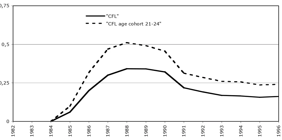
Figure 1 depicts the share of workers hired under the CFL program in the private sector over the total yearly hiring flows, for the eligibility age classes (15-29 years of age).16 More than one third of the new hirings in the eligibility age classes were CFL. Indeed, the group 21-24 seems more sensible to the program from the very beginning; only for artisan firms after 1987 this age cohort was also eligible to the apprenticeship contract and this might have raised the employment rate during the last part of the period. CFL flows relevance reflected only slowly on workers stock, but in 1989-90 one quarter of our employee stock was made up by people with a CFL contract.
14
The entire working life for all employees that have worked at least one day in Treviso and Vicenza, has been reconstructed, considering the occupational spells out of Treviso and Vicenza as well.
15
A ‘cleaned’ social security archive has been used. The engagements/separations and the creations/destructions that are due to a change in the unit that pays the social security contribution not matched by a corresponding change of the working population assessed at the establishment level are defined as ‘spurious’ and have been deleted. This has lead to a reduction of 9% of total engagements and separations in manufacturing. This procedure is common practice among people working with social security data.
16
Figure 1. Workers Hired as CFL over the Yearly Hiring Flows.
0 0,25 0,5 0,75
1
9
8
2
1
9
8
3
1
9
8
4
1
9
8
5
1
9
8
6
1
9
8
7
1
9
8
8
1
9
8
9
1
9
9
0
1
9
9
1
1
9
9
2
1
9
9
3
1
9
9
4
1
9
9
5
1
9
9
6
"CFL"
"CFL age cohort 21-24"
The CFL share had a very rapid increase just after program introduction in 1985 and stayed at high levels till 1989. Indeed the first reform with the severe fiscal bonus reduction marked a set back on the CFL diffusion and CFL subsequently stabilized at half of the level reached at its peak. The CFL flows share the same wavelike movement of the hiring flows, following the cycle; CFL gaining importance when the economy peaked in 1989-90, declining when the economy declined in the early nineties and timidly recovering with the economic recovery of the mid nineties.
According to economic theory, fiscal rebate on young workers induces the firms to replace capital with labour, hiring specifically young workers that are now less costly. For the same reason we expect young workers to replace older workers as the relative cost has significantly shifted in favour of the first category. The two movements reinforce each other and lead to a relative increase in the young workers employment ratio under the program. An opposite effect is expected when the CFL rebate diminishes.
Figure 2. Employees over Residents by Age Cohort According to Eligibility. Index 1986=1.
0,85 0,95 1,05 1,15
1983 1984 1985 1986 1987 1988 1989 1990 1991 1992 1993
30-32-NON ELIGIBLE 21-24-ELIGIBLE 25-29-ELIGIBLE
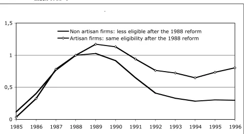
Figure 3. CFL over Stock for Eligible Age Cohort. Age 21-29 till 1993, and 21-32 since 1994. Index 1988=1
.
0 0,5 1 1,5
1985 1986 1987 1988 1989 1990 1991 1992 1993 1994 1995 1996
Non artisan firms: less eligible after the 1988 reform Artisan firms: same eligibility after the 1988 reform
firms that have, as a result, a much younger employment stock. But of course the employment result embeds the effect of the employment cycle affecting differently artisan and non-artisan firms.
4.3 Econometric analysis
4.3.1. The impact effect
The Average Treatment Effect on the Treated estimates the average employment gain from treatment for firms that actually select into treatment. The dependent variable is the number of employees at the firm level. Treated firms are compared17 with non treated firms both in 1986 and in 1985. Untreated firms are defined as firms that never entered the CFL program.
A common assumption underlying the estimation strategy is the general equilibrium hypothesis, i.e., the program must not affect the control group.18 In actuality this assumption looks reasonable. Although CFL in the eighties was a widely diffused practice, a large amount of young workers was available for hiring by the non treated; moreover we assume that CFL did not affect the economic behaviour of not treated firms.
The crucial question in evaluating the program is to make clear if CFL promoted employment growth over the period or if CFL is just “another name” for people who, in any case, would have been hired or who were already employed. Firms participating in the CFL program were possibly self-selected – firms more prone to growth than the average firm - and evaluating the program economic return requires accounting for the non-random assignment of firms into the treated and untreated status.
The CFL exposed age group, from 15 to 29 years of age, has been limited to the range 21-29 and split into two parts: the 21-24 and the 25-29 age groups, in order to separate the program influence on the younger workers and on the more skilled workers. Workers are clustered according to the birth date. The panel excludes firms that are born or have died in the years under consideration, so the possible stock variation due to the natural process of firm’s birth and death is ruled out. Monthly level stocks have been preferred to the more common yearly stock, because firms start the CFL program continuously and because seasonality for young workers is quite strong. ATT is estimated over a period of 12 months from the CFL initial date in order to avoid capturing temporaryvariation of the eligibles (tab.2).
Tab. 2: Evaluation Prospect and Treated-Untreated Number.
Pre-treatment period under evaluation Treatment period under evaluation
i-12 … i-1 i: January,…, December, 1986 … i+11
Pre-treatment month used for logit Moth when firm entered CFL program
Firms with CFL between 21-24 years old. Treated: 1072 Untreated: 14308 Firms with CFL between 25-29 years old. Treated: 396 Untreated: 14308 Firms with the same characteristics are compared through the p-score matching method. An iterative procedure that accounts for different starting months has been devised: firms are pooled according to the month in which they adhered to the program and a logit model for each group has been estimated on the following “pre-treatment” (i.e. one month before, tab. 2) exogenous explanatory variables:19 size, sector, industrial area dummies, firm age, number of males,
17
CFL started in 1985 but only few firms adhered, thus the program is evaluated since 1986.
18
For example using as counterfactual the age group 33-34 would get biased estimates as there might have been a substitution effect between the eligible and the non eligible group.
19
collars (as proxy for more capital or labour intensive firms), apprenticeships (as proxy for firm inclination to use fixed term contract and training contracts), eligible workers for the CFL and its variation. In order to capture non-linearity, interaction and second order terms are allowed for. Yearly variation of eligible employees has been introduced in order to face the self-selection problem. Lagged employment in fact forecasts the future behaviour of the treated as far as employment is concerned and is independent from the CFL effect (selection independence).20 The autoregressive estimate of the yearly variation of the eligibles is reported in table 3. The variation of eligibles on its most recent past is estimated by simple OLS over the period and the coefficient of the lagged variable is significantly close to 1 with a high R2.
Tab. 3: Results of AR(1) Model for the Yearly Variation of Eligible Workers lagged yearly variation of eligibles
(Std. err.)
.9591724 (.0005126)
Adj R-squared 0.9049
The p-score21 is computed for each starting month, and treated and untreated firms with the p-score as close as possible and which belong to the same month of observation are matched. The calliper nearest-neighbour matching with a tolerance under 1% imposes a common support and excludes less than 5% of the treated population.22 Seasonality is dealt with by matching firms within the same month and taking the year differences (tab. 2). Finally the ATT estimator (DID -matching estimator) is computed as difference between the two yearly variation weighted averages. In the table 4 averages of some pre-treatment variables for treated and untreated firms which employed the two eligible worker cohorts are reported. The matching procedure performs quite well; indeed in terms of average dimension, number of artisan, average number of apprentices, and average yearly variation of eligible cohort, no significant difference between treated and untreated firms is perceivable (last two columns).
Tab. 4: Balancing Test for some Pre-treatment Variables.
Untreated average value Difference treated-untreated Cohort group
Variables 21-24 25-29 21-24 25-29
Size (std. err.)
20.31966 (1.261502)
23.61236 (2.325517)
1.294596 (1.784033)
-1.058989 (3.288777)
One year cohort variation (std. err.)
.0651042 (.0531908)
-.0484551 (.0569217)
.0159505 (.0752232)
-.0189607 (.0804995)
Artig (std. err.)
.3195801 (.0145955)
.3204588 (.0248215)
.0026855 (.0206412)
.0053839 (.0351028)
Apprentices (std. err.)
1.355062 (.0729959)
1.333801 (.1206571)
-.0142415 (.1032317)
.048221 (.1706348)
By extending the matching procedure into the past, the dependent variable appears balanced over the previous period. Table 5 shows the number of employees for the pre-treatment period. The eligible stock level is only slightly different between treated and not-treated firms.
20
The firm dimension variable has to be matched with great care as we do not want to confuse the impact effect with a different size issue. Assume we are comparing two firms, the first is untreated and has size 10, the second has size 100 and is treated, now figure out business cycle is positive and induce firms to increase size of 1%, it means just for business cycle we get treatment effect equal to (110-100)-(11-10)=9.
21
As said before looking at one particular starting month, we estimate one month before (pre-treatment) one p-score for each firm, and this value is constant for all temporal observation of the same firm.
22
Exploiting the different month of adhesion to the CFL program a possible “Anshefelter’s dip” is tested, i.e. assume that firms which have registered - pre-treatment - a decline in the number of their employees are selected so that the subsequent increase might be attributable to the “dip” and not to the program. The difference of the eligible worker stock between treated and untreated is, on average, statistically constant over time (about 0.2) and there is no evidence of any “dip” able to explain the employment increase for the firms entering the program (Table 5. A “dip” would have required a negative pre-treatment difference between treated and untreated);
Tab. 5: Pre-Treatment Differences Test on the Employment Level, in Matched Treated-Untreated Firms.
1985 1986
21-24 25-29 21-24 25-29
Matching differences (std. err.)
.1655273 (.0680191)
.2688827 (.1422469)
.2540971 (.0962501)
.2636726 (.1993668)
The CFL impact is quite strong (tab. 6). On average each treated firm hired one young worker more than not-treated firms. The outcome is very similar for the two age cohorts.
From descriptive evidence we know that the employment ratio for the age cohort 21-24 has increased more than the employment ratio for the subsequent cohort. The reason is quite simple: the total effect depends on two factors, the first is ATT, in other words the number of new eligible workers that each treated firms hired on average in relation to the not-treated firms, the second is the number of tread firms. The first component is almost the same between the two age cohorts, but the number of treated firms hiring people in the age cohort 25-29 is less than half the number of firms hiring people of the 21-24 age cohort (tab. 2), as CFL acted really as an entry level contract in the labour market.
Tab. 6: Estimated Effect of the CFL on the Two Eligible Cohorts by DID-Matching.
21-24 25-29
γDID
-matching (bootstrap std. err.)
1.101183 (.0228328)
.9996684 (.0235885)
During 1987 the eligible age for apprenticeship was extended from 20 to 29 only for artisan firms and this can affect out ATT estimate as young people employment growth might depend on apprenticeship extension and not on CFL program. Since the new apprenticeship law concerned only artisan firms and this kind of firms is balanced between treated an untreated, and given that also the number of a apprentices is balanced (tab. 3), then the apprenticeship extension is orthogonal to CFL program and is not likely to affect our results.
Tab. 7: Estimated Effect of CFL on other group by DID-matching
21-24 21-29 15-20 cohort
(std. err.)
.1576029 (.0226783)
.2682779 (.038752)
30-32 cohort (std. err.)
-.0024007 (.0112958)
-.0031796 (.0158533)
4.3.2 The CFL Reforms.
CFL reforms were introduced in the middle of 1988 and at the beginning of 1991. Since June 1988 and since January 1991 the fiscal rebate diminished over the previous level by 50% for non-artisans (treated) leaving the complete benefit to non-artisans (non-treated). The Average Treatment Effect on the Treated estimates the average eligible employment variation due to program reform for firms that were entitled to lower fiscal benefit. The dependent variable is the employees stock, and treated and non-treated are artisan and non-artisan firms, both adhering to the program, hence DID is used having artisans as the control group. The exercise is basically different from the previous one, because treated and non treated firms (non artisan and artisan) are now “exogenously” determined by the program.
The basic problem is heterogeneity between the treated and the control group, i.e. a problem of diversity. Observable heterogeneity is controlled by matching procedure. Artisan and non-artisan firms differ primarily in size and sector so that matching loses about half of treated firms. Moreover these two kind of firms are quite different, even after matching, at least in term of their behaviour along the business cycle; such heterogeneity23 needs to be faced and is taken into account using the regression-adjusted matching.24
Regression-adjusted matching makes use of additional variables in order to face the inter-temporal heterogeneity that biases ATT. In particular to account for the different reaction to the business cycle by the treated and the non-treated, the number of non-CFL hirings is considered. Indeed hirings are strongly pro-cyclical (Tattara-Valentini, 2004), treated (non artisan firms) and non treated (artisan firms) have a different cyclical behaviour through time – previous controls given – and hirings capture the variability that depends on the cycle for the two categories.
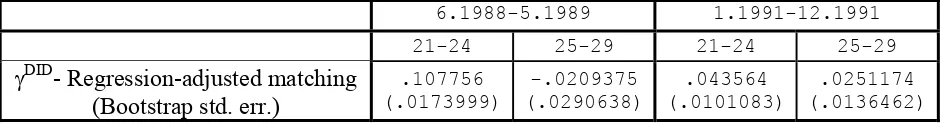
Table 8 reports the results of equation (22). The ATT estimates for the 25-29 age cohort shows no significant impact, and a slight positive impact for the 21-24 age group.25
Tab. 8: Estimated Effect of the CFL Reforms on the Two Eligible Cohorts by DID- Regression-Adjusted Matching.
6.1988-5.1989 1.1991-12.1991
21-24 25-29 21-24 25-29
γDID
- Regression-adjusted matching (Bootstrap std. err.)
.107756 (.0173999)
-.0209375 (.0290638)
.043564 (.0101083)
.0251174 (.0136462)
Among firms that were in the program at the launching of the reform, artisan firms, with full benefit, do not show an employment pattern significantly different from non-artisan firms that received a halved benefit (treated). The transition to the new regime was gradual through time: the CFL benefit continued to maturity and at maturity the contract was transformed into a stable
23
Blundell et al. (2003) observe that “for the evaluation to make sense with heterogeneous effects, we must guarantee
that the distribution of the relevant observables characteristics is the same in the four cells defined by eligibility and
time”. They suggest to use two propensity score: one for eligibility and one for time period.
24
We do not use this technique in the previous analysis because treated and untreated firms were well distributed, at least in terms of artisan number (Tab. 4), and because the lagged variation of the eligibles should already account for the difference in the business cycles.
25
contract according to the average historical trend of such transformations. Nonetheless “attrition” taken into account, we expect that the benefit reduction should show up in the 12 months following the reform launching and hence should affect table 7 estimates.
If the reaction to treatment (benefit reduction) was negligible, while it was significantly positive few years before, the conclusion is that the treated firms hire/layoff young people as the untreated. Having hired a CFL worker in the past and having trained the worker is considered by the firms as a sunk cost, the firm structure has adapted to the new situation, and the benefit reduction doesn’t imply a drop in employment. Should the employed worker be a CFL or a young non-CFL worker is not relevant as far as the program evaluation is concerned.26
Why the number of CFL hirings declined markedly in time, at the aggregate level, showing a positive decline just after the reform launching as in figure 3? We need to bear in mind that total impact is made up by two components. The ATT component, that is almost null, and the number of firms entering the CFL program in the immediate future.
In order to study the number of firms entering the CFL program, a logit model is estimated. The dependent variable is the probability of firms adhering to the program and is labelled 1 when the firm enter the program and 0 otherwise. The period of analysis starts in 1985 and ends in the case firm enters the program (1996 maximum). The following explanatory variables are considered: sector dummy, area dummy, firms age, lagged worker stock (October the 31st), lagged number of: males, blue collars, young workers, apprentices (lagged variables in order to avoid the endogeneity issue, indeed CFL program might affect these variables in the entrance year), number of hirings (net of CFL, in order to control for business cycle) and a year dummy. In order to capture non-linearity, interaction and second order terms are allowed for.
The coefficient estimates of the year dummies capture the different behaviour of treated firms over time compared with 1987 and artisan firms (Tab. 9). Indeed – given the appropriate controls – the year dummy describes the effect of the CFL reform on the probability to enter the program in respect to the baseline year and artisan firms. The program reform affected only non-artisan firms, hence the variation of the probability to enter the CFL program during the pre-treatment period should be equal between artisan and non-artisan firms. Table 9 confirms our expectations: log-odds variations are non significant until 1988, and significantly negative since 1989; since the second reform enforcement, in 1991, the log-odd variations become strongly negative. The two reforms led to a significant decline of non artisan firms entering the program.
Tab. 9: Log-odds Variation of Probability to Enter CFL Program
Year 1986 1988 1989 1990 1991 1992 1993 1994 1995 1996 DID
P-Value
.038 0.697
-.136 0.173
-.475 0.000
-.221 0.056
-1.097 0.000
-1.074 0.000
-1.452 0.000
-1.657 0.000
-1.477 0.000
-1.644 0.000
Note: Baseline 1987 and artisan firms.
5. Conclusions
Matching-DID estimates suggest that the CFL program had a positive impact on the young people employment rate. At the introduction, in the mid-eighties, the CFL impact was positive, and homogenous among the different age groups. In such a way our study differs and supplements previous works devised to assess the CFL impact and bearing no evidence of a significant policy impact (Contini et al. 2002). CFL program reached its aim: granting large fiscal benefits to the firms
26
entering the program, CFL made easy the young workers’ search process, and increased permanently the youth employment level.
At the end of eighties the CFL program underwent two reforms, each one characterised by a significantly reduced benefit for non-artisan firms. Our estimate exploits the difference between artisan and non-artisan firms that had entered the program in order to assess the impact of the reform. The estimates do not point out significant and reliable changes in the outcome for the treated in relation to the not treated. Firms that had changed their productive organization and adapted it in order to hire a CFL worker under the program, continued without a significant employment decline when the benefit was reduced. The number of firms entering the program declined in the nineties due to the changed institutional and macroeconomic setting, but the reduced benefit acted as a severe threshold for non-artisan firms; the number of non-artisan firms entering the program declined drastically in relative terms.
References
Bell, B., Blundell, R., Van Reenen, J. (1999). Getting the unemployment back to work: the role of targeted wage subsidies. International Tax and public Finance, 6: 339-360.
Blundell, R., Costas Dias, M. (2002). Alternative Approaches to Evaluation in Empirical Microeconomics. Cemmap W.P. 10/02.
Blundell, R., Costas Dias, M., Meghir, C., Van Reenen, J. (2003). Evaluating the employment impact of a mandatory job search program. Cemmap W.P.
Canu, R, Tattara, G. (2004). Quando le farfalle mettono le ali. Riflessioni sull’ingresso delle donne nel lavoro dipendente. WP.n.53 9/2003. Gruppo MIUR Dinamiche e persistenze nel mercato del lavoro italiano ed effetti di politiche.
Cochran, W. (1968). The effectiveness of adjustment by subclassification in removing bias in observational studies. Biometrics: 295-313.
Cochran,W., Rubin, D. (1973). Controlling bias in observational studies. Sankyha, Vol. 35: 417-446.
Contini, B., Cornaglia, F., Malpede, C., Rettore, E. (2002). Measuring the impact of the Italian CFL programme on the job opportunities for the youth. WP.n.43 9/2002. Gruppo MIUR Dinamiche e persistenze nel mercato del lavoro italiano ed effetti di politiche.
Heckman, J., Ichimura, H., Smith, J., Todd, P. (1998). Characterizing selection bias using experimental data. Econometrica, Vol. 66, n.5: 1017-1098.
Heckman, J., Ichimura, H., Todd, P. (1997). Matching as an econometric evaluation estimator: evidence from evaluating a job training programme. Review of Economic Studies, Vol. 64, n.: 605-654.
Heckman, J., Ichimura, H., Todd, P. (1998). Matching as an econometric evaluation estimator. Review of Economic Studies, Vol. 64, n.: 605-654.
Heckman, J., LaLonde, R., Smith, J. (1999). The Economics and Econometrics of Active labour Market Programs. In A. Ashenfelter and D. Card, eds., Handbook of labour Economics, Vol. 3 Amsterdam: Elsevier Science.
Imbens, G., Angrist, J. (1994). Identification and Estimation of Local Average Treatment Effects. Econometrica, Vol. 62, n. 2: 467-75.
Rosenbaum, P.R., Rubin D.B. (1983). The central role of the propensity score in observational studies for causal effects. Biometrika, Vol. 70, n.1: 41-55.
Rosenbaum, P.R., Rubin D.B. (1984). Reducing bias in observational studies using subclassification on the propensity score. Journal of American Statistical Association, Vol. 79, n.387: 516-524.