MODEL BASED VIEWPOINT PLANNING FOR TERRESTRIAL
LASER SCANNING FROM AN ECONOMIC PERSPECTIVE
D. Wujanz*, F. Neitzel .
Institute of Geodesy and Geoinformation Science Technische Universität Berlin, 10623 Berlin, Germany
Commission V, WG V/3
KEY WORDS: Terrestrial laser scanning, viewpoint planning, registration, ray casting, economic considerations
ABSTRACT:
Despite the enormous popularity of terrestrial laser scanners in the field of Geodesy, economic aspects in the context of data acquisition are mostly considered intuitively. In contrast to established acquisition techniques, such as tacheometry and photogrammetry, optimisation of the acquisition configuration cannot be conducted based on assumed object coordinates, as these would change in dependence to the chosen viewpoint. Instead, a combinatorial viewpoint planning algorithm is proposed that uses a given 3D-model as an input and simulates laser scans based on predefined viewpoints. The method determines a suitably small subset of viewpoints from which the sampled object surface is preferably large. An extension of the basic algorithm is proposed that only considers subsets of viewpoints that can be registered to a common dataset. After exemplification of the method, the expected acquisition time in the field is estimated based on computed viewpoint plans.
1. INTRODUCTION
A look into geodetic standard literature on the subject of planning and viewpoint configuration reveals parallels between several acquisition methods such as tacheometry (GHILANI 2010 p. 455)and photogrammetry (LUHMANN 2011 p. 446). Common properties of both techniques include predefined criteria concerning accuracy and reliability yet within acceptable economic boundaries. A direct transition of the described procedures onto TLS is not applicable as both cases assume discrete, repeatedly observable points in object space while only the acquisition configuration is optimised. This case is not given in terrestrial laser scanning as the point sampling on the object’s surface is directly dependent to the chosen viewpoint. Consequently observations have to be simulated for all potential viewpoints - this procedure is referred to as ray casting (APPEL 1968).
The issue that has to be solved for viewpoint planning is referred to as set cover and belongs to the group of so called NP-completeness problems as defined by KARP (1972). As it is not possible to determine an analytic solution, a deterministic strategy has to be chosen. A solution to solve the stated problem is the so called greedy algorithm (CHVATAL 1979) who’s functionality is described by SLAVIK(1996) as follows “. . . at each step choose the unused set which covers the largest number of remaining elements” and “. . . delete(s) these elements from the remaining covering sets and repeat(s) this process until the ground set is covered”. This sequential
strategy is also referred to as next-best-view method (SCOTTet al. 2003) and bears the drawback of being dependent to the chosen starting point. This means that different solutions arise if the problem is approached from varying starting points. As in practice complete coverage can usually not be achieved due to occlusion or restrictions in terms of perspective compromises have to be made.
While the established perception in engineering geodesy is based on chosen discrete points, it is obvious that the mentioned procedure cannot be simply transferred to TLS that acquires an area of interest in a quasi-laminar fashion. First thoughts on finding optimal TLS viewpoints have been proposed by SOUDARISSANANE & LINDENBERGH (2011). As an input a 2D map is derived from a given 3D-model of a scene, a strategy that is also deployed by AHN & WOHN (2015). Geometric information is often available prior to a survey e.g. in form of blueprints, previously generated 3D-models at a lower resolution from other sources or any kind of CAD-models. Alternatively scans can be acquired and triangulated in order to receive the required input. The motivation for this contribution is based on several disadvantages of existing methods:
2D maps may be a suitable simplification for indoor scenarios but not for complex geometric objects. Greedy algorithms are dependent to the starting point. No contribution has been made that ensures that all
datasets, which have been captured from optimal viewpoints, can be registered to a common dataset.
Note that this article will focus strictly on economic aspects in the context of viewpoint planning. That means that the optimal solution is described by the smallest possible set of viewpoints. As a consequence the time for data acquisition should also be minimum. In addition, it should be possible to register the viewpoints of the optimal solution to a common, connected dataset e.g. by means of a surface based registration. The next section will focus on necessary steps for data preparation while section 3 is focussing on economic aspects in the context of data acquisition with laser scanners. The viewpoint planning algorithm and two extensions is subject of section 4 while it is demonstrated on a 3D-dataset in section 5 and 6. Conclusions on the proposed method are discussed in section 7.
2. DATA PREPARATION
This section focuses on simulation of laser scanning observations as well as other steps of data preparation. At first point clouds have to be simulated which have been captured from different viewpoints. In order to achieve this, the following information has to be defined by the user, namely:
Three dimensional coordinates of potential viewpoints. Angular resolution of the simulated laser scanner. Triangulated 3D-model of the object of interest.
Based on this information ray casting can be conducted from every viewpoint. Therefore a 3D-vector field is generated in the desired resolution of the simulated laser scanner. Subsequently the first intersection points between 3D-model and vectors lead to simulated point clouds. An additional scanner parameter that may be used for filtering is the maximum reach, that removes points from the simulated point cloud if the distance between instrument and object point lies above the scanner’s capability.
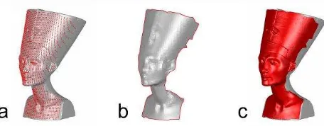
In this contribution a model of a statue, that is referred to as Nefertiti in the following, is used to demonstrate the proposed procedure that features an unsteady and rather complex surface. The input model is a scaled version of a digitised copy of the bust of Queen Nefertiti, New Kingdom, 18th dynasty ca. 1340 BCE, Egyptian Museum and Papyrus Collection, National Museums Berlin, Germany. Unauthorised external use of all figures in this manuscript is strictly prohibited. The model has a width of 1.95 m, a depth of 2.47 m and a height of 4.78 m. Figure 1 illustrates all required preparatory measures on the example of the introduced test model. Based on a single viewpoint a simulated point cloud is generated, represented by red points on the object’s surface (grey) as depicted in Figure 1 a. As laser scanners capture information in a quasi-laminar fashion yet describe surfaces, the simulated point clouds are converted into a surface representation by applying Delaunay-triangulation, as illustrated in Figure 1 b. These closed surface representations in form of meshes are then used to determine overlapping regions and the covered surface. As this process would be quite demanding in computational terms under usage of Boolean algebra, an alternative approach is proposed in this contribution. Therefore the boundaries of all meshes, represented by the red line in Figure 1 b, are projected onto copies of the original model surface, which is highlighted by the red coloured surface in Figure 1 c. Subsequently areas outside of the projected boundaries are deleted so that only the captured area from the current viewpoint remains. As a consequence the acquired surfaces from all viewpoints are transferred onto the model surface. Hence, overlapping regions can be determined quite easily as the geometric information is identical if overlap between two datasets exists.
Figure 1. Simulated point cloud (a), triangulated point cloud (b) and projection of the boundary onto the object of interest (c).
In order to achieve this all datasets have to be transferred into a common numbering system as every file contains its own system for vertices and triangles. It is obvious that the projected boundaries of all simulated scans onto a common geometry are very helpful in this context. The chosen file format for this sake is the obj-format (FILEFORMAT 2015) that is assembled by two basic lists. The first one contains all vertices in the file while the second one describes all triangles. An individual identifier helps to distinguish all vertices. Note that every file features its own numbering system so that equal triangles may be described by varying identifiers. Hence, a common numbering system has got to be created, that allows to identify redundant information respectively overlap. For this purpose, the vertices from all files are added to one list while redundant coordinate triples need to be removed, so that only unique entries result. These revised entries then receive novel identifiers after which the numbering of all triangles is updated. The procedure is demonstrated in Figure 2 on a simple example with two datasets. Figure 2 a and b show meshes that are both assembled of two triangles that feature four vertices. Triangle identifiers are highlighted by coloured numbers that are placed in the centre of each triangle while vertex identifiers are located in proximity to their corresponding vertex. It can easily be seen that the identifiers do not allow identifying common information namely the red triangle. After all datasets received superior identifiers for vertices and triangles the content of Figure 2 c emerges. If one now updates the identifiers of the meshes in the figure below based on the superior numbering system the following outcome arises:
Figure 2 a depicts triangles 2 and 3. Figure 2 b illustrates triangles 1 and 2.
Subsequently all triangles are added to a list which leads to 1, 2, 2, 3. As triangle 2 was listed twice it is describing an overlap between the two meshes. For computation of the associated surface the vertex identifiers for this triangle respectively their coordinates have to be retrieved.
Figure 2. Mesh 1 with according numbering (a), second mesh with own numbering of triangles and vertices (b). Combined
datasets with superior numbering (c)
3. ECONOMIC ASPECTS OF GEODETIC DATA ACQUISITION
A prerequisite before carrying out a classical engineering survey based on total station observations, is to perform a sophisticated network design respectively network optimisation. The major aim of this task is to receive an optimal solution that satisfies homogeneity of surveyed points in terms of accuracy and reliability, for instance by carefully controlling the redundancy numbers of observations. While these aspects are purely seen from an engineering perspective an economic point of view is also essential. For this sake a minimisation of the required expenditure of work on site needs to be undertaken which has to be smaller than a predefined value
A. This measure describes the maximum amount of time that is required to fulfil a defined The International Archives of the Photogrammetry, Remote Sensing and Spatial Information Sciences, Volume XLI-B5, 2016task in the field. It can either be defined by economic means or by a client for instance at a construction site where certain other design steps can only to be interrupted for a predefined amount of time during the survey. The following equation describes this problem by
A
a n
j j (1)where aj denotes the required effort for a single observation while nj represents the amount of repetitions. A detailed summary on network design is for instance given by GHILANI (2010 p. 455). While equation (1) is dependent to the required effort for a single observation and its repetitions within the context of total station surveys, this circumstance is now transferred for usage with TLS and follows
AVP HFOV, Res, Filter
. (2)This adaption of the original equation had to be made as the time of a single observation with a TLS can be conducted in split seconds. Concerning equation (2) it can be seen that the expenditure of work is a function of the required number of viewpoints VP as well as the current settings of the scanner and should be as large respectively smaller than the maximum expenditure of work
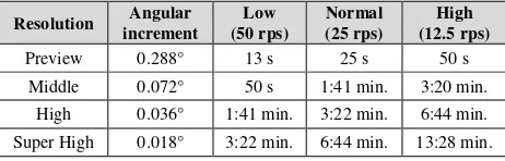
A. It has to be emphasised that the amount of viewpoints VP should be minimal due to the fact that changing the scanner’s position is the most time consuming part in comparison to the mentioned scanner settings. The settings of the scanner include the horizontal field of view HFOV, the chosen resolution Res and eventually filter frequency Filter where distance measurements can be repeated respectively filtered multiple times. In summary these settings influence the acquisition time carried out from one particular viewpoint. The horizontal field of view has been chosen in this context as it substantially influences the time of acquisition due to the fact that the revolution of the scan head around the rotation axis is significantly slower as the one of the deflection mirror.Table 1gathers the scanner performance of a Z+F Imager 5006 h (ZOLLER & FRÖHLICH 2010 p. 51, 82) in dependence to various scanner settings, as this device will be simulated in this contribution. The outer left column gathers several settings of the scanner that influences the angular increment (see second column from the left). The remaining columns contain information on different noise settings of the distance measurement unit. Each cell contains the according scan duration for a panorama scan. A comparative look at different scan settings reveals a large span of scan durations which hence directly influences the expenditure of work. As a consequence a setting has to be chosen by the user that requires the shortest length of stay on one viewpoint where the resolution is still sufficient not to cause unacceptable sampling errors. For the remainder of this subsection it is assumed that an appropriate setting has been chosen.
Table 1. Scanner performance of a Z+F Imager 5006h in dependence to various settings
Resolution Angular increment
Low (50 rps)
Normal (25 rps)
High (12.5 rps)
Preview 0.288° 13 s 25 s 50 s
Middle 0.072° 50 s 1:41 min. 3:20 min.
High 0.036° 1:41 min. 3:22 min. 6:44 min.
Super High 0.018° 3:22 min. 6:44 min. 13:28 min.
4. COMBINATORIAL VIEWPOINT PLANNING
This section describes the methodical procedure of the proposed combinatorial viewpoint planning algorithm. After a description of the basic algorithm several extensions will be introduced.
4.1 Description of the basic algorithm
Depending on a stated task different strategies may be applied for viewpoint planning, which hence requires different assessment procedures. This subsection will propose an economic strategy where the surface of a given object has to be captured to a certain degree. Therefore the variable completeness comp is introduced that serves as a quality measure respectively abort criterion of the planning algorithm. Hence comp can be interpreted as a threshold that specifies a required degree of completeness and is compared against a current set of cov that represents the surface area that is covered by one or several scans. As it is usually impossible to capture an object of interest entirely comp is chosen smaller than the sum of all surfaces cov which have been captured from different viewpoints without the according overlapping regions. Assuming that comp has been set as 0.9 the algorithm will try to find suitable viewpoints until the ratio between acquired and entire surface area lies above 90%. Furthermore the parameters
os [m²] and rO [%] are introduced that quantify the overlapping surface area respectively the percentaged overlapping area between two or more point clouds. The last mentioned parameter is described by the quotient between the entire area surface area ESA [m²] that is covered by two scans and the overlapping surface area os [m²] of the two point clouds.
100
os
rO
ESA
. (3)Now that all required parameters are introduced several desired aims should be defined for this economic planning strategy:
The number of viewpoints should be minimal:
VP
min
. Coverage cov should be at a maximum but at least larger than a preset boundary:
covmax with cov
comp.In the following a description of the proposed algorithm will be given on a simple example that is depicted in the left part of Figure 3. The outer grey shape depicts the area of interest aoi, while it can be seen that this area cannot be entirely covered by the given datasets A, B and C. The yellow area denotes the overlapping region between shape A and B while the orange form represents the overlap of contours B and C.
Figure 3. Example for computation of the proposed parameters (left) and flowchart of the basic algorithm (right) The International Archives of the Photogrammetry, Remote Sensing and Spatial Information Sciences, Volume XLI-B5, 2016
In order to satisfy the above mentioned criteria usage of a greedy algorithm as introduced before appears to be a suitable solution to the problem of finding an optimal set of TLS viewpoints. A downside of greedy algorithms is that they determine the solution in a sequential fashion which may be efficient from a computational point of view but not optimal. An optimal solution can only be found by considering all potential combinations of viewpoints.
As the algorithm should find the most economical solution, namely the smallest possible set of viewpoints VP, the initial value for VP is 1. Consequently for every viewpoint the acquired surface cov is computed and compared against the required level of completeness comp, as depicted in the flowchart on the right part of Figure 3. If this assumption does not hold, VP is increased by one and all combinations cmb are computed, A-B, A-C and B-C in this example. Subsequently all combinations are tested against the required level completeness
comp. If this requirement is not fulfilled VP is increased until all possible combinations have been considered. A downside of the combinatorial strategy is its growing complexity in dependence to an increasing amount of viewpoints. Based on the given example it is obvious that some combinations have to be considered as being irrational, for instance A-C, even if they fulfil all defined criteria. This statement can be justified by the lack of overlap between these datasets that consequently does not allow conducting registration of point clouds based on redundantly acquired areas. Hence, an extension is proposed in the following that only computes the acquired surface area and overlap if sufficient overlap is present. This action will drastically decrease the computational cost of the algorithm on one hand, on the other it rejects combinations that cannot be registered to a common dataset.
4.2 Consideration of sufficient overlap between viewpoints
In order to tackle the aforementioned issues an extension of the basic algorithm is proposed in the following, so that all point clouds have to overlap with at least one other dataset. Therefore all combinations of two datasets are established and tested for relative overlap rO [%]. This measure describes the ratio between sampled area and the according overlap. Subsequently all combinations are tested against a predefined threshold in order to check if sufficient overlap sO [%] is present. Now the question arises, how combinations that consist of more than two viewpoints can be tested for sufficient overlap without carrying the necessary computations.
A versatile tool for the representation of topological relations are so called incidence- and adjacency matrices, which have already been successfully been used to solve geodetic problems (LINKWITZ 1999). The last mentioned contribution uses topological procedures to reveal congruent point sets within a geodetic network. Therefore distances among points within the network are computed in all combinations, while only the ones are considered for further computations whose deviations to a previous epoch are within specified boundaries. Despite the fact that the given problem is different in terms of geometric properties of the input - sufficient overlap between meshes has to be determined in contrast to discrepancies of distances - a topological formulation can be achieved. This will be exemplified in the following based on the scenarios depicted in Figure 4.
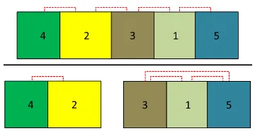
Figure 4. Cluster with continuous arrangement (top) and one of disconnected datasets (bottom)
The scenario on the top features five datasets that are arranged continuously where every point cloud is connected to its adjacent one (red dotted lines). This case will be referred to as scenario A in the following. The lower part of the figure, referred to as scenario B, depicts datasets that are divided into two clusters, despite the fact that also four connections are present. In order to assemble incidence matrix C all combinations of two datasets are established, while the resulting number defines the amount of rows of C. For the given example ten rows arise. The number of columns is specified by the amount of datasets, which are five in this case. Every cell that signifies a combination of viewpoints with sufficient overlap receives the entry 1 and is considered of being valid. Subsequently the adjacency matrix = T
C C Ccan be computed. Table 2 contains the adjacency matrix of scenario A in green as well as the one of scenario B in blue. An interesting piece of information is located on the diagonal of the matrix, which is highlighted in white, where the according number represents the amount of overlapping datasets. Dataset 1 of scenario A for instance is connected to datasets 3 and 5. Consequently the secondary diagonal contains information on which datasets are connected to each other. Now a procedure has to be found that is capable to identify if all datasets are connected among each other.
Table 2. Adjacency matrices for scenario A (green) and B (blue)
data 1 data 2 data 3 data 4 data 5
data 1 2 0 1 0 1
data 2 0 2 1 1 0
data 3 1 1 2 0 0
data 4 0 1 0 1 0
data 5 1 0 0 0 1
data 1 2 0 1 0 1
data 2 0 1 0 1 0
data 3 1 0 2 0 1
data 4 0 1 0 1 0
data 5 1 0 1 0 2
A comparison of the two matrices shows immediately that the values on the diagonal are equal even though the arrangement varies. The distribution of values is dependent to the topology as well as the definition of identifiers for individual files, hence the sole consideration of the diagonal is not a suitable measure for the identification of continuous point clouds. As a consequence other information from the adjacency matrix is used namely the secondary diagonal. The minimum requisite for the stated problem is that all point clouds are connected among each other at least once. For the identification process, which will be exemplified on the two scenarios depicted in Figure 4, all values that contain a valid connection are extracted. If one extracts all valid entries that are highlighted by 1 in the secondary diagonal, the following lists result:
Scenario A: 1-3, 1-5, 2-3 and 2-4, Scenario B: 1-3, 1-5, 2-4 and 3-5.
In order to identify if all datasets can be registered to a common one, a sequential method is proposed in the following, which will be demonstrated on scenario A at first. The procedure applies three lists that contain the following information:
Candidate list: Contains datasets to which associable viewpoints are added. At the start of the procedure this list contains one arbitrary combination of two viewpoints. It is replaced by the concatenation list if other viewpoints can be connected to one of the entries. Connection list: All valid connections that are
assembled by two viewpoints. This list decreases in length during the procedure.
Concatenation list: All viewpoints that describe a continuous arrangement. This list increases in size if other viewpoints can be associated to it.
For the given problem the length of the concatenation list has to be five. In order to check if this requirement holds, the first double of viewpoints is added to the candidate list that contains viewpoint 1 and 3. Subsequently the remaining viewpoints from the connection list are analysed if they contain at least one member from the candidate list. For the given case viewpoints 1-5 are connected to viewpoint 1 while viewpoints 2-3 are connected to viewpoint 3. As a consequence, the concatenation among viewpoints looks as follows where the current candidates are highlighted in green: 5-1-1-3-3-2. Note that the order of viewpoints has been arranged so that direct connections become immediately visible. Then this concatenation list is ordered leading to 1-1-2-3-3-5, while redundant entries are deleted. This list is now interpreted as the current candidate list that contains 1-2-3-5. Again the remainder of the connection list, that now only contains viewpoints 2-4 is analysed whether valid connections are given to one of the entries from the candidate list. As this is the case for viewpoint 2 the concatenation list follows 5-1-1-3-3-2-2-4 where the current members of the candidate list are again tinted in green. If one now reverses the order of the sequence and removes redundant entries the following list emerges: 4-2-3-1-5 – which is exactly the order in which the viewpoints are arranged in scenario A. After sorting the concatenation list and removal of repetitive entries the final candidate list appears that contains the following viewpoints 1-2-3-4-5. As the list contains five entries, which is equal to the amount of viewpoints that have to be connected among each other, the outcome has to be rated as valid.
Now the procedure is applied to scenario B. The first entry of the connection list is interpreted as the first pair of candidates containing viewpoints 1 and 3. Subsequently the connection list is queried for valid links which are viewpoints 1-5 and viewpoints 3-5. Hence the concatenation list contains 5-1-1-3 -3-5. It has to be pointed out that all viewpoints can be found twice in the list which means that all of them are connected to each other. After ordering and removing redundant entries the candidate list contains three entries namely 1-3-5. The only remaining entry in the connection list features viewpoints 2 and 4 which are not part of the candidate list. Hence there is no valid connection to the previously assembled cluster of three viewpoints. As the size of the candidate list is three and hence smaller than 5 this combination has to be rated as invalid so that no further calculations are conducted.
4.3 Consideration of sufficient surface topography
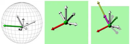
Even though the previously proposed extension of the original algorithm considers if sufficient overlap between point clouds is given, it does not analyse the surface topography in this region. The term surface topography denotes a sufficient distribution of spatial information within the overlapping area of two or more point clouds in all cardinal directions, that is required to carry out surface based registration. For clarification this circumstance should be exemplified in the following. It is assumed that two point clouds overlap by 90% yet the common region contains a planar surface. As a consequence the geometric information within the overlapping region is not sufficient to solve all degrees of freedom in 3D space within the context of a co-registration. Hence, an additional extension is proposed that computes numeric values which describe and characterise the geometric properties of the overlapping region among point clouds. A requirement onto this measure is that it has to be independent to the chosen coordinate system so that its numerical outcome solely expresses the characteristics of the local geometry. As a first step face normals of all triangles within the overlapping region need to be computed. As an outcome Cartesian coordinates arise that are converted into polar elements while only the directional components α and β are used. In order to assess the distribution of face normals a spherical grid is defined within a unit sphere that is bounded by equally sampled vectors that are all d degrees apart from each other. Then all polar components are sorted into the spherical grid while the according mean of all polar elements within a cell is computed. Furthermore the sum of entries within a cell is used as a measure for characterisation. This is achieved by interpreting the sum of entries within a cell as the length of a vector while the directional components are defined by the mean polar elements of the according element. Then the cell with the most entries is determined which is referred to as the most dominant direction (MDD). In other words the MDD expresses in which direction most of the face normals within the region of overlap are oriented. In addition this strategy achieves the desired independence against the choice of a coordinate system. After the MDD has been computed all entries within the spherical grid are normalised. The left part ofFigure 5 shows the spherical grid with the normal vectors of the overlapping region. The largest entry is highlighted in green.
Figure 5. Spherical grid with normal vectors (left). The green vector depicts the most dominant direction in the centre of the
figure. The red vector denotes the SDD on the right.
Based on the desired distribution of face normals all remaining normal vectors are set into relation to the MDD. Therefore a plane is computed whose normal vector is described by the MDD and starts in the origin of the coordinate system. Subsequently all normal vectors are projected onto this plane while the largest entry is determined which will be referred to as second dominant direction (SDD). As MDD and SDD are perpendicular to each other and because all normal vectors have The International Archives of the Photogrammetry, Remote Sensing and Spatial Information Sciences, Volume XLI-B5, 2016
been normalised this procedure assesses the relation between the two vectors. A view that is aligned parallel to the MDD is depicted in the centre of Figure 5while the resulting SDD is coloured in red. At last a vector is computed by the cross product of the MDD and SDD, as depicted in the right part of Figure 5, to which all normal vectors are projected. Note that the resulting vector highlighted in yellow has been increased in length for demonstrative purposes only. Analogous to the other dominant directions the largest projected vector is determined which is referred to as the third dominant direction (TDD) and is coloured in pink. The desired relation among all dominant directions should be MDD = 1, SDD = 1 and TDD = 1 which would mean that they are all perpendicular to each other. Hence the proposed procedure allows to numerically assess the geometrical characteristics of an overlapping region. The previously mentioned scenario consisting solely of two perpendicular planes would lead to quality measures of MDD = 1, SDD = 1 and TDD = 0. As a consequence the geometrical content of the overlapping region has to be rated as insufficient for surface based registration. In the following the procedure is demonstrated on the overlapping region between viewpoint 1 and 2 as illustrated in Figure 6. The red dataset has been acquired from viewpoint two while the dark grey mesh was observed from viewpoint 1. After computing the overlapping region, which spans over 6.19 m², between these two triangular meshes the light grey bust emerges. It can be seen that the boundaries of the overlapping region can be found in this resulting dataset e.g. the characteristic shape of the right boundary from viewpoint 2. In addition the resulting maximum geometric contrast is illustrated by three colour coded vectors. The MDD amounts per definition to 100% while the SDD represents 54.4% and the TDD measures slim 2.51%.
Figure 6. Datasets acquired from viewpoint 2 (red) and viewpoint 1 (dark grey). The overlapping region of these two
meshes, as depicted in the centre, is coloured in light grey.
5. APPLICATION OF THE ALGORITHM
The capability of the approach in demonstrated on a scenario with ten viewpoints has been created which have been circularly sampled around the dataset with a radius of 20 m. It has to be mentioned that the way of how potential viewpoints are defined depends on the object of interest. A common strategy in the context of buildings for instance is to form a grid. Note that in this article a limited number of viewpoints are considered for illustrative reasons. However, the proposed methodology is capable to solve more complex problems yet with significantly higher computational costs. The angular resolution has been set to 0.18 , so that approximately four million vectors that simulated observations by a laser scanner from each viewpoint resulted. All viewpoints were located about 1.6 m above the lowest point of the bust. The surface of interest measures 29.94 m² and covers the bust without the top part of the helmet as this region is not visible from any viewpoint. A summary on the data acquired from all simulated viewpoints is given in Table 3.
Table 3. Overview of the simulated viewpoints
1 dk. grey
2 red
3 orange
4 lt. green
5 cyan
A [m²] 11.04 11.28 10.52 11.36 10.45
Δ A [%] 36.87 37.67 35.13 37.94 34.90
HFOV [°] 17.19 17.46 21.84 22.71 23.20
6 pink
7 yellow
8 dk. green
9 blue
10 purple
A [m²] 11.02 12.22 11.56 12.17 10.63
Δ A [%] 36.81 40.81 38.61 40.65 35.50
HFOV [°] 18.38 18.98 23.27 22.03 21.26
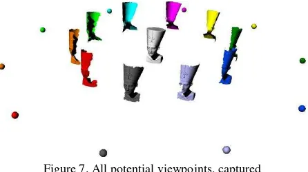
Note that the colours mentioned in the first row are used for colour coding in the following illustrations. The first and fifth rows denote all viewpoints VP, while the rows marked by A gathers the acquired area. The relation between the entire surface of the bust and acquired area from single viewpoints can be found in rows labelled with Δ A. The horizontal field of view HFOV can be found in rows four and eight and denote the horizontal angle that encloses the object of interest from a certain viewpoint. Figure 7 illustrates all possible viewpoints (spheres) and acquired surfaces (mesh segments) shaded according to the above mentioned colour code. The input model is coloured in light grey and located in the centre of the scene.
Figure 7. All potential viewpoints, captured surfaces and original model of interest.
For the first example a combination of viewpoints with a level of completeness comp of at least 95% should be detected by the algorithm described under subsection 4.1. The computation time was 404 s by using a 3.07 GHz quad core processor with 12 GB of RAM. In total 165 combinations and the ten viewpoints have been checked, while a solution consisting of three viewpoints, namely 2 (red), 5 (cyan) and 9 (blue) as depicted in Figure 8, was found covering 96.21% of the model’s surface. The overlap between all viewpoints sums up to 29.54% in relation to the entire surface.
Figure 8. Outcome of the algorithm for a level of completeness of at least 95% The International Archives of the Photogrammetry, Remote Sensing and Spatial Information Sciences, Volume XLI-B5, 2016
In order to demonstrate the increasing computational demand for a growing number of combinations the desired ratio of coverage has been set to 99%. The computation time slowed down enormously to 5509 s while 837 combinations of different viewpoints have been tested. A coverage of 99.12% was found for viewpoints 2, 3, 5, 7, 8 and 9. The overlap between the meshes sums up to 92.92%. Hence it is obvious that additional criteria have to be introduced that reduce the amount of possible combinations. The previous implementation opted to find a combination where the number of viewpoints was at a minimum while the coverage should be possibly large. As a consequence the overlap between adjacent point clouds was fairly small that eventually does not allow carrying out surface based registration and hence makes it impossible to create a continuous 3D-model of the object of interest.
By deploying the first extended algorithm, which has been introduced in subsection 4.2, the given test case is now processed with the following settings:
Completeness comp of at least 90%. Relative overlap rO of at least 10%.
From 45 combinations that consisted of two point clouds 29 (64%) satisfied the stated criterion for sufficient overlap. After 287 seconds a valid solution, namely 2-3-6-9, has been found assembled by viewpoints that feature a level of completeness of 93.06%. The adjacency matrix looks as follows:
2 1 0 1
1 2 1 0
0 1 2 1
1 0 1 2
Hence each viewpoint has got two connections. Figure 9 illustrates the result generated by the extended algorithm.
Figure 9. Outcome of the algorithm for a level of completeness of at least 90% with consideration of sufficient overlap
In order to demonstrate the increased performance of the algorithm the required level of completeness was set to 95% with a minimum overlap of 30%. The result has been computed in 321 seconds and is assembled by six viewpoints (3-4-5-8-9-10). The computation of a solution with the mentioned settings containing all viewpoints took 392.26 seconds for which 127 combinations were analysed. The naive computation without considering sufficient overlap required to analyse 1013 combinations in total of which four combinations fulfilled the level of completeness criterion of 95%. On average the analysis of one combination took about 6.57 seconds so that 6658 seconds of computation were required. Another option to decrease the computational cost is to define an upper margin respectively a range of overlap.
Another test has been conducted based on the final extended algorithm from section 4.3 where the following settings were defined:
Completeness comp of at least 95%. Relative overlap rO of at least 10%.
The geometric contrast has to satisfy at least the following requirements:
MDD = 100%, SDD, = 10% and TDD = 1%.
Division of a normal sphere into 24 horizontal and vertical sectors.
It has to be mentioned that the bandwidth of normal directions for each simulated viewpoint of this dataset never exceeds 180° as a closed object with a convex characteristic is acquired. If for instance the interior of a building has been captured the potential bandwidth of normals increases to 360°. Hence the ratio of MDD, SDD and TDD may be more favourable than in this example. Table 4 gathers an excerpt from all combinations that are assembled of two viewpoints. In this case only adjacent viewpoints are exemplarily listed where rows one and seven depict the current combination. Rows marked by MDD, SDD and TDD contain the corresponding values in percent. It can be seen that the surface topography appears to be weak in most cases apart from the overlapping region between viewpoint 6 and 7. The last two rows contain information about the extent of the overlapping region in percent as well as the entire covered surface in m².
Table 4. Overview of adjacent viewpoints in terms of overlap and geometric contrast
Combination /
Parameter 1-2 2-3 3-4 4-5 5-6
MDD [%] 100 100 100 100 100
SDD [%] 65.22 54.62 43.15 43.42 53.17
TDD [%] 2.51 1.65 0.01 0.05 15.23
Overlap [%] 42.89 53.01 53.16 63.92 58.62
Covered surface [m²] 14.43 14.05 14.44 14.19 13.82
Combination /
Parameter 6-7 7-8 8-9 9-10 1-10
MDD [%] 100 100 100 100 100
SDD [%] 71.91 42.27 40.58 79.09 51.55
TDD [%] 13.32 13.38 0.03 0.01 0.13
Overlap [%] 55.67 65.51 56.03 66.73 57.09
Covered surface [m²] 13.57 13.61 14.5 13.31 13.8
A solution with the aforementioned settings has been found after 169.16 seconds which is depicted in Figure 10. In total a coverage of 95.13% has been computed for which six viewpoints, namely 2-3-6-7-8-10, would have to be observed.
Figure 10. Outcome of the algorithm that considers sufficient overlap and surface topography The International Archives of the Photogrammetry, Remote Sensing and Spatial Information Sciences, Volume XLI-B5, 2016
6. ESTIMATION OF THE EXPENDITURE OF WORK
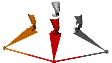
After several variants of the original algorithm have been proposed the expenditure of work is computed. For this purpose it is assumed that one operator is capable to carry a tripod as well as a stand-alone scanner at 1.5 m/s respectively 5.4 km/h. The distance that the operator has to carry the scanner and other required equipment is defined by the direct connection between chosen viewpoints as long as they do not intersect the object. It is assumed that it takes 120 seconds per viewpoint to set up the sensor and another 60 seconds that the scanner requires for initialisation and acquisition of a pre-scan. The setting for data acquisition has been defined as “middle”, as listed in Table 1, while a panorama-scan takes 101 seconds. In order to determine the time that is required for scanning the last column of Table 5 is used in which the horizontal field of view for every viewpoint is listed. For every solution the sum of all HFOV’s is computed that is then set into relation with the time that is needed to capture a panorama scan. For explanatory reasons a simple example will be given in the following where data from viewpoints 1, 2 and 3 are captured. Figure 11 illustrates the scenario where all related elements are coloured in accordance to the viewpoint’s tones: viewpoint 1 (dark grey), viewpoint 2 (red) and viewpoint 3 (orange). The circular segments originating from the viewpoints (spheres) depict the horizontal field of view that sum up to 17.19° for viewpoint 1, 17.46° for viewpoint 2 and 21.84° for viewpoint 3. The cylindrical connections among viewpoints denote the path that an operator has to travel in order to capture the scenario.
Figure 11. Acquired data from viewpoints 1 (grey), 2 (red) and 3 (orange) with object of interest in the background
In total 56.49° have to be scanned in horizontal direction so that the acquisition time will take (56.49°/180°)∙101 s = 31.7 s. As data will be captured from three viewpoints preparation of the scanner will take 3∙120 s = 360 s while the initialisation phase of the scanner adds up to 3·60 s = 180 s. For consideration of the time of transportation the distance between viewpoints of 27.72 m is assumed. As mentioned earlier a speed of 1.5 m/s is expected so that this task will take (27.72 m/1.5 m/s) = 18.5 s. In total, the expenditure of work adds up to 31.7 s + 360 s + 180 s + 18.5 s = 590.2 s. A comparison of the expenditure of work for several scenarios is given in Table 5. It can be seen that the EOW is mainly depends on the number of viewpoints n.
Table 5. Comparison of the computed results
comp [%]
| rO [%]
∑ HFOV
[°]
cov
[%] n d [m] cmb
EOW [s]
95 | 0 62.69 96.21 3 70.4 165 622
99 | 0 126.78 99.12 6 84.1 837 1207
95 | 10 134.31 96.84 6 81.8 127 1210
max | min 206.32 98.52 10 111.3 1013 818
7. CONCLUSIONS AND OUTLOOK
A combinatorial viewpoint planning algorithm has been proposed based on a given 3D-model. Besides a basic implementation geometric restrictions can be defined that yield to a certain overlap among simulated point clouds for the sake of surface based registration. The introduction of a measure for the surface topography ensures that the overlapping region of two point clouds is suitable for registration. Based on several computed viewpoint plans the required expenditure of work is estimated, that it would take to capture a scene in the field, which is vital for the preparation of field trips, expeditions or other survey campaigns. Future work will focus on improving the method featured in section 4.3 that describes the surface topography of the overlapping region. Furthermore the problem has to be tackled how viewpoint plans can be transformed into the object space when carrying out the actual measurements.
REFERENCES
Ahn, J.,Wohn, K., 2015. Interactive scan planning for heritage recording. Multimedia Tools and Applications, Springer publishing, p.1-21.
Appel, A., 1968. Some techniques for shading machine renderings of solids. In: Proceedings of the spring joint computer conference, New York, USA, p. 37-45.
Chvatal, V., 1979. A greedy heuristic for the set-covering problem. Mathematics of operations research, 4, p. 233-235.
Fileformat, 2015. Wavefront OBJ File Format Summary. http://www.fileformat.info/format/wavefrontobj/egff.htm (accessed 09.12.2015).
Ghilani, C. D., 2010. Adjustment computations: spatial data analysis. John Wiley & Sons.
Karp, R. M., 1972. Reducibility among combinatorial problems. Springer US, p. 85-103.
Linkwitz, K., 1999. About the generalised analysis of network-type entities. In: Quo vadis geodesia ... ? University Stuttgart, Report Nr. 199.6, p. 279-293.
Luhmann, T., Robson, S., Kyle, S., Harley, I., 2011. Close range photogrammetry: Principles, methods and applications, Whittles publishing, p. 1-531.
Scott, W., Roth, G., Rivest, J. F., 2003. View planning for automated 3D object reconstruction inspection. ACM Computing Surveys, 35(1).
Slavik, P., 1996. A tight analysis of the greedy algorithm for set cover. In: Proceedings of the twenty-eighth annual ACM symposium on theory of computing, p. 435-441.
Soudarissanane, S., Lindenbergh, R., 2011. Optimizing terrestrial laser scanning measurement set-up. In: ISPRS Laser Scanning 2011, Calgary, Vol. XXXVIII, p. 1-6.
Zoller & Fröhlich, 2010. Z+F Imager 5006 h Owner’s Manual. The International Archives of the Photogrammetry, Remote Sensing and Spatial Information Sciences, Volume XLI-B5, 2016