ACCELERATION OF SEA LEVEL RISE OVER MALAYSIAN SEAS FROM SATELLITE ALTIMETER
A I A Hamida*, A H M Dinab*, N F Khalida, K M Omara,
a Geomatic Innovation Research Group (GIG), Faculty of Geoinformation and Real Estate, Universiti Teknologi Malaysia, 81310 Johor Bahru, Johor, Malaysia.
b Geoscience and Digital Earth Centre (INSTEG), Universiti Teknologi Malaysia, 81310 Johor Bahru, Johor, Malaysia. *[email protected]
KEY WORDS: Climate Change, Sea Level Rise, Satellite Altimeter
ABSTRACT:
Sea level rise becomes our concern nowadays as a result of variously contribution of climate change that cause by the anthropogenic effects. Global sea levels have been rising through the past century and are projected to rise at an accelerated rate throughout the 21st century. Due to this change, sea level is now constantly rising and eventually will threaten many low-lying and unprotected coastal areas in many ways. This paper is proposing a significant effort to quantify the sea level trend over Malaysian seas based on the combination of multi-mission satellite altimeters over a period of 23 years. Eight altimeter missions are used to derive the absolute sea level from Radar Altimeter Database System (RADS). Data verification is then carried out to verify the satellite derived sea level rise data with tidal data. Eight selected tide gauge stations from Peninsular Malaysia, Sabah and Sarawak are chosen for this data verification. The pattern and correlation of both measurements of sea level anomalies (SLA) are evaluated over the same period in each area in order to produce comparable results. Afterwards, the time series of the sea level trend is quantified using robust fit regression analysis. The findings clearly show that the absolute sea level trend is rising and varying over the Malaysian seas with the rate of sea level varies and gradually increase from east to west of Malaysia. Highly confident and correlation level of the 23 years measurement data with an astonishing root mean square difference permits the absolute sea level trend of the Malaysian seas has raised at the rate 3.14 ± 0.12 mm yr-1 to 4.81 ± 0.15 mm yr-1 for the chosen sub-areas, with an overall mean of 4.09 ± 0.12 mm yr-1. This study hopefully offers a beneficial sea level information to be applied in a wide range of related environmental and climatology issue such as flood and global warming.
1. RESEARCH BACKGROUND
Global sea levels have been rising through the past century and are projected to rise at an accelerated rate throughout the 21st century (IPCC, 2014). This has motivated a number of authors to search for already existing accelerations in observations, which would be, if present, vital for coastal protection planning purposes. AVISO’s Sea Level Research Team conducts a study to investigate the Global Mean Sea level (GMSL) since January 1993 to December 2015, and it shows that GSMSL has increased to a rate of 3.37 mm year-1 (AVISO, 2016). The major contributions to 20th and 21st century sea level rise are thought to be a result of ocean thermal expansion and the melting of glaciers and ice caps (Church et al., 2008).
Acceleration of sea level rise between the periods 1993 to 2009 when satellite measurements are available and in-situ data from tide gauges displayed the rate of 2.8 ± 0.8 mm yr-1 (Church and White, 2011), whilst altimetry suggested a consistent rate of 3.3 ± 0.4 mm yr-1 for a similar period 1993-2010 was recently revealed by Hay et al. (2015). Sea level rise due to climate change is non-uniform globally, thus necessitating regional estimates.
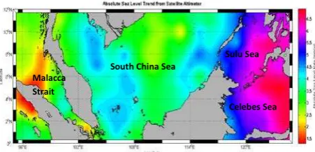
The Southeast Asian region is exemplified by its unique geographical settings (Din, 2014). Geographically, Malaysia is surrounded by water: the South China Sea, the Malacca Strait, the Sulu and Celebes Sea that are surrounded by a large population inhabits low lands in coastal areas while bound by two major oceans, the Pacific and Indian oceans. Figure 1
demonstrates the absolute sea level trend over Malaysian seas and the results clearly indicate that the absolute sea level trend is ascending and varying from place to place over the seas.
Figure 1. Map of absolute sea level trend over Malaysian seas. Units are in mm yr-1 (Din, 2014)
The rate of sea level varies and gradually increases from east to west of Malaysia (Din, 2014). The analysis of regional sea level rate over the Malaysian seas from multi-mission satellite altimetry has been conducted previously by Din (2014), with regard to the different techniques and various processing methods presented in this extensive study, the sea level trend for Malaysia region fulfilled that it has been rising with an overall mean of 4.47 ± 0.71 mm yr-1 based on altimeter and vertical-corrected tidal data. Meanwhile the sea level rate of Malaysian seas based on the altimetry data solely is 4.56 ± 0.68 mm yr-1. With the advancement of new technology, the data acquisition of sea level should be improved. As tide gauges are attached to
Malacca Strait
Sulu Sea
land and only found in coastal area, an alternative method has been used to acquire sea level data in order to overcome the uneven geographical distributions of tide gauge stations installed in coastal areas and there is no long term records for deep ocean (Azhari, 2003; Din, 2014; PSMSL, 2016). By measuring the absolute sea level from space, i.e. satellite altimeter technique, the deep ocean can be covered hence compliments the deficiency on the traditional coastal tide gauge instruments for monitoring sea level change over Malaysian seas, particularly for deep ocean.
This paper is aimed to quantify the sea level trend over Malaysian Seas in recent years, which is based on a combination of multi-mission satellite altimeters over a time span of 23 years, starting from January 1993 to December 2015. It covers the entire Malaysian seas, namely, Malacca Straits, South China Sea, Celebes Sea and Sulu Sea. Eight altimeter missions, i.e. TOPEX, Jason-1, Jason-2, ERS-1, ERS-2, Envisat, Cryosat-2 and Saral were used to get the absolute sea level from the Radar Altimeter Database System (RADS). Subsequently, the satellite derived sea level data is verified with the sea tidal data. Though the principle of satellite altimeter is based on the straightforward fact that a period of time is equivalent to the distance, the approach of bearing a sea level profiles is far more complex in practice.
Principle of Satellite Altimeter
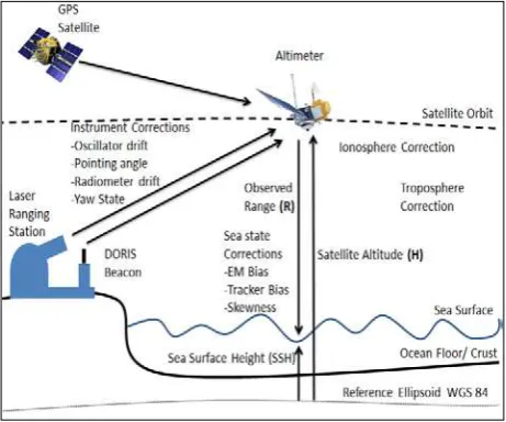
The distance between the satellite and the sea surface is measured from the round-trip travel time of microwave pulses emitted downward by the satellite radar, reflected back from the ocean, and received again on board. Figure 2 illustrates the diagram of satellite altimeter system and its principle.
Figure 2. Schematic view of satellite altimeter measurement (modified after Watson, 2005; Din, 2014)
Independent tracking systems are used to compute the satellite’s three-dimensional position relative to an earth-fixed coordinate system. Profiles of sea surface height, or sea level, with respect to a reference ellipsoid is obtained by combining these two measurements (Din, 2014). Sea level obtained or sea level anomaly (SLA) derived is used to compute the sea level trend.
Nevertheless, several factors must be taken care that ensuring the data acquired is precisely such as, atmospheric corrections
(i.e., ionosphere and troposphere), geophysical corrections (i.e., tides, geoid/ mean sea surface, sea state bias and inverse barometer), reference systems, precise orbit determination, varied satellite characteristics, instrument design, calibration, and validation (Naeije et al., 2008).
By adopting a similar concept from Fu and Cazenave (2001), the corrected range Robs as:
(1)
Where,
Robs = c t/2 is the computed range from the travel time, t
observed by the on-board ultra-stable oscillator (USO), and c is the speed of the radar pulse neglecting refraction (approximate 3 x 10⁸ m/s)
∆Rdry : Dry tropospheric correction
∆Rwet : Wet tropospheric correction
∆Riono : Ionospheric correction
∆Rssb : Sea-state bias correction
The corrected range is then converted to the sea surface height, h relative to the reference ellipsoid given as (Fu and Cazanave, 2001):
(2)
Where,
H : The height of the mass centre of the spacecraft above the reference ellipsoid, estimated through orbit determination
The actual sea surface height, h obtained is not sufficient for oceanographic applications because it is a superposition of geophysical signals. In order to remove the external geophysical signals from the sea surface height, Equation (3) is applied (Fu and Cazenave, 2001). It is noted that these are corrections for geophysical effects, but they behave like range corrections.
(3)
Where,
hD : Dynamicsea surface height
hgeoid : Geoid correction
htides : Tides correction (ocean tide, load tide, pole
tide, solid earth tide)
hatm : Dynamic atmospheric correction
The following steps are to merge the range and geophysical corrections into a complete set of altimeter corrections. By merging the range and geophysical corrections, the dynamic sea surface height, hD, is obtained from the height, H, of the
spacecraft, and the range, Robs. The equation is written as (Fu and Cazenave, 2001):
hD = H - Robs - ∆hdry - ∆hwet - ∆hiono - ∆hssb - hgeoid - htides - hat (4)
Ordinarily, for sea surface height variation studies, it is more appropriate to refer the sea surface height to the mean sea surface (MSS) rather than to the geoid surface, thus forming the SLA, hsla, written as (Fu and Cazenave, 2001):
By subtracting the MSS, it removes the dynamic sea surface height temporal mean variations and forms SLA that, in principle, have zero mean. This is due to the fact that the MSS is usually calculated by averaging altimetric observations over a long period of time and combining data from several satellite altimeter missions. When eliminating the temporal mean, the temporal mean of the corrections is eliminated and only the time variable component of the corrections is then a concern.
2. RESEARCH APPROACH 2.1 Research Area Identification and Data Processing The primary area of interest covers Malaysian seas, namely, Malacca Straits, South China Sea, Celebes Sea and Sulu Sea. It
ranges between 0° N ≤ Latitude ≤ 14° N and 95° E ≤ Longitude ≤ 126° E comprising the entire Malaysia region. Within the time
span of 23 years, from January 1993 to December 2015 consecutively, the sea level trend is quantified from SLA data obtained from the multi-satellite altimeter. RADS meanwhile, presents as processing software for altimeter data processing and provides user to able to define the most suitable corrections to be applied to the data. Beforehand, data verification is performed between altimetry data with selected tidal data in order to produce comparable results.
2.2 Tidal Data
The monthly sea level data for data verification in the domain of interest were acquired from The Permanent Service for Mean Sea Level (PSMSL) data bank. The comparison of sea level from altimetry and tidal data has been carried out by extracting monthly SLA average at the tide gauge locations and the altimeter track that are nearby the tide gauge stations. The pattern and correlation of sea level anomalies of both measurements are evaluated over the same period in each area. From Figure 3, the selected tide gauges are positioned along the east coast of Peninsular Malaysia, namely Geting, Cendering, Tg. Gelang, P. Tioman and Tg. Sedili while Sabah and Sarawak consist of Bintulu, Labuan and K. Kinabalu. All of these tide gauge stations face the South China Sea due to it is an open sea, therefore more satellite tracks can be acquired.
Figure 3. The distribution of tide gauge stations that was employed in data verification
2.3 Multi-mission Altimetry Data and Processing
Eight (8) satellite altimeter missions are involved in this study: TOPEX, Jason-1, Jason-2, ERS-1, ERS-2, EnviSat, Cryosat-2 and Saral to extract SLA data. The time period of altimetry data is covered from January 1993 to December 2015 Details regarding the altimetry data used in this study are described in Table 1:
RADS presents as processing software for altimeter data processing and provides user to able to define the most suitable corrections to be applied to the data (Din, 2014).
Table 1. Altimetry data selected for data verification
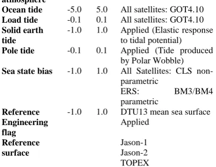
Figure 4 shows the overview of altimetry data processing in RADS. The sea level data are corrected for orbital altitude; altimeter range corrected for instrument, sea state bias, ionospheric delay, dry and wet tropospheric corrections, solid earth and ocean tides, ocean tide loading, pole tide electromagnetic bias and inverse barometer corrections as displayed by the Equation 5. The bias is reduced by applying specific models for each satellite altimeter mission in RADS as shown in Table 2.
Figure 4. Overview of altimetry data processing in RADS (Din, 2014)
Table 2. Corrections and models applied to RADS altimeter processing
-0.6 0.0 All satellites: Radiometer measurement
Ionosphere -0.4 0.04 All satellites: Smoothed dual-frequency,
ERS: NIC09
Dynamic -1.0 1.0 All satellites: MOG2D
Satellite Phase Sponsor Period Cycle
atmosphere
Ocean tide -5.0 5.0 All satellites: GOT4.10 Load tide -0.1 0.1 All satellites: GOT4.10 Solid earth
tide
-1.0 1.0 Applied (Elastic response to tidal potential)
Due to factors such as orbital errors and the discrepancy of the satellite’s orbit frame, the sea surface heights (SSH) from different satellite missions need to be adjusted to a “standard” surface. The minimization was achieved with the orbit of the NASA-class satellites held fixed and those of the ESA-Class satellites adjusted simultaneously given that NASA-class satellites surpasses the accuracy of the orbits and measurements of the ESA-class satellites (Trisirisatayawong et al., 2011; Din, 2014; CACRS, 2015). A distance-weighted gridding was applied in order to lose as little information as possible while still obtaining meaningful values for grid points located between tracks. The use weighting function is to establish the points close to the centre to be important and points far from the centre to be relatively insignificant. The weighting function is based on the Gaussian distribution (Singh et al., 2004, Din, 2014).
(6)
Where, the sigma, σ represents the weight assigned to a value at a normal point located at a distance r from the grid point. Then the daily data from multi-mission satellite altimeter are then filtered and gridded to sea level anomaly bins using Gaussian weighting function with sigma 2.0. The daily solutions for sea level anomalies are then combined with the monthly average solutions. This step is done in order to standardize the final monthly altimeter solution with the monthly tide gauge solution while improves the correlation between monthly solutions of altimetry and tidal data since the satellite altimeter flies over the tide gauge only three times in a month for the best case scenario (Din, 2010).
2.4 Analysis of Sea Level using the Robust Fit Technique Robust fit analysis is a standard statistical technique that concurrently deals with solution determination and outliers
detection. In this robust fit approach, a linear trend is fitted to
the annual sea level time series in an Iteratively Re-weighted Least Squares (IRLS) technique (Holland and Welsch, 1977; Din, 2014). Depending on the deviations from the trend line, weights of measurements are adjusted accordingly. The trend line is then re-fitted. The process is repeated until the solution converges. The weights of the observations (wi) are readjusted
by the adopted bi-square weight function, whose relationship with normalized residuals, (ui) can be written as (Holland and
Welsch, 1977; Din, 2014):
wi = (7)
Where,
ui =
ri : Residuals,
hi : Leverage,
S : Mean absolute deviation divided by a factor 0.6745 to make it an unbiased estimator of standard deviation
K : A tuning constant whose default value of
4.685 provides for 95% asymptotic efficiency
as the ordinary least squares assuming a Gaussian distribution
Observations that are assigned a zero weight in any iteration are declared as outliers and eliminated from further computation (Holland and Welsch, 1977; Din, 2014).
3. RESULTS AND DISCUSSIONS 3.1 Data Verification: Altimeter versus Tide Gauge
The SLA data that will be benchmarked from both sources is focused on the pattern and the correlation analysis. Altimetry data which are derived from RADS needs to be verified before performing trend analysis. Eight (8) tide gauge data have been selected fronting the South China Sea. Data verification is accomplished by extracting the monthly SLA average at the tide gauge location and the altimeter track that are nearby the tide gauge station. The pattern and correlation of both measurements are evaluated over the same period in each area in order to produce comparable results, starting from 1st January 1993 to 31st December 2015.
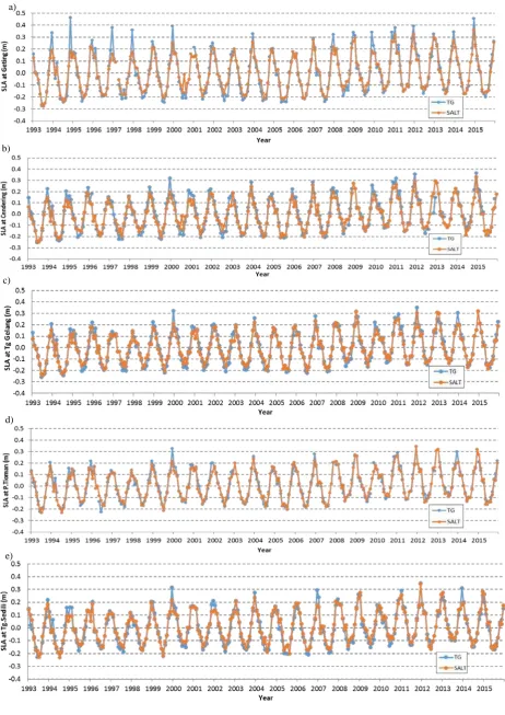
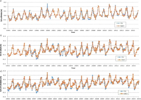
The time series patterns of altimetry data and tidal data that are displayed in Figure 5 is for the Peninsular Malaysia tide gauge stations while Figure 7 is the pattern in Sabah and Sarawak tide gauge stations. All the graphs show the similarity in the pattern of sea level from altimeter and tide gauge indicates good agreements for all stations accordingly. However, there is a fallen in sea level in the late 2015 to the year 2016. This may due to a strong impact of El Niño that happen in the year 2015 recently. The effect of La Niña can be seen in the graph during year 1999 until 2000.
All tidal data achieve an astonishing root mean square (RMS) difference when compare to altimetry data that range from 0.0260 m to 0.0475 m. The highest RMS obtained is from Geting tide gauge station, which is 0.0475 m, whereas, Labuan tide gauge station got the lowest RMS difference (0.0260 m). The correlation analysis for all location produces confidence result with the R2 value that range between 0.8401 to 0.9413 as shown in Figure 6 and 8. The summary of R2 and RMS difference at each station is displayed in Table 3.
Table 3. R2 and RMS difference value
Stations R2 RMS difference
Geting 0.9413 0.0475
Cendering 0.9243 0.0459
Tg. Gelang 0.9380 0.0379
Figure 5. Sea level comparison between altimetry and tidal data at the Geting (a), Cendering (b), Tg. Gelang (c), P. Tioman (d), Tg Sedili (e), of Peninsular Malaysia.
a)
b)
c)
d)
Figure 6. The altimetry and tidal sea level correlation analysis at the Geting (a), Cendering (b), Tg. Gelang (c), P. Tioman (d) and Tg. Sedili (e)
Figure 7. Sea level comparison between altimetry and tidal data at the Bintulu (a), Labuan (b), K. Kinabalu (c) of Sabah and Sarawak a)
d)
a)
b)
c)
Cendering
R2 = 0.9243
RMSE = 0.0459 m
b) c)
e)
Tg Gelang
R2 = 0.9380
RMSE = 0.0379 m
P. Tioman
R2 = 0.9404
RMSE = 0.0322 m
Tg Sedili
R2 = 0.9270
RMSE = 0.0379 m Geting
R2 = 0.9413
Figure 8. The altimetry and tidal sea level correlation analysis at the Bintulu (a), Labuan (b) and K. Kinabalu (c)
3.2 Sample of Robust Fit Data
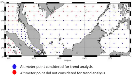
As mentioned in Section 2.2, the Robust Fit Technique has been utilized in order to interpret the absolute sea level trend. Then, the Malaysian seas i.e Malacca Straits, South China Sea, Celebes Sea and Sulu Sea, is mapped based on the numbers of altimeter-derived level anomaly points that are extracted as portrayed in the Figure 10.
Figure 9. The locations of the absolute sea level trends extracted for further analysis
Referring to Figure 9, the blue dots signify the altimeter points that are deliberate for computing the absolute sea level trend analysis for the Malaysian seas. The blue dots are considered to be within the Malaysian seas, which is the main area of concern in this study. In the meantime the red dots are only used for
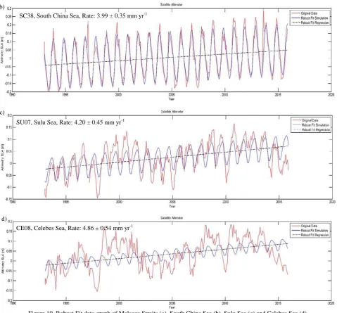
trend representation in those areas, as it is not the main focus areas. Figure 10 represents the example of the Robust Fit data graph of Malacca, South China Sea, Sulu Sea and the Celebes Sea.
Irregular pattern also noticeably in the Figure 10 (a) as tides or water flows mainly enters from side of the strait and then influenced by the geometrical changes from the northwest to southeast and the tiny islands at the southeast end (Akdag, 1996).
The effects of El Niño and La Niña clearly shows in the Malacca Straits as demonstrated in Figure 11 (a), where sea level drops below normal values late 1997 (El Niño), goes back to normal mid-1998, and overshoots a little at the end of 1998 (La Niña). Though the South China Sea did not effect from these events, The Sulu Sea and Celebes Sea graph also indicates the effect of El-Niño and La-Niña in those years. This due to the Sulu and Celebes seas is a semi-closed sea
In the late 2015, El Niño once again hit the Malaysia region. It is visible in the Figure 10 when a sudden drop at the late 2015 occur at almost Malaysian seas. This condition will affect the sea level on this region where the sea level will decrease compared to the previous sea level. Hence, in the case of Malaysian Seas, the closed and semi-closed seas may reflect the effects of El Niño and La Niña events.
Bintulu
R2 = 0.8375
RMSE = 0.0319 m
Altimeter point did not considered for trend analysis Altimeter point considered for trend analysis
Labuan
R2 = 0.9071
RMSE = 0.0260 m
K. Kinabalu
R2 = 0.9069
RMSE = 0.0299 m
MA16, Malacca Straits, Rate: 2.54 ± 0.55 mm yr-1
a) b) c)
Figure 10. Robust Fit data graph of Malacca Straits (a), South China Sea (b), Sulu Sea (c) and Celebes Sea (d)
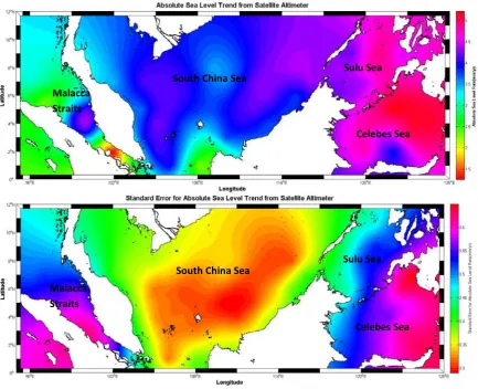
3.3 Analysis of the Absolute Sea Level Trend Mapping of the Malaysian Seas
As shown in Figure 11, the map of absolute sea level trend over the Malaysian seas as well as the map of standard errors for absolute sea level trend from satellite altimeter is produced respectively. As mapped in the Figure 9, offshore or deep ocean areas are the focal point when extracting points from altimeter because the residual of SLA increases closer to the coast due to the increased sea level variability in shallow depth water (Andersen and Scharroo, 2011).
The outcomes clearly show that the absolute sea level trend is rising and varying from place to place over the Malaysian Seas. The rate of sea level varies and gradually increases from east to west of Peninsular Malaysia. Meanwhile, for Sabah and Sarawak, the Sulu and Celebes Seas has a mixed tide prevailing semidiurnal characteristics and have a higher absolute sea level rise than other locations. This may due to the Sulu Sea is an
enclosed sea as it is isolated from the surrounding waters by a chain of islands (Din, 2014):
Table 4. Summary of the absolute sea level rate over the Malaysian Seas
Group Sea Level Rate (mm yr-1)
Malacca Straits 3.14 ± 0.12 South China Sea 3.85 ± 0.05
Sulu Sea 4.56 ± 0.14
Celebes Sea 4.81 ± 0.15
Total Average 4.09 ± 0.12
Based on Table 3, the Malacca Straits has the lowest absolute sea level rate, which is at 3.14 ± 0.12 mm yr-1. The depth and shape of Malacca Straits consist of a shallow rather narrow, the short term circulation dynamics seem to not average out over this area, because the mean sea level is somewhat disturbing annual cycle with lots of higher harmonics (Din et. al., 2012). SC38, South China Sea, Rate: 3.99 ± 0.35 mm yr-1
b)
SU07, Sulu Sea, Rate: 4.20 ± 0.45 mm yr-1
CE08, Celebes Sea, Rate: 4.86 ± 0.54 mm yr-1 c)
Figure 11. Map of absolute sea level trend (upper) and its standard error (lower) over the Malaysian Seas
The sea level rise at 3.85 ± 0.05 mm yr-1 in the South China Sea, which has a typical marginal sea characterized with a deep basin, shelf break, and shallow shelf. Meanwhile the Sulu Sea and Celebes Sea shows indicates a rather higher sea level rate compared to Malacca Straits and South China Sea, which is at 4.56 ± 0.14 mm yr-1 and 4.81 ± 0.15 mm yr-1 subsequently.
The acceleration of sea level rise for the Malaysian seas from the year 1993 to 2015 concludes that it has been accelerated at a rate of 4.09 ± 0.12 mm yr-1.
4. CONCLUSION
By having enough confidence in the data and selecting the best methods for processing all the data together from the year 1993 until 2015, Malaysian seas has been accelerating at the rate 3.14 ± 0.12 mm yr-1 to 4.81 ± 0.15 mm yr-1 for the chosen sub-areas, with an overall mean of 4.09 ± 0.12 mm yr-1 (solely based on the altimetry data). This overall mean of sea level rate for the Malaysian seas seem to slightly drop than the sea level rate from Din (2014) which is from the year 1993 to 2011, the rate of sea level rise is 4.56 ± 0.65 mm yr-1.
The sea level rate also is higher than the published values by AVISO’s Sea Level Research Team (2016), where from the year 1993 to 2015, the global sea level rise is estimated at a rate of 3.39 mm yr-1 using a combination of Topex/Poseidon, Jason-1 and Jason-2 altimetry data. It can be clarified that strong
El-Niño event that occur in the year 2015 somewhat affects the rate of sea level over Malaysian seas to drop abruptly.
Therefore, the information about sea level trends in this region is indeed valuable for the coastal management, town development, and flood mitigation. It is also important to be used for projecting the sea level rise for their relevance for future regional climate. A coastal area with the sea level rise projection information can be used to prevent from coastal erosion, and coastal inundation.
ACKNOWLEDGEMENTS
The authors are grateful to TU Delft, Permanent Service for Mean Sea Level (PSMSL) and Department of Survey and Mapping Malaysia (DSMM) for providing altimetry and tidal data respectively. This research is funded by the Ministry of Higher Education (MOHE) under the FRGS Fund, Vote Number R.J130000.7827.4F706.
REFERENCES
Akdag, C. (1996). Tidal Analysis of the South China Sea. Technical Report; Delft Hydraulics. Group of Fluid Mechanics, Faculty of Civil Engineering, Delft University of Technology.
Andersen, O. B. and Scharroo, R. (2011). Range and Geophysical Corrections in Coastal Regions: And Implications
Malacca
Straits
Malacca
Straits
South China Sea South China Sea
Sulu Sea
for Mean Sea Surface Determination. In Coastal Altimetry. Springer. DOI:10.1007/978-3-642-12796-0.
AVISO (2016). AVISO Satellite Altimetry Data. http://www.aviso.altimetry.fr/en/data/products/ocean-indicators products/mean-sea-level.html (30 April 2016)
Azhari Mohamed (2003). An Investigation of the Vertical Control Network of Peninsular Malaysia using a Combination of Levelling, Gravity, GPS and Tidal Data. Doctor of Philosophy, Universiti Teknologi Malaysia, Skudai.
Church, J. A., White, N. J., Aarup, T., Wilson, S. T., Woodworth, P. L., Domingues, C. M., Hunter, J. R. and Lambeck, K. (2008). Understanding Global Sea Levels: Past, Present and Future. Integrated Research System for Sustainability Science and Springer. Sustain Sci., DOI 10.1007/s11625-008-0042-4.
Church, J. A. and N.J. White (2011), Sea-level rise from the late 19th to the early 21st Century. Surveys in Geophysics, 32(4-5), 585-602, DOI: 10.1007/s10712-011-9119-1.
Din A. H. M. (2010). Sea Level Rise Estimation using Satellite Altimetry Technique. MSc Thesis, Universiti Teknologi Malaysia, Skudai.
Din, A. H. M., Omar, K. M., Naeije, M. and Ses, S. (2012). Long-term Sea Level Change in the Malaysian Seas from Multi-mission Altimetry Data. International Journal of Physical Sciences Vol. 7(10), pp. 1694. DOI: 10.5897/IJPS11.1596.
Din A. H. M. (2014). Sea Level Rise Interpretation in Malaysia using multi-sensor techniques PhD Thesis, Universiti Teknologi Malaysia, Skudai.
Fu, L. L. and Cazenave, A. (2001). Altimetry and Earth Science, a Handbook of Techniques and Applications. Vol. 69 of International Geophysics Series.
Hay C. C., Morrow E., Kopp R. E., and Mitrovica, J. X. (2015). Probabilistic reanalysis of twentieth-century sea-level rise, Nature, pg 481-484, DOI: 10.1038/nature14093.
Holland, P. W. and Welsch, R. E. (1977). Robust Regression using Iteratively Reweighted Least-squares. Communications in Statistics—Theory and Methods 6 (9), 813–827.
Intergovernmental Panel on Climate Change (IPCC). (2014). Synthesis Report. Contribution of Working Groups I, II and III to the Fifth Assessment Report of the Intergovernmental Panel on Climate Change [Core Writing Team, R.K. Pachauri and L.A. Meyer (eds.)]. IPCC, Geneva, Switzerland, 151 pp
PSMSL (2016). Permanent Service for Mean Sea Level. http://www.psmsl.org/ (29 January 2016)