SCAN PROFILES BASED METHOD FOR SEGMENTATION AND EXTRACTION OF
PLANAR OBJECTS IN MOBILE LASER SCANNING POINT CLOUDS
Hoang Long Nguyen a*, David Belton a, Petra Helmholz a a
Department of Spatial Sciences, Curtin University, Perth, WA, Australia -
[email protected]; [email protected]; [email protected]
Commission III, WG III/2
KEY WORDS: mobile laser scanning, point clouds, segmentation, planarity, scan profiles
ABSTRACT:
The demand for accurate spatial data has been increasing rapidly in recent years. Mobile laser scanning (MLS) systems have become a mainstream technology for measuring 3D spatial data. In a MLS point cloud, the point clouds densities of captured point clouds of interest features can vary: they can be sparse and heterogeneous or they can be dense. This is caused by several factors such as the speed of the carrier vehicle and the specifications of the laser scanner(s). The MLS point cloud data needs to be processed to get meaningful information e.g. segmentation can be used to find meaningful features (planes, corners etc.) that can be used as the inputs for many processing steps (e.g. registration, modelling) that are more difficult when just using the point cloud. Planar features are dominating in manmade environments and they are widely used in point clouds registration and calibration processes. There are several approaches for segmentation and extraction of planar objects available, however the proposed methods do not focus on properly segment MLS point clouds automatically considering the different point densities. This research presents the extension of the segmentation method based on planarity of the features. This proposed method was verified using both simulated and real MLS point cloud datasets. The results show that planar objects in MLS point clouds can be properly segmented and extracted by the proposed segmentation method.
1. INTRODUCTION
The demand for accurate spatial data has been increasing rapidly in recent years. Thanks to Global Navigation Satellite System, laser scanning, imaging and information technologies, mobile mapping technology has rapidly developed since the late 1980s. A mobile laser scanning (MLS) system allows us to observe 3D measurements of objects at a close range from a vehicle. Its allow users to collect precise point cloud data at normal road speed and capture scenes and details of objects more comprehensively than traditional satellite mapping or surveying. Therefore, MLSs have become a mainstream technology for measuring 3D spatial data.
Point cloud segmentation is the process of grouping spatially connected points that have similar characteristics. The outcomes are a number of separate segments or extracted features from the point clouds. Segmentation is a crucial step for many applications such as modelling features, registration or calibration. Because planar features are dominate in manmade environments, they are widely used in point clouds registration and calibration processes (Chan et al., 2013; Rabbani et al., 2007). Therefore, this paper focuses on the segmenting of planar features in MLS point clouds.
A number of different approaches have been proposed to segment planar features in laser point clouds. They can be divided into five groups: edge based (Huang & Menq, 2001), robust model fitting (Fischler & Bolles, 1981; Hough, 1962; Oesau et al., 2016; Vosselman & Maas, 2010), scan line based (Jiang & Bunke, 1994; Sithole & Vosselman, 2003) and region/surface growing based (Nurunnabi et al., 2012; Nurunnabi et al., 2015; Oesau et al., 2016; Rabbani, van den Heuvel, & Vosselmann, 2006; Vosselman & Maas, 2010).
* Corresponding author
In edge based approaches, the edges and boundary points have to be determined first. Then, points inside the boundaries are group into region. However, finding closed boundaries is not always feasible due to noise, sampling, complex surfaces.
In robust model fitting groups, RANSAC is possibly the most popular method in extracting planar objects in point clouds data due to the simplicity and robustness,. However, one the parameters required for RANSAC is highly dependent on the magnitude of noise which cannot always be predicted. Furthermore, depending on this threshold points near the boundary of two adjacent objects may be labelled to either of these two objects. Deschaud and Goulette (2010) drew the conclusion that while RANSAC provides a very good outcome for the detection of large planes in noisy point clouds, it is not efficient in detecting small planes in large point clouds.
Scan line base segmentation breaks each scan line into smaller scan profiles and then merge scan profiles of the same surface based on certain criteria. An approach for segmenting range images into planar patches was proposed by Jiang and Bunke (1994). Sithole and Vosselman (2003) proposed a method to segment Air-borne Laser Scanning (ALS) point clouds. This method uses 2D profiles sampled in different directions. These profiles are generated by connecting points that satisfy some conditions. However, connecting points by comparing their height or slope is not suitable to form line segments of vertical planar objects, which are dominate in MLS point clouds. .
the edge based approaches (Nurunnabi et al., 2015). Oesau et al. (2016) proposed a method for planar object detection for unorganized point clouds. Their method uses the K-nearest neighbour (KNN) for determining the neighbours for normal vectors estimation. As discussed in Nguyen et al. (2015) KNN is not suitable for this task when applying to MLS sparse point clouds. Rabbani et al. (2006) proposed a segmentation method for terrestrial laser scanning point clouds using smoothness constraints. This method groups connected points based on their direction vectors. Principal Component Analysis (PCA) is used to estimate the normal vectors of points from their neighbours. Neighbouring points are determining by using k-nearest neighbour (KNN) or fixed distance neighbour (FDN) algorithm. Seed points for region growing are selected based on their residuals. As PCA is very sensitive to outliers, Nurunnabi et al. (2015) proposed the Robust and Diagnostic PCA (RDPCA) method to detect outliers and then estimate local saliency features from the clean subset. A robust segmentation method based on the estimated local saliency features was proposed to segment dense and homogeneous mobile laser scanning point clouds. However, the robust segmentation method based on RDPCA fails in segmenting sparse and heterogeneous MLS point clouds (Nguyen et al., 2015).
Nguyen et al. (2015) proposed two approaches for segmentation of sparse and heterogeneous MMS point clouds: (1) segmentation method based on scan profile and RDPCA, and (2) Region Growing based on the Planarity of Scan profiles (RGPL). Although, the outcomes of these two methods give promising results, they can only be applied for MLS point clouds under certain conditions which are not met for all MLS point cloud datasets. Furthermore, these two approaches were only verified by using the point clouds of a pre-designed target.
The robust segmentation method based on RDPCA proposed by Nurunnabi et al. (2015) could be used for dense MLS point clouds, and the two approaches proposed by Nguyen et al. (2015) could be used for the spare and heterogeneous MLS point clouds. However, there are no guidelines concerning the range of point cloud densities that each of the approaches can handle so as to determine which is best to apply.
This research proposes a new segmentation method that can be applied to all types of captured point clouds from MLS systems with 2D laser scanners. This research extends the work of Nguyen et al. (2015) by improving the neighbourhood selection method for direction vectors estimation (e.g. by considering the scan line indices), improving the scan profiles growing process to deal with some problems (e.g. two different scan profiles that have similar direction vectors) that were not take into account in the original version. Then, a method is proposed for solving the case of changing vehicle speeds. Finally, the extension will be validated using both simulated and new real datasets. The RGPL method was compared with the segmentation method based on RDPCA in Nguyen et al. (2015). Instead, this paper focuses only on the extent RGPL method and its applicability for all type of MLS point clouds without to compare the performance of this method with other segmentation methods.
This paper is organized as follows, section 2 presents the background of this research, and section 3 presents the extension of the RGPL. Next, a description of the datasets that are used to verify the propose method and the results are presented in section 4, along with discussions. The paper closes with the conclusion and possible future work.
2. BACKGROUND
2.1 Point density of a MLS point cloud
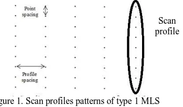
Traditionally, point density of a point cloud is defined as the number of points per some area unit. The captured 3D point clouds of a MLS system (MLSs) that uses 2D laser scanner(s) as the imaging sensor(s) are derived by utilising the movement of the carrier vehicle. A scan line is a full circle of scan. A scan profile or segment contains a group of points of the same scan line on the same surface. Scan profiles of the same planar surface are normally parallel with each other. According to Cahalane et al. (2014) and (Nguyen et al., 2015) different surfaces in the same point cloud may have different point densities. Point densities of a surface in the same point clouds can be defined as the distance between two adjacent scan profiles or profile spacing and the distance between two adjacent points of the same scan profile or point spacing (Figure 1).
Currently, a number of MLSs are available on the market. Several MLSs have been reviewed in Puente et al. (2012). They have different configurations as well as scanning patterns. With regard to scanning patterns, MLSs can be categorised into two classes: MLSs that have laser head(s) placed perpendicular (type 1) and MLSs that have laser scanner(s) placed oblique (type 2) to the trajectory of the carrier vehicle. Point clouds captured by two different MLS classes have different scan line patterns. This research focuses on scanners of type 1. Furthermore, point clouds of the same feature collected at the same speed by different MLSs will have different densities due to the different configurations of different MLSs. For instance the MDL Dynascan S250 (Renishaw, 2015) has a single laser head with a low scanner rate (e.g. 20 Hz) and a low scanner pulse rate (e.g. 36000 pts /sec). Meanwhile, the RIEGL VQ-450 (RIEGL, 2015) is equipped with a laser head with a high scanner rate (e.g. 200 Hz) and a high scanner pulse rate (e.g. up to 550000 points / sec). The specifications of MDL Dynascan S250 and RIEGL VQ-450 are shown in Table 1. Consequently, at the same speed the profile spacing of the point cloud of the same object collected by RIEGL VQ-450 can be ten times narrower than the profile spacing of the point cloud captured by MDL Dynascan S250. The point spacing of the same object at the same distance captured by RIEGL VQ-450 can be fifteen times smaller than the one collected by MDL Dynascan S250.
Figure 1. Scan profiles patterns of type 1 MLS
MDL Dyanscan S250
RIEGL VQ-450
Range up to 250 m up to 800 m
Scanner rate up to 20 Hz up to 200 Hz Scanner pulse rate 36,000 pps 550,000 pps
Accuracy 1 cm 8 mm
Table 1. MDL Dynascan S250 and RIEGL VQ-450 specifications
To conclude, depending on the speed of the vehicle when scanning, the specifications of the MLS and the several factors mentioned above, captured point clouds of the interest features can be sparse or dense. The point spacing can be smaller or can be bigger than the profile spacing.
3. METHODOLOGY
In this section the extension of the RGPL segmentation method applicable to all type of captured point clouds from MLS system with 2D laser scanners is introduced. Unlike other region growing methods, the RGPL utilizes the direction vectors of points instead of normal vectors of points, then using planarity value to group points of the same surface. The direction vector of a point is defined as the vector that is parallel with the direction of the scan profile this point belongs to. It can be estimated via the eigenvector corresponding to the biggest eigenvalue of the covariance matrix formed by a point and its neighbours of the same scan profile. The details of the RGPL is described in (Nguyen et al., 2015). In this paper, the RGPL is improved by proposing a new neighbouring selection method for direction vectors estimation, developing method for solving the case of changing speeds, and solving the issue with complex structures.
3.1 Breaking scan lines into scan profiles
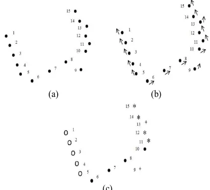
According to Nguyen et al. (2015) point clouds can be broken into scan profiles based on the direction vectors of points. As different objects in the same point cloud may have different point densities, the K-nearest neighbour algorithm is not suitable for selecting neighbouring points for direction vectors estimation. In order to estimate direction vectors of points, neighbours need to be selected from the same scan profile. If the points spacing of all interest features are much smaller than their profiles spacing and the profile spacing is stable during the scan, in the original RGPL (Nguyen et al., 2015) Fixed distance neighbour (FDN) is proposed to obtain neighbouring points for estimating direction vectors. However, this FDN cannot be applied when the velocity of the carrier vehicle is changed during the scans or the scan line spacing is not much bigger than the points spacing. In order to solve this problem, this paper proposes a new approach for breaking point clouds into different scan profiles by first splitting them into scan lines (section 3.1.1). Then, neighbouring points of each point are determined. After that a modified RANSAC line fitting method is applied in order to determine the ‘clean’ subset (section 3.1.2). Based on this subset, the direction vector of each point is calculated by using PCA (Figure 2 (b)). Finally a scan profiles growing process (section 3.1.4) is performed leading to the segmented scan lines and remove outliers (e.g. 9th and 13th points) (Figure 2 (c)).
3.1.1 Splitting point clouds into scan lines: Normally, with some MLS systems, the final output includes the information about the scan line and captures time of each point. In this case, points on different scan lines can be easily split into different groups. However, with some systems (e.g. MDL Dynascan S250) this information is not readily provided. Fortunately, points in a collected point cloud are often stored in sequence of capture. Hence, if the scanner positions of each scan are also stored in the captured point clouds, each scan line can be split based on these scanner positions (Figure 2 (a)). The scanner positions are the X, Y, Z coordinates of the centre of the laser scanner at the scanning epoch.
(a) (b)
(c)
Figure 2. Breaking a scan line into different scan profiles: (a) points on a scan line; (b) direction vectors of each point and (c) the final outcome (different symbols indicate different scan profiles)
3.1.2 Direction vector estimation: There are two steps required in order to estimate direction vector of a point. They are described as follows:
Step 1 - Local neighbourhood selection: FDN is not suitable in directly applying to the MLS point clouds collected at different speeds to determine neighbour for direction vector estimation as the direction vector of a point needs to be estimated from neighbours on the same scan profile with this point. However when the point clouds are split into scan lines, the KNN or FDN algorithm can be applied on each scan line to determine the neighbours of each point that belong to the same scan line. Selecting neighbours only from the same scan profile with the selected point is impossible when this point is near an intersection of two different scan profiles. If KNN or FDN is used the number of neighbours lie on the same scan profile with the selected point may be less than those on other scan profile depending on the profile spacing’s of the two different scan profiles. This may cause a problem when estimating the direction vector of this point. Therefore, a more suitable selection method needs to be applied. Because captured points of a scan line are normally stored in sequence it can be assured that at least half of the neighbours will be selected from the same scan profiles with the selected point by utilizing the indices of the captured points. As a result the number of inliers is always bigger than the number of outliers. Furthermore, changing the number of neighbours will not impact on the results of direction vectors estimation process significantly. For instance, neighbours can be selected from five neighbouring points captured before and after the selected point.
iteration T. The Tr can be set based on the accuracy of the
scanner. The number of required iterations to ensure a good solution is not as significant as the original RANSAC. This is because the random selections of points are constrained. For points not near the intersection of two different scan profiles, any two sample points, except noise points, can be used to determine the consensus set for direction vector estimation. However, for points near the intersection, it can belong to either one of the two scan profiles. Therefore, the query point and the closest points captured before are used for the first iteration. The query point and the points captured after are used as random samples for the second iteration. However, to prevent the case where these two closest points are influenced by noise, more iteration steps are needed to produce a good direction value. Random samples for each of these additional iterations are selected from either neighbouring points captured after or before.
3.1.3 Scan profiles growing: After the direction vectors of all points are calculated (section 3.1.3), a scan profile growing process is performed to group points of the same profile based on their direction vectors. This process is as follows: P denotes all the points in the point cloud, and the point Pi that has the smallest point index is selected as the seed point for the new scan profile. It is added to the seed point group Sc and the current scan profile SPc, and removed from P. If two neighbour points belong to the same scan profile, they must not only have the same direction vector, but also belong to the line going though one point and parallel to the direction vector. In fact, in most of the case using the first two thresholds is enough to determine the scan profiles.
However, in order to prevent the case when two surfaces that have the same plane equation and adjacent to each other in horizontal direction, a maximum distance between two neighbour points of the same scan profile is also needed to be set. Theoretically, as the distances between any two adjacent points on the same scan profile is identical, this threshold should be set equal twice the distance between two first seed point of the scan profile (i.e. the point spacing of this scan profile). However, this parameter should be set to be equal four times the point spacing due to possibility of the presence of noise and the imperfect measurements from the scanner. Therefore, the angle between the direction vector of Pi and Pi+1, the distance DLi from Pi+1 to the straight line that goes though Pi and parallel to the direction vector of Pi, and the distance Di between Pi and Pi+1 are calculated.
Next, if all of the three calculated values are smaller or equal than thresholds, Pi+1 is added to the seed point group Sc and the current scan profile SPc, and removed from P. if one of the calculated value is bigger than predetermined thresholds, it means Pi+1 and Pi do not belong to the same scan profile. Then, SPc will be saved, and SPc and Sc will be cleared. After a complete scan profile is formed, the seed point for the next scan profile is selected from the remaining points in Pthat has the smallest point index. The process is repeated until all points are assigned to different scan profiles. As shown in Figure 2 (c), noise (e.g. 9th and 13th points Figure 2 (c)) can be removed
by the direction vectors of points. This process can be summarized in Algorithm 1 as follows.
Algorithm 1:
Input: X, Y, Z coordinates of points in point clouds P and their direction vectors DP
Output: a scan profile list SP
3.2 Grouping Scan profiles
In MLS point clouds, if different profiles belong to the same planar surface, they are parallel. However, if two scan profiles are parallel, it does not mean they belong to the same planar surface. They can belong to different planar surface that have similar orientation with the ground surface. Therefore, the outcomes of this step are considered as grouping the scan profiles that potentially belong to the same surface. This can be done by checking the angle between direction vectors of different scan profiles with each other. In theory, due to imperfect measurements of the scanner, two scan profiles of the same surface will also not be perfectly parallel. Furthermore, as the carrier vehicle trajectory is not always straight, therefore, a threshold is needed to be set. If the calculated angle between the direction vectors of two scan profiles is smaller than a threshold, they are considered as parallel with each other.
3.3 Segmentation method based on planarity RGPL
RGPL chooses seed scan profiles based on the number of neighbours. Hence, in case a point cloud is collected at different speeds, a fixed radius parameter cannot be applied for the whole group of scan profiles determined from section 3.2. These groups must be once again split into smaller different groups. If the information about the speeds and the time stamps for the collected point are known, these groups can be split based on this information. However, with some systems, such as the MDL Dynascan S250, this information is not provided. Consequently, users have to manually split the point cloud into smaller sub-point clouds that are collected at similar speeds. In order to alleviate this problem, this paper proposes a method to split these groups of scan profiles based on the distances between the scan profiles.
First, all the distances of the scan profile to its closest scan profiles are calculated. They can be derived by a simple KNN algorithm. In a sparse point cloud, a thin pole can be represented by a single scan profile, hence a threshold can be set to prevent surface with only one Scan profile being produced. As a result, they can be removed from the group. As the aim is to group scan profiles scanned from high to low speed, and the faster the speed, the longer the profile spacing, this approach starts by determining the seed scan profile which has the longest distance to its closest neighbour. Then, the number of neighbours of each scan profile, with the radius smaller than the longest distance can be calculated by a simple FDN algorithm. Scan profiles that have less than three neighbours are put into a new group and removed from the original group. The reason for this is that if scan profiles have more than two neighbours, they definitely are collected at a much lower speed. All of the scan profiles in the new group are considered to be collected at similar speeds. As discussed in section 2, the scan profile spacing of different surfaces captured at the same speed can be different. Therefore, the outcomes of this process is not only to split the scan lines collected at different speeds but also to separate the scan profiles of different surfaces that do not have similar orientations into different groups.
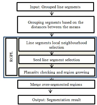
3.3.2 RGPL: RGPL aims to segment point clouds by checking the planarity between different scan profiles instead of checking normal vectors of each point like other region growing methods (Nurunnabi et al., 2012; Rabbani et al., 2007). In addition, the assumption is made that each planar feature in the point clouds has at least two scan profiles. This assumption is needed because at least two scan profiles of features are required to detect planar features. Based on this, each group of Scan profiles is segmented based on pre-defined rules. This method’s workflow is shown in Figure 3.
After grouping scan profiles that were collected at similar speeds, the RGPL process can be applied to segment point clouds. The RGPL process is summarized as follows. RGPL starts by determining a seed scan profile which has one neighbouring scan profile. The number of neighbours of each scan profile in each group can be considered as the neighbourhood size of the mean point of the selected Scan profile, with mean points of other Scan profiles within a pre-defined range. It can be calculated by a simple FDN algorithm with the radius close to twice the scan line spacing. If the selected scan profile has only one neighbouring scan profile within a distance less than twice the scan line spacing, and as a planar surface has to have at least two scan profiles, then these two parallel scan profiles will be assigned to the same planar surface. If it has two neighbours, the planarity of points on these three scan profiles will be checked by using PCA. The planarity of a group of points is considered as the smallest eigenvalue of the covariance matrix formed by those points. A perfectly smooth planar surface will have its planarity value equal to zero. However, in reality, most planar surfaces are not perfectly smooth. Furthermore, the planarity value is also influenced by the accuracy of the scanner. Therefore, a threshold for checking the planarity needs to be set. If the calculated planarity is smaller than a pre-defined threshold, they will belong to the same plane.
For good segmentation results, scan profiles near the boundaries of different surfaces need to be analysed carefully. In a real point cloud, it may be the case that one of the collected scan profiles lies very close to the boundary of two adjacent planar surfaces that have similar orientations to the ground surface. Scan profiles of these two adjacent planar surfaces are assigned in the same group (3.2). The planarity calculated from points on this scan profile and other point from the two adjacent surfaces
may both be smaller than the predefined threshold. Consequently, this scan profile can belong to both of the two surfaces. Changing the value of the threshold to be bigger than one value and smaller than the other could be a solution for this problem. However, determining a threshold that works for every case in the same collected point clouds is almost impossible. In addition to this, setting the planarity threshold too small may lead to over-segmentation cases. Hence this planarity threshold needs to be carefully set. Depending on the users’ requirements, this threshold should be set to be big enough to recognize the required most rough surfaces. Then, if a segmented surface – surface A have an adjacent surface – surface B, the planarity of the surface formed by surface B and the last scan profile of surface A will be calculated. Finally, this value will be compared with the planarity of surface A. If this value is smaller than the planarity of surface A, the last scan profile of surface A will assigned to belong to surface B.
3.3.3 Problem when using mean points to determining neighbouring scan profile: Using distances between mean points of scan profiles instead of ‘true distance’ between scan profiles can reduce the processing time. However, this approach also has drawbacks. For example, if there are some objects (e.g. cars, phone boxes) in front of building facades. Points on these objects occlude the facades meaning points are missing from the scan lines for these facades. Consequently, mean points of those scan profiles will change. If a wall has windows or some objects on it, the scan profiles of the wall for this area will be broken into several scan profiles. This will also lead to changes in distances between mean points of different scan profiles. Therefore, neighbouring scan profiles of the same object may be not considered as neighbours of each other. Consequently, they are labelled as different regions.
indexes of the beginning and ending scan line of each region need to be determined. Two regions are considered as neighbours of each other if the ending scan line of one region is adjacent to the beginning scan line of the other. Finally, the planarity of these two regions is calculated. If this value is smaller than a threshold, they will be merged. Then, the beginning and ending scan line indexes of this new region are recalculated. This process is iteratively performed until all the regions are checked. The planarity threshold can be set equal to the planarity threshold of the RGLP. By performing this process, a threshold (e.g. 10 degrees) for grouping different scan profiles as discuss in section 3.2 can be fixed for all point clouds.
4. RESULTS AND DISCUSSION
4.1 Datasets
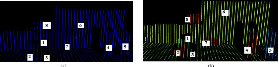
Two datasets are used in order to verify the proposed segmentation method. The first dataset is an errorless simulated point cloud of a house facade with a window and a door. The dataset has heterogeneous point density with the profile spacing’s vary from 0.008 to 0.095 metre and point spacing’s vary from 0.01 to 0.014 (Figure 5 (a)). The second dataset is the point cloud captured near a supermarket near the Curtin University Bentley campus in Australia using the MDL Dynascan S250. There are 8 planar surfaces in this area (Figure 6(a)), including three surfaces of the target that are used for registration (1, 2 and 3), two phone boxes (4 and 5), 1 façade of the supermarket building (6), 1 small planar object (7) that has different surface normal vector and adjacent to supermarket façade, and 1 façade of an air condition (8) near the supermarket. Surface 8 has similar surface normal vector with surface 6. Nguyen et al. (2015) claimed that the robust segmentation based on RDPCA (see section 1) fails in segmenting the sparse point clouds of this target (surfaces 1, 2 and 3).
4.2 Evaluation of the proposed segmentation method
4.2.1 Evaluation of splitting point clouds into scan lines: In this research, the captured point clouds were split into different scan lines based on the laser positions. By using laser position points as “break points”, captured point clouds can be segmented into different scan lines.
4.2.2 Evaluation of breaking scan lines into different scan profiles: Theoretically, the angle threshold should be set to be small (e.g. 5 degrees). In order to investigate the influence of the three (e.g. the neighbourhood size, the angle threshold and the number of iteration) of five required parameters to the outcomes of this process, different value of these parameters were applied. For instance, the neighbourhood size parameter is set to 10 (i.e. 5 points captured before and 5 points captured after), 12 and 14; the angle threshold were set 5, 7 and 10 degrees as in reality, the angle between two vertically adjacent surfaces is normally smaller than 10 degrees; the threshold Di for maximum distance between two points of the same scan profile is set to three, four, five times the point spacing; and the number of iterations T was set to 5, 7 and 10 for both datasets. The threshold for the modified RANSAC line fitting, Tr and DLi
was set to 0.02 metre, twice the range accuracy of the MDL Dynascan S250 mobile laser scanning (0.01 metre) (Table 1); As dataset 1 is free of noise and error, with different parameters values, the outcomes of this process are identical. While with dataset 2, they are not identical but very similar to each other. Figures 5 (b) shows examples of the outcomes of dataset 1 after breaking into different scan profiles.
4.2.3 Evaluation of grouping line segments: As discussed in section 3.3.4, the angle threshold for grouping scan profiles was set 10.0 degrees for both dataset2 1 and 2. However, three different values (7, 10 and 15 degree) were applied to validate the discussion in 3.3.4. In fact, parallelism is just one of the required conditions to group different scan profiles into the same surface. Furthermore, two scan profiles close together are normally parallel (i.e. they belong to the same surface)/ Therefore, changing the values of this parameter will cause almost no change to the final result of RGPL. Figure 5 (c) shows the outcome of grouping process of the dataset 1 with the angle threshold was set to 10 degrees. Scan profiles that have similar direction vectors are put into the same group.
4.2.4 Evaluation of the RGPL method: For the RGPL method, the threshold for checking the planarity is depended on the roughness of the surface of the planar feature and the accuracy of the scanning system. As dataset 1 is errorless the planarity threshold can be set equal to zero. Empirically, the planarity parameter was set to 0.0002 for dataset 2. The planarity threshold for dataset 2 was also applied for dataset 1 to investigate its influence. In dataset 1, as the points density of this dataset is heterogeneous – different profile spacing. The points on the same features are assigned into different regions. In dataset 2, most of the features were successfully segmented except the façade of the supermarket building. Due to the present of the two phone boxes and the target in front of the façade of the supermarket building, points on this surface were assigned into different regions. These over-segmented problems occur due to the reasons discussed in section 3.3.3 and 3.3.4.
Parameters Values Comments
Neighbourhood size 10, 12, 14 Can be fixed for all point clouds
0.02 metre Depending on the accuracy of the scanner
Line Fitting 0.02 metre Depending on the accuracy of the scanner
Planarity value 0.0002 Defined by experiment
Table 2. Used Parameters for RGPL
surfaces. A conclusion can be drawn from these results that a planarity threshold can be applied for a whole point cloud. All used parameters of RGPL are summarized in Table 2. All but one can be easily automatically determined. However, the planarity value needs to be empirically determined to recognize the roughest surface in the scan area.
5. CONCLUSION AND OUTLOOK
The point density of captured point clouds depends on several factors that are important when extracting features. It can be sparse or can be dense. The point spacing can be smaller or can be bigger than the profile spacing. This paper proposes an extension of the RGPL segmentation method. The proposed method was verified with both a simulated dataset and a real dataset captured by MDL Dynascan S250. The segmentation results show that this proposed segmentation method is successful in segmenting MLS point clouds. Although, only point clouds for a type 1 scanner are used to verify, the
proposed approach is suitable for segmenting point clouds captured by type 2 scanners once the different geometry is accounted for. Nine parameters are required in this segmentation method, five of them (e.g. the angle threshold for scan profile growing, the number of neighbours, the number of iteration, the maximum distance for scan profiles growing and the angle threshold for grouping) do not give significant impact to the results. Therefore standard values for these five parameters as described in Table can be used for all point clouds. Meanwhile RANSAC threshold and line fitting threshold can be defined based on the accuracy of the scanner.
Future work will investigate the possibility of dynamic definition for the planarity threshold and extend the proposed methods to segment others features (e.g. cylinders, spheres). Finally, this proposed method should be validated on other datasets from MLSs that have oblique scanner(s) (e.g. the MDL Dynascan S250X).
(a) (b) (c) (d)
Figure 4. RGPL result for dataset 1: (a) point cloud; (b) different scan profiles; (c) group of parallel scan profiles; (d) final result. Different regions are indicated by different colours
(a) (b)
Figure 5. RGPL result for dataset 2: (a) point cloud; (b) final result. Different regions are indicated by different colours
REFERENCES
Cahalane, C., McElhinney, C. P., Lewis, P., & McCarthy, T. (2014). Calculation of Target-Specific Point Distribution for 2D Mobile Laser Scanners. Sensors (Basel, Switzerland), 14(6), 9471-9488.
Chan, T. O., Lichti, D. D., & Glennie, C. L. (2013). Multi-feature based boresight self-calibration of a terrestrial mobile mapping system. ISPRS Journal of Photogrammetry and Remote Sensing, 82(0), 112-124.
Deschaud, J.-E., & Goulette, F. (2010). A fast and accurate plane detection algorithm for large noisy point clouds using filtered normals and voxel growing. Paper presented at the Proceedings of the 5th International Symposium 3D Data Processing, Visualization and Transmission, Paris, France.
Fischler, M. A., & Bolles, R. C. (1981). Random sample consensus: a paradigm for model fitting with applications to
image analysis and automated cartography. Commun. ACM, 24(6), 381-395.
Golovinskiy, A., Kim, V. G., & Funkhouser, T. (2009). Shape-based Recognition of 3D Point Clouds in Urban Environments. Paper presented at the International Conference on Computer Vision ICCV.
Hough, P. V. C. (1962). Method and means for recognizing complex patterns: Google Patents.
Huang, J., & Menq, C.-H. (2001). Automatic data segmentation for geometric feature extraction from unorganized 3-D coordinate points. IEEE Transactions on Robotics and Automation, 17(3), 268-279.
Nguyen, H. L., Helmholz, P., Belton, D., & West, G. (2015). New methods for segmentation of sparse mobile laser scanning point clouds. Presented at the The 9th International Symposium on Mobile Mapping Technology (MMT 2015), Sydney, Australia.
Nurunnabi, A., Belton, D., & West, G. (2012, 3-5 Dec. 2012). Robust Segmentation in Laser Scanning 3D Point Cloud Data. Paper presented at the Digital Image Computing Techniques and Applications (DICTA), 2012 International Conference on.
Nurunnabi, A., West, G., & Belton, D. (2015). Outlier detection and robust normal-curvature estimation in mobile laser scanning 3D point cloud data. Pattern Recognition, 48(4), 1404-1419.
Oesau, S., Lafarge, F., & Alliez, P. (2016). Planar Shape Detection and Regularization in Tandem. Computer Graphics Forum, 35(1), 203-215. Puente, I., González-Jorge, H., Arias, P., & Armesto, J. (2012). LAND-BASED MOBILE LASER SCANNING SYSTEMS: A REVIEW. Int. Arch. Photogramm. Remote Sens. Spatial Inf. Sci., XXXVIII-5/W12, 163-168.
Rabbani, T., Dijkman, S., van den Heuvel, F., & Vosselman, G. (2007). An integrated approach for modelling and global
registration of point clouds. ISPRS Journal of Photogrammetry and Remote Sensing, 61(6), 355-370.
Rabbani, T., van den Heuvel, F. A., & Vosselmann, G. (2006). Segmentation of point clouds using smoothness constraint. Paper presented at the IEVM06.
Renishaw. (2015). MDL Dynascan S250. Retrieved 21/07, 2015, from http://www.renishaw.com/en/dynascan-s250--27332
RIEGL. (2015). RIEGL VQ-450. Retrieved 19/11, 2015, from http://www.riegl.com/uploads/tx_pxpriegldownloads/10_DataS heet_VQ-450_rund_2014-09-02.pdf
Sithole, G., & Vosselman, G. (2003, 22-23 May 2003). Automatic structure detection in a point-cloud of an urban landscape. Paper presented at the Remote Sensing and Data Fusion over Urban Areas, 2003. 2nd GRSS/ISPRS Joint Workshop on.