Use of spatially distributed water table
observations to constrain uncertainty in a
rainfall–runoff model
R. Lamb
a, K. Beven
b& S. Myrabø
c aInstitute of Hydrology, Wallingford, Oxfordshire, OX10 8BB, UK b
Environmental Sciences, Lancaster University, Lancaster, LA1 4YQ, UK c
Centre for Soil and Environmental Research, Jordforsk, N-1432 Aas, Norway
(Received 5 February 1998; accepted 23 June 1998)
The Generalised Likelihood Uncertainty Estimation (GLUE) methodology is used to investigate how distributed water table observations modify simulation and parameter uncertainty for the hydrological model TOPMODEL, applied to the Sæternbekken Minifelt catchment in Norway. Errors in simulating observed flows, continuously-logged borehole water levels and more extensive, spatially distributed water table depths are combined using Bayes’ equation within a ‘likelihood measure’ L. It is shown how the distributions of L for the TOPMODEL parameters change as the different types of observed data are considered. These distributions are also used to construct corresponding simulation uncertainty bounds for flows, borehole water levels, and water table depths within the spatially-extensive piezometer network. Qualitatively wide uncertainty bounds for water table simulations are thought to be consistent with the simplified nature of the distributed model.q1998 Elsevier Science
Limited. All rights reserved
Keywords: distributed hydrological models, TOPMODEL, uncertainty, water table predictions.
1 INTRODUCTION
Numerical experiments suggest limitations to the conven-tional approach to hydrological model calibration that seeks a unique optimum set of parameter values.5,10,14,27 It has been recognised in various contexts that, for a given set of observations, many parameter sets may often be found to produce similarly acceptable simulations, as defined in terms of some objective function. Typical examples are the appearance of a plateau, rather than a well-defined peak, in the response surface of the optimisation function or the presence of several, distinct optimal parameter sets in different regions of the parameter space. The general term ‘equifinality’ has been used by Beven5 to describe these problems. A further difficulty may arise if a model can be calibrated using several sets of observations (e.g. observations from different periods of time or of different variables). Experience suggests that regions of the parameter space corresponding to good
simulations are likely to change as different data sets are considered.
The appearance of equifinality can be interpreted as a source of simulation uncertainty arising directly from the interaction of parameters in a model and indirectly from errors in model structure and data. Multiple acceptable parameter sets were found21 during an application of the distributed model TOPMODEL to the Sæternbekken Minifelt catchment in Norway, where detailed water table observations have been made.23 In this paper, it is shown how these water table data have been used with rainfall and streamflow measurements to constrain the uncertainty of TOPMODEL simulations of the catchment.
The methodology used is the Generalised Likelihood Uncertainty Estimation (GLUE) procedure.4,7 GLUE is a Monte Carlo based technique that allows information from different sets of observations to be combined using Baye-sian principles to estimate simulation uncertainty. This is achieved through the computation of a likelihood measure
Printed in Great Britain. All rights reserved 0309-1708/98/$ - see front matter
PII: S 0 3 0 9 - 1 7 0 8 ( 9 8 ) 0 0 0 2 0 - 7
for many model realisations. It should be noted that the term ‘likelihood’ is used here in a broader sense than in classical likelihood statistics. Rather than estimating the likelihood or probability of certain observations given a model (assuming incidentally that a correct model is identifiable), we will interpret the likelihood measure for present purposes as an indication of the relative likelihood of a model being acceptable, given some observations.
The GLUE technique has been applied by Romanowicz
et al.25using a more conventional likelihood function devel-oped under the specific assumption of normally-distributed, first order autocorrelated errors, although this required a considerable computational effort.
This paper follows on from the work of Lamb,19 which was the first attempt to use spatially distributed field obser-vations of the water table within the GLUE framework. A similar approach has also been demonstrated by Franks
et al.,13using water level measurements from piezometers arranged in a transect in the Zwalm catchment, Belgium. Previous work by Binley and Beven7used synthetic water table data within GLUE, these data having been generated for a hypothetical hillslope using a detailed, 3D numerical flow model.
2 THE SAETERNBEKKEN MINIFELT CATCHMENT
The Minifelt is a small (0.75 ha) experimental catchment, situated approximately 250 m above sea level, on imperme-able bedrock, 10 km west of the city of Oslo. The catchment has been used to investigate runoff and shallow groundwater processes in the till based soils, for which a dense network of instruments was established.22
The data used in this paper are hourly observations of discharge (measured at a V-notch weir) and rainfall
(measured by a gauge located on the catchment boundary), hourly water levels from four logged boreholes, and water levels in 108 piezometers (measured manually). A detailed topographic survey was used to construct a digital terrain model (DTM) for the catchment at a 2 m 3 2 m grid
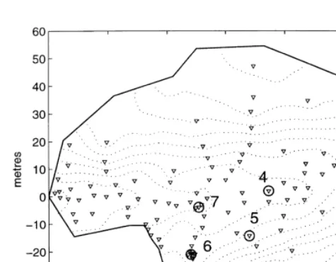
resolution. This DTM grid resolution was chosen in an attempt to obtain a detailed representation of hydrologically significant topographic features (at the hillslope scale) with-out introducing false topographic features as artefacts of the interpolation. The DTM was checked qualitatively in the field by visual inspection. The locations of instruments within the catchment are shown in Fig. 1 with contours derived from the DTM. Details of the field instrumentation are given by Myrabø.23
Runoff processes in the Minifelt are closely linked to the dynamics of the water table in the shallow (up to 1 m thick) soils. In particular, many parts of the catchment may become saturated under storm conditions. A variable source area concept of runoff production11,16,17is therefore appropriate. There is evidence from soil depth measure-ments that the extensive saturation may be caused in part by the reduction in lateral soil transmissivity where bedrock rises close to the surface, suggesting a return flow mechan-ism. Erichsen and Myrabø12 showed that topographic indices have some power to explain patterns of water table depths observed in the Minifelt. Although variation of soil properties must also influence the water table, topo-graphy has been adopted as the main control to allow the use of a simple model, outlined below.
3 DISTRIBUTED SIMULATION USING TOPMODEL
The variable source area mechanism for runoff production is represented in the distributed model TOPMODEL.1 The distribution of storage in the simplest form of TOPMODEL is determined by topography via the index ln(a=tanb), where a [dimension L] is the upslope drained area per unit contour width and tanb is the topographic slope, used to approximate the hydraulic gradient of the saturated zone. This index was calculated from the Minifelt DTM using an automated, multiple-flow direction algorithm.24
In the implementation of TOPMODEL used for this work, the local storage deficit due to gravity drainage, S [L], is given by
S¼S¯þm l¹ln a
tanb
(1) whereS [L] is the areal average of the local storage deficits,¯
l is the areal average of ln(a=tanb)and m [L] is a para-meter. The derivation6of eqn (1) depends on an assumption that fluxes in the saturated zone rapidly become uniform under uniform recharge and that the lateral transmissivity of the soil when just saturated has the same value, T0
[L2T¹1], throughout the catchment. The topographic index is expressed in logarithmic form because of a further
Fig. 1. Location of instruments in the Minifelt catchment.
Trian-gles indicate piezometer locations, numbered circles the position of the logged boreholes and ‘P’ the location of the rain gauge. The
assumption that transmissivity decreases exponentially with increasing storage deficit everywhere in the catch-ment. It can be shown6 that these assumptions are consistent with a description of the saturated zone as a lumped store, such that
QSZ¼Q0exp(¹S¯=m) (2)
where the specific discharge QSZ [L T
¹1] is the output
from the saturated zone, averaged over the catchment area, and
Q0¼exp(lnT0¹l) (3)
Because the soil transmissivity term T0 enters eqn (3) in
logarithmic form, the TOPMODEL transmissivity parameter will be taken to be the transformed variable, lnT0.
To obtain the local depth to the water table, z [L] from the storage deficit, S, a simple linear scaling is assumed where
z¼S=dv (4)
anddvis an effective porosity, assumed to be constant in all directions, representing the volumetric proportion of the pore space between field capacity and saturation, through which gravity drainage occurs.
Eqns (1)–(4) describe the saturated zone. The unsaturated zone is represented by a simple root zone store which has a uniform maximum depth SR max[L]. When filled by rainfall,
any excess is routed to the saturated zone via a simple linear time delay, controlled by the local value of S and a para-meter td[T L
¹1]. Evaporation is lost from the root zone as a
function of the potential rate (supplied to the model as an input) and the current storage in the root zone, expressed as a proportion of SR max.
The model described here is highly simplified and could be developed into a more complex form, for instance by the introduction of a spatially variable transmissivity term.2,13,21It should be recognised that this simple model is only a crude approximation to the complex processes observed in the field.23 However, the model requires the estimation of only five parameters (m, lnT0,dv, SR max and
td) to generate simulations of discharges and
spatially-distributed water table levels. Even though there are few parameters, there can still be interactions within the parameter space, especially between m, lnT0anddv, leading
to multiple parameter sets giving acceptably good fits to observations, but different, and therefore uncertain, predictions.
4 APPLICATION OF THE GLUE TECHNIQUE
4.1 The Monte Carlo procedure
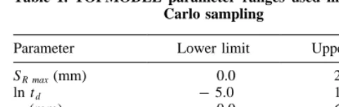
A Monte Carlo procedure was used to generate a large (104) number of sets of parameters for TOPMODEL, each para-meter value being drawn within ranges (see Table 1) thought feasible for the Minifelt on the basis of previous experience.19,21 Simulations were performed for each parameter set for comparison with the following sets of observations:
1. hourly flows measured during a 900-h period, October to November 1987;
2. hourly flows measured during a 600-h period, April 1989;
3. hourly water levels in four boreholes (labelled 4, 5, 6 and 7 in Fig. 1) for each of the two periods;
4. water levels in 108 piezometers, measured on three occasions, when the discharge at the outlet, averaged over measurement periods of less than 1 hour, was 0.1 mm h¹1, 0.61 mm h¹1or 6.8 mm h¹1.
For the flow and borehole simulations, the two observa-tion periods were modelled separately, i.e. TOPMODEL was re-initialised for the second period. Distributed piezo-meter water levels were simulated by direct application of the saturated zone formulation (eqns (1)–(4)), under an assumption that the discharge for each set of water levels corresponded to QSZin eqn (2). Values of ln(a/tanb) were
obtained for each piezometer location by linear interpola-tion within a gridded map.
Although interpolation allows point values of ln(a/tanb) to be estimated for each piezometer, these estimates never-theless reflect, to some degree, the grid-averaged nature of the topographic index distribution as calculated using a gridded DTM. This can be illustrated simply by considering the effect on point estimates of ln(a/tanb) of calculations based on different DTM grid resolutions; different interpo-lated values would be expected at any given point for dif-ferent grid element sizes. Point estimates of the topographic index are therefore somewhat uncertain for methodological reasons. Additionally, uncertainty may arise due to the highly simplified assumptions underlying the topographic index. Calculated values of ln(a/tanb) are constant over time and defined on a regular grid, in contrast to the real processes and soil properties that control local water table depths.
The TOPMODEL parameter space was explored by drawing parameter values randomly from uniform distribu-tions. This sampling method may be interpreted as reflecting ignorance about the prior marginal probability distributions of the TOPMODEL parameters over the ranges thought feasible. Such use of uniform prior distributions to represent a position of ignorance has been criticised in the context of the GLUE method by Clarke8(a general discussion may be found in Cox and Hinkley9). Given a deterministic model
Table 1. TOPMODEL parameter ranges used in the Monte Carlo sampling
Parameter Lower limit Upper limit
SR max(mm) 0.0 20.0
ln td ¹5.0 10.0
m (mm) 0.0 60.0
ln T0 ¹5.0 5.0
that has physically-meaningful parameters, it is possible that measurements could be used to define empirical prior dis-tributions. Although statistically appealing, this approach could risk over-interpretation of the physical significance of the model parameters, which are often defined in hydro-logical models at different scales than those at which suitable physical properties are measured.3,15 In the case of TOPMODEL, the exponential saturated zone store is areally integrated, as are flows at the outlet, allowing estimation of the value of the store parameter m directly from flow recession curve data.20However, in the following analysis, m was treated as if its value could not be deter-mined a priori. It will become apparent that there may still be uncertainty about the m parameter, especially when simulations of variables other than streamflow are considered.
4.2 Definition of the likelihood measure
In practice, the choice of parameter sampling distribution may not be critical since the prior distributions can be mod-ified by comparison of simulated data with observations, and this comparison is applied to complete sets of model parameters. A likelihood measure, L, is used to make the comparison, where, as noted above, the term ‘likelihood’ is interpreted fairly broadly to indicate goodness-of-fit. The measure chosen for this study was
L¼exp ¹Wj where W is a weighting factor, to be discussed below, j2e
is the variance of the simulation errors and j2o the
variance of the observed data. The function L would equal unity if the observed and simulated data were the same and reduces towards zero as the similarity decreases.
4.3 Rejection of non-behavioral simulations
There may be many parameter sets that lead to acceptable simulations of a given set of observations. Definitions of acceptability may vary according to context. For example, if a hydrological model is evaluated in terms of some simple goodness-of-fit function, less good values of this function may be considered acceptable for simulations of a time period known to pose particular difficulties for the model.
Allowance can be made within GLUE for the explicit definition of acceptability by the rejection of simulations for which the likelihood measure falls below a chosen threshold. The use of a rejection threshold is similar in approach to the Generalised Sensitivity Analysis (GSA) procedure of Spear and Hornberger28which divides multi-ple model simulations into a set that are judged to reproduce the behavior of the system and a set that are rejected as ‘non-behavioral’.
Previous application of TOPMODEL to the Minifelt19,21 suggested that very different values would be expected for the chosen goodness-of-fit measure (eqn (5)) when evaluated for simulations of discharge and water level data, leading to difficulties in the specification of a consistent rejection threshold. As a response to this, the approach of Binley and Beven7has been followed, where model simulations were ranked according to the likelihood measure and only the best 10% retained as ‘behavioral’.
It is recognised that the choice of a ‘best 10%’ rule to reject relatively poor simulations is somewhat arbitrary, and that the definition of the rejection rule may affect the uncer-tainty bounds computed using the GLUE method. In fact, tests demonstrated that relaxation of the rejection threshold to define a larger proportion of the total number of simula-tions as ‘behavioural’ would cause only slight modificasimula-tions of uncertainty bounds. The reason for this lack of great sensitivity to the rejection rule is that although the best parameter sets achieved values of L (conditioned on flow data) of 0.8, the majority of simulations achieved only extremely small values, particularly when conditioned on a combination of observed variables. Therefore, even if a larger number of parameter sets were retained as ‘beha-vioural’, predictions associated with many of the retained parameter sets would fall within the tails of the cumulative distributions of L and have little effect on the location of uncertainty bounds, computed according to the method described below.
4.4 Construction of uncertainty bounds
Simulation uncertainty bounds may be estimated from the parameter sets retained as behavioral by ranking the values of the simulation variable at the ordinate of interest (e.g. discharges at a given time step) and forming a cumulative distribution of corresponding values of the likelihood measure. Uncertainty bounds are then drawn at the values of the simulation variable that correspond to selected per-centiles of the cumulative likelihood distribution, in this study 5% and 95%.
It is worth emphasising that, although the uncertainty bounds are calculated at each ordinate, the likelihood measure is always evaluated over a whole simulation. The likelihood measure implicitly accounts14for any correlation in the marginal distributions of the parameters by taking a similar value for different parameter combinations that reflect such correlation.
4.5 Updating likelihood distributions
in the form
single set,Qi, of TOPMODEL parameters conditioned on two sets of observations Y1 and Y2, L(QilY1) is a prior
value, conditioned on the first set of observations Y1, L(QilY2) is evaluated with the new observations Y2, and C¼XL(QilY1,2). Eqn (6) was first applied to ‘update’
the likelihoods conditioned on the 1987 flow data with borehole water level observations from the 1987 period, rather than with a second period of flow data.
Repeated application of eqns (5) and (6) leads to an expression for the likelihood measure conditioned on n sets of observations, such that
L QilY1, …,n
Note that the use of an exponential function, such as eqn (5), in eqn (6) implies additive combination of the individual error variance terms within the exponent, allowing the weight given to the ith set of observations to be controlled by choosing a value for Wi. This is an important feature of
eqn (7) ifQisuccessfully reproduces some sets of observa-tions but gives rise to very poor simulaobserva-tions of other data; it may be undesirable in this case to rejectQi, but this would
happen if the individual variance ratios were multiplied directly.
In the results to be presented below, values of Wiwere
chosen for each period to give equal weight to errors from
the simulation of each individual set of borehole water levels and to share weighting equally between the combined error in simulations of all four boreholes and the errors in simulation of the flow data. When observations from the 1987 and 1989 periods were combined, equal weight was given to the simulation errors for each period. An exception to this scheme was made for the 1987 water level data from borehole 7, which were known to be inaccurate and for which the errors were given a weight of zero when combin-ing different borehole data sets uscombin-ing eqn (7). The values chosen for Wiin eqn (7) are given as a proportion of the sum
of weights in Table 2. The weighting of the distributed piezometer data will be discussed later.
5 RESULTS
5.1 Simulation uncertainties conditioned on a single period of discharge and borehole water level observations
Initially, simulations of the autumn 1987 flow data were compared with observations using the likelihood measure,
L (eqn (5)), and the best 10% (1000) simulations retained.
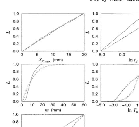
Cumulative distributions of L are shown in Fig. 2 for the five TOPMODEL parameters. The solid cumulative curves represent the posterior distributions of the parameters inferred from L, conditional upon the observed flow data. The uniform random sampling strategy, used to generate parameter values across the ranges shown, is equivalent to assuming the same value of any likelihood measure for every parameter set, prior to comparison between the associated simulations and the observed data. These prior distributions would appear in Fig. 2 as straight lines, plotted from lower left to upper right for each parameter. Deviations from such a line, seen in Fig. 2, indicate that conditioning on the observed flow data and retaining the best 1000 simula-tions has modified the prior position of ignorance about the TOPMODEL parameters, except for SR max and dv. The
strongest modification is suggested for the saturated zone parameters, m and lnT0.
These results are consistent with experience of the calibration of TOPMODEL, where simulated flows are gen-erally most sensitive to the values taken by m and lnT0. In
the relatively short period considered here, the unsaturated
Fig. 2. Rescaled distributions of the likelihood measure L for
TOPMODEL parameters, conditional on observations from the autumn 1987 period (tdin h m
¹1
, T0in m 2
h¹1).
Table 2. Proportional weights applied in eqn (7) to errors in evaluating combined likelihoods for different sets of
observations
Total time series 1 1
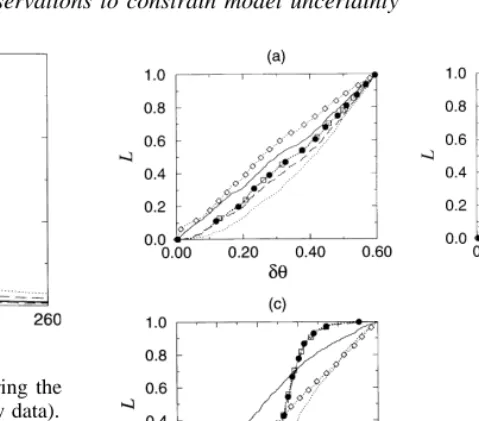
Fig. 3. (a) Uncertainty bounds computed for the first 300 h of the 1987 period (likelihood measure distributions conditioned on observations
from the whole 1987 period).
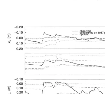
Fig. 4. (a) Uncertainty bounds for the main event in the 1989 period, showing the effect of updating ‘prior’ likelihood measure distributions
conditioned on flows from the 1987 period with the 1989 period flow data.
Fig. 4. (b) Prior and updated uncertainty bounds for borehole water levels for the 1989 period (note that the time axis corresponds to that in
zone parameters SR maxand tdwere unlikely to have as great
an effect on the simulated flow data. The posterior distribu-tion fordv is essentially the same as the prior distribution because the value taken bydvhas no effect on the simulated
flows.
The distributions of L were revised by applying eqn (7) to incorporate errors from the simulation of water levels recorded in the four boreholes during the 1987 period. Re-scaled cumulative distributions (dashed curves) are shown in Fig. 2, as are a set of distributions conditioned
only on the borehole water level observations (dotted
curves). The revised distributions, combining discharge and water level data, differ from the distributions condi-tioned on flow data alone. The main differences are that wider ranges of m and lnT0 appear to be able to explain
the combined sets of observations, some modification of the distribution for dv is seen, and the unsaturated zone parameters revert almost to uniform distributions.
These updated distributions suggest that observations of water level data have not helped to constrain the likely values of the TOPMODEL parameters, but have instead increased the uncertainty about these values. In the case ofdv, it is interesting that there has been relatively little refinement of the uniform prior distribution. This may be a result of the interaction between parameters; althoughdv
has no effect on simulated flows, m and lnT0 do have an
effect on simulated water levels.
Fig. 3(a) shows flow data from part of the autumn 1987 observation period plotted with two sets of computed uncer-tainty bounds or prediction intervals, the first conditioned on the observed flows alone and the second after the borehole water levels were brought into the likelihood measure. Both pairs of bounds enclose the observations, which is desirable. However, both lower bounds indicate very low flows for most of the period, and the simulation uncertainty is wide for the main storm event. The uncertainty bounds condi-tioned upon flows and water levels are wider than those conditioned on flows alone, especially for the first signifi-cant peak in the hydrograph. It is important to note that because the likelihood measure is calculated for an entire simulation, but uncertainty bounds are computed at every time step, the plotted bounds do not follow any one particular simulation. Thus, although the lower bounds in Fig. 3(a) are relatively flat, individual simulations can be much more dynamic.
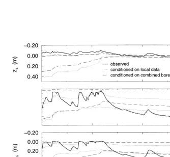
Simulation uncertainties are shown for the 1987 water level data in Fig. 3(b), which includes a dry period not shown in Fig. 3(a). Each set of borehole observations is plotted along with uncertainty bounds conditioned on the water levels recorded in that borehole (labelled ‘conditioned on local data’) and with a pair of bounds computed after combining the simulation errors from boreholes 4, 5 and 6 in eqn (7) (note again that the information from borehole 7 was given zero weight due to the unreliability of the data). The water level uncertainty bounds are less variable than the flow bounds of Fig. 3(a). Recessions are not well defined by the uncertainty bounds, which fail to enclose the
observed levels during the drier period. The deep lower bounds at the start of the period suggest that for some para-meter sets, the stores in TOPMODEL were not properly initialised (even though an initialisation period of 100 h was allowed). Borehole uncertainty bounds conditioned on a combination of flow and water level data are not shown, but do not differ greatly from the bounds conditioned on the combined borehole data.
The observed water levels in each borehole are better reflected by the bounds conditioned on observations in that borehole alone, in the sense that the these bounds tend to be narrower, indicate more dynamic responses and enclose the observations for nearly as much of the time as do the bounds computed using data from the combination of boreholes. This is important because of the implication that knowledge of water levels in several boreholes increases the uncertainty in simulations at one given location. Inspection of the observed water levels shows behaviour inconsistent with the simple assumptions of spatial uniformity in TOP-MODEL. The ponding of water on the surface at borehole 4 is notable, whilst there are slight differences in the timing of water level responses. Given the simple representation of processes in the model, the extent of the uncertainty shown in Fig. 3(b) seems realistic, as does the increase in uncer-tainty when observations from several boreholes are considered.
5.2 Updating uncertainty bounds with a second observation period
The likelihood measures computed in the previous section were used to plot uncertainty bounds for simulations of a second observation period, spring 1989. This may be inter-preted as using the distributions of the likelihood measure, evaluated with knowledge of the 1987 period observations, as prior likelihoods for simulation of the 1989 period. Within an optimisation framework, where only a single parameter set or simulation is retained, the procedure would be equivalent to model validation.
Discharge uncertainty bounds conditioned on the 1987 period flow data are shown in Fig. 4(a) for an event from the 1989 period. Also shown are bounds obtained after updating the likelihood measure by taking account of the flow data from the entire 1989 period. This was done with equal weight being given in eqn (7) to the error variances from each period. Qualitatively, both sets of bounds are similar to those computed for the 1987 period (Fig. 3(a)). Some reduction of the simulation uncertainty is seen after updating, mainly because of modification of the lower uncertainty bound. In contrast, for a combination of water level observations with flows in the likelihood measure, simulation uncertainty for discharge increased when data from the 1989 period were added. For clarity in Fig. 4(a), the resulting bounds are not shown, but were wider than those conditioned on flow data alone.
These bounds were computed for each borehole using like-lihoods conditioned by observations from that borehole only. One set of bounds was computed in each case using likelihood weights evaluated over the 1987 period as prior weights for the 1989 period. The second set of bounds show the effects of updating the likelihood weights with data from the 1989 period, which reduces the simulation uncertainty in each case. As for the 1987 period, the bounds do not enclose all of the observations, nor are the changes in water level tracked in any detail by either upper or lower bounds.
The updated likelihood distributions, conditioned on both 1987 and 1989 observation periods, also allow uncertainty bounds for the earlier period to be revised in light of the additional data. Revised estimates of simulation uncertainty for discharge during the main event in the 1987 period are shown in Fig. 5, conditioned on discharge data only. Information in the second period of observed flow data clearly causes the uncertainty bounds to change, shifting the range of likely model simulations to higher flow rates and reducing the extent of the uncertainty about the recession curve. The shift towards higher flows in both upper and lower updated bounds is due to greater likelihood being given to negative values of lnT0 in the updated parameter distribution, shown in Fig. 6(c) and labelled ‘FLOW’. This means that a relatively large proportion of the simulations used to compute the revised uncertainty bounds in Fig. 5 will have been associated with low satu-rated transmissivities, which tend to lead to the generation of rapid storm runoff, and hence high flow predictions, in TOPMODEL.
5.3 Incorporation of spatially-distributed water table observations in estimates of simulation uncertainty
Distributed water levels were simulated for comparison with the piezometer observations by the application of eqn (1) for each piezometer location. S was calculated¯
using eqn (2) and the saturated zone discharge QSZ was
assumed to be the flow observed at the time the water level observations were made. This assumption is only an approximation because saturated conditions were observed at some piezometers, implying that a component of the
discharge may have originated directly from coincident rainfall, rather than drainage of the saturated zone store. The approximation has been justified21 on the basis that measurements were taken during flow recessions and that the observed saturated areas were mainly due to return flow processes, which are implicit in the saturated zone storage relationship (eqn (2)). However, when simulating the distributed data, only the subsurface observations were considered, as the simple TOPMODEL structure used in this study could not be expected to represent in detail the complex transition as the water table rises above the surface through vegetation and organic litter and ponds in sub-grid scale topographic depressions.
Each set of water table observations was included in the likelihood measure with a weight Wi proportional to
the number of subsurface observations. Distributions of the likelihood measure conditioned on all available time series (flow and water level) data were then updated with the combined piezometer simulation errors, equal weight being given to the time series and the piezometer data.
Fig. 6 shows the posterior parameter distributions for the TOPMODEL saturated zone parameters conditioned on various combinations of observed variables, including a combination of discharges (FLOW), borehole time series (BH) and piezometer water levels (WT). It is notable that there has generally been relatively little refinement of the uniform prior distribution for the effective porosity, dv
(Fig. 6(a)). For m (Fig. 6(b)) there has been modification of the prior distribution as different sets of observations were considered. Uncertainty about m has been progres-sively constrained by knowledge of the piezometer water levels (marked ‘WT’), the borehole water levels (marked ‘BH’) and the flow data. The finding that flows (considered alone) bring about the greatest reduction in the likely range
Fig. 5. Prior and updated bounds for simulated flows during the
main storm event in the 1987 period (conditioned on flow data).
Fig. 6. Posterior distributions of the likelihood measure fordv(a), m (b) and ln T0(c) after conditioning using observations from both
periods. ‘BH’ indicates conditioned on borehole water levels, ‘WT’ indicates conditioned on piezometer water table data.
for m is reasonable, since m can theoretically be estimated directly (albeit with some uncertainty) from flow data by recession curve analysis.1,20
The distributions of the likelihood measure for lnT0
(Fig. 6(c)) fall into two groups, those where the logged borehole water level data were used and those conditioned only on flows or the piezometer water table data. The poster-ior distribution conditioned on flows from both periods is relatively uniform, and may be compared with the more constrained distribution when only the 1987 period was considered (Fig. 2). The distributed piezometer water table observations have also given rise to an almost uniform posterior distribution, but of reduced range. However, the greatest modifications of the uniform prior distribution have occurred through incorporation of the borehole water levels in the likelihood measure. Even when accorded only one quarter of the total weighting within eqn (7) (in combination with flow and piezometer data), it appears that the borehole observations are the dominant control on the posterior distribution of lnT0.
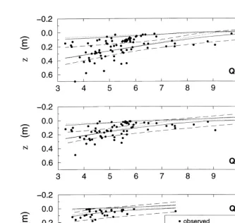
Fig. 7 shows uncertainty bounds for the simulation of the piezometer water table depths. These data are plotted with respect to the value of the topographic index, ln(a=tanb), at each location. This simplified presentation, plotting the data independently of physical location, is appropriate because the same prediction will be made by TOPMODEL for every point in the catchment having a given value of ln(a=tanb).
From eqn (1), when coupled with a linear scaling such as eqn (4), it follows that the simulated water table depths for any one set of model parameters would plot as straight lines in Fig. 7. It is clear that the observations are not consistent with such a simple model.
Errors in simulations of the water table depths generated by a single parameter set have been interpreted21in terms of variations in local values of the soil transmissivity that would be required to correct the simulated water table depths. These apparent local transmissivity values exhibited some relationship with ln(a=tanb), implying systematic errors in the index. However, there were considerable var-iations in the apparent transmissivities surrounding these trends, reflecting heterogeneity in the soil. Given the simple model structure tested here, it is a realistic response to the errors in water table predictions to express model output in terms of simulation uncertainties.
The uncertainty bounds in Fig. 7 were first computed using likelihoods conditioned on the time series data (combining flow and borehole data from both observation periods). Bounds were also computed from likelihood dis-tributions conditioned on the piezometer observations alone (but combining all three sets of measurements) and then on a combination of the piezometer observations with the time series data. Each pair of uncertainty bounds encloses some of the observations and indicates the expected tendency for TOPMODEL to predict smaller depths to the water table for
higher values of ln(a=tanb). The degree of uncertainty seems
consistent with the estimates for the borehole water levels, but many of the observed depths fall outside the calculated bounds, especially for the two lower discharges.
The main effects on the water table uncertainty bounds of incorporating the available time series observations within the likelihood measure are, firstly, a general tendency to shallower simulations and, secondly, a reduction in simula-tion uncertainty for higher ln(a=tanb)values. It is important to note that this reduction in simulation uncertainty does not imply that knowledge of the time series data necessarily improves the simulation of the distributed water table depths. In fact, the narrowing of the uncertainty in Fig. 7 causes many of the observed data to fall outside the computed bounds (see discussion below).
6 DISCUSSION
The results shown in Fig. 3(a) and Fig. 6 suggest that field observations of water levels, both in the form of time series at a limited number of point locations and more fully-distributed, but transient, measurements, have not greatly modified estimated simulation uncertainty for flows at the outlet of the Minifelt catchment. However, there are notable qualitative differences between the uncertainty bounds cal-culated for flow simulations and those calcal-culated for water level simulations. The uncertainty bounds for simulated borehole water levels shown in Fig. 3(b) and Fig. 4(b) do not vary greatly over time, in contrast to the observations. Although the uncertainty bounds generally enclose the logged borehole observations, this is merely because the bounds are relatively wide at all times, rather than following the observed data closely. This is in contrast to the uncer-tainty bounds calculated for flow simulations, where the value of the upper bound generally varies quite closely with the observed flows, and, given sufficient data, the lower flow bound also indicates responses to rainfall (see Fig. 4(a) and Fig. 5).
The borehole uncertainty bounds show little variation over time even when the likelihood measure, L, was condi-tioned solely on the ‘local’ data from a given borehole. However, single parameter sets can be found21to simulate reasonably well the variation of water levels, at least in boreholes 5 and 6, suggesting that the unresponsive borehole uncertainty bounds are not only due to the simplified representation of saturated zone dynamics in TOPMODEL. Indeed, whilst TOPMODEL might not repro-duce fully the propagation of water table fluctuations over very short time scales, water level changes can be simulated reasonably well at an hourly time step at single locations within shallow soils.21,26
Why, then, should the uncertainty bounds be wide and vary so little when individual simulations do show far more dynamic, realistic behavior? Considering evalua-tions of the likelihood measure conditioned on the combined borehole observations, an immediate reason
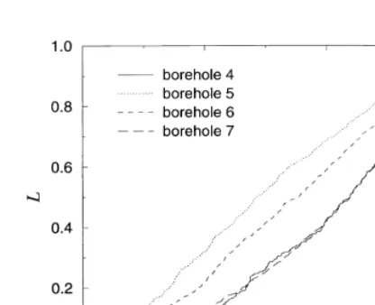
is found in the distributions of the likelihood measure for parameters lnT0 and dv, shown in Fig. 2. These
dis-tributions indicate that values of dv anywhere between 0.01 and 0.6 have been accorded similar likelihoods in the best 10% of the sampled parameter sets. Distributions conditioned separately on the individual boreholes were found to give a similar result in each case, as shown in Fig. 8. Combined with the constrained likely range for lnT0, seen in Fig. 6, the uncertainty about the value of dv
is reflected in wide borehole uncertainty bounds.
The lack of refinement of the prior uniform distribution for dv is surprising, given that this parameter directly influences the simulated water level through eqn (4). It has to be inferred that the relative insensitivity of the like-lihood measure todvfor any individual borehole is due to the interaction between dv, m and lnT0. Furthermore, the
highly simplified nature of the model cannot reproduce the effects of spatial variations in the soil, a factor which must lead to increased uncertainty when taking account of the observations from all four boreholes. This simplification is also apparent in the wide uncertainty bounds calculated for simulations of the piezometer data.
The wide uncertainty indicated for simulated water table depths is not surprising. The few studies that have attempted to relate values of ln(a=tanb)to measured water table depths have reported difficulties, with the easiest interpretation being that a distributed soils component or empirical correc-tion factor needs to be incorporated in the topographic index.18,21,26 Such an approach, based on modification of the topographic index, implies an argument that the basic TOPMODEL theory may be adequate for distributed pre-diction, but requires extra parameterisation to allow for local variations in soil properties. One way to introduce this local parameterisation may be the soils-topographic index, ln(a=T0tanb), which allows local saturated
transmissivity to vary in space.2
The results presented above for the current formulation of TOPMODEL, with soil properties treated as spatially-averaged, show ‘90%’ simulation uncertainty bounds that fail to enclose as many as 50% of the observed piezometer water level data (Fig. 7). What are the implications of these results? It should first be emphasised that these uncertainty bounds do not have the same meaning as confidence limits containing a fixed proportion of predictions, and which are drawn under assumptions about the distribution of predic-tion errors at each ordinate. Instead, the uncertainty bounds represent estimates, computed at each ordinate, of the range of predictions corresponding to a fixed proportion of the cumulative value of the likelihood measure associated with each parameter set or simulation. No assumptions are made about the nature of the distribution of prediction errors around the variable of interest.
in Fig. 7. However, such action would not improve the model predictions in any real sense. Instead, improvements to the model structure may have to be considered.
This is not to say that the model rejection rule and likelihood measure used here will always be the most appro-priate. Indeed, these methodological choices may be guided by trial-and-error. Although subjective, the choices made in applying the GLUE method are not entirely arbitrary, in the sense that a reasonable scientist will make reasonable and common sense choices. Here, the choices of likelihood measure and rejection threshold have been applied consis-tently using different sets of observations, and qualitative differences have emerged between the results obtained for predictions of flows, water level time series and distributed water table depths.
7 CONCLUSIONS
Measured depths to the water table have been used within a Bayesian procedure (GLUE) to evaluate simulation uncertainties for a simple version of the distributed rainfall–runoff model TOPMODEL. The water table data included both continuous, hourly measurements in four boreholes at different locations and observations from a network of piezometers, located throughout the catchment. Uncertainty bounds were computed for simulations of a period of measured flows and found to enclose the observations, although the lower bound often indicated the possibility of simulated flows being very low. When the continuous water level data from the four boreholes were given the same weight as the flow data in calculating uncertainty bounds, overall simulation uncertainty for discharges appeared to increase slightly.
Uncertainty bounds for the water levels in each borehole were found to be relatively wide and invariant over time. Combining observations from all four borehole locations led to greater uncertainty in water level simulations at any one location. Uncertainty in the case of individual boreholes
may be due in part to interaction between model parameters leading to equifinality between parameter sets and, conse-quently, little modification of a prior uniform distribution for parameterdv. The increased uncertainty after combining borehole observations from different locations is consistent with the simplification of spatial processes in TOPMODEL. The addition of a second observation period was found to modify uncertainty bounds for both flow and borehole water levels, causing lower flow bounds to follow the observations more closely, but not always decreasing the uncertainty, nor improving qualitatively the borehole water level bounds.
Spatially distributed simulation uncertainties were also estimated using water table depths, measured throughout the Minifelt catchment. These data were found to have relatively little effect on parameter distributions conditioned on observed flows and continuous water levels in the four boreholes. Data from the four logged boreholes appeared to be dominant in determining posterior distributions of the TOPMODEL parameters. One conclusion to be drawn from this result is that continuous water table observations from a few locations may be as useful as an extensive set of transient water table measurements in constraining the uncertainty of the parameters in TOPMODEL, although this is not to say that extensive water table data are of less value in other regards. For simulations of water table depths at each piezometer, differences were found between uncertainty bounds conditioned solely on flow and borehole data and bounds also taking the piezometer data into account.
This study is a first attempt to test simulations of extensive, spatially distributed water table measurements within the GLUE framework. The failure of the simulation uncertainty bounds to enclose many of the observed water table depths does not necessarily lead to outright rejection of the hydrological model, but draws attention to its limita-tions, in particular the adequacy of the topographic index ln(a=tanb)as a predictor of water table position when soil properties are assumed to be uniform.
Can better results be obtained, within the uncertainty framework, using a modified formulation of TOPMODEL, or any other distributed hydrological model? We feel that many of the implications of this study will be generic to distributed models, regardless of whether they are more or less physically-based. Even a ‘physically correct’ model cannot be applied using local effective parameters ubiqui-tously, as techniques for measuring or estimating effective values at model grid scales do not exist. This will inevitably lead to errors in local predictions.
Any attempt to condition spatially-distributed parameters using comparisons between predictions and observations is likely to face the problems of parameter interactions and equifinality, incidentally limiting the number of parameters that can reasonably be estimated. Predictive uncertainty can be expected as a result of these problems. However, it is not yet clear what the limits of predictability might be for distributed hydrological models.
ACKNOWLEDGEMENTS
This work was funded by NERC grant GT4/92/192/P. The Minifelt field study was supported by the Norwegian National Committee for Hydrology (NHK) and the Norwegian Research Council. Peter Troch and two anonymous referees are thanked for their helpful comments.
REFERENCES
1. Beven, K. and Kirkby, M. J. A physically based, variable contributing area model of basin hydrology. Hydrological Sciences Bulletin, 1979, 24, 43–69.
2. Beven, K., Hillslope runoff processes and flood frequency characteristics. In Hillslope Processes, ed. A. D. Abrahams. Allen and Unwin, Boston, 1986, pp. 187–202.
3. Beven, K. Changing ideas in hydrology: The case of physically-based models. Journal of Hydrology, 1989, 105, 157–172.
4. Beven, K. and Binley, A. The future of distributed models— model calibration and uncertainty prediction. Hydrological Processes, 1992, 6, 279–298.
5. Beven, K. Prophecy, reality and uncertainty in distributed hydrological modelling. Advances in Water Resources, 1993, 16, 41–51.
6. Beven, K., Lamb, R., Quinn, P., Romanowicz, R. and Freer, J., TOPMODEL. In Computer Models of Watershed Hydrol-ogy, ed. V. P. Singh. Water Resources Publications, Color-ado, 1995, pp. 627–668.
7. Binley, A. and Beven, K., Physically-based modelling of catchment hydrology: a likelihood approach to reducing pre-dictive uncertainty. In Computer Modelling in the Environ-mental Sciences, ed. D. G. Farmer and M. J. Rycroft. The Institute of Mathematics and its Applications Conference Series, Clarendon Press, Oxford, 1991, pp. 75–88.
8. Clarke, R., Statistical Modelling In Hydrology. John Wiley and Sons, Chichester, 1994.
9. Cox, D. R. and Hinkley, D. V., Theoretical Statistics. Chapman and Hall, London, 1974.
10. Duan, Q. S., Sorooshian, S. and Gupta, V. K. Effective and efficient global optimisation for conceptual rainfall–runoff models. Water Resources Research, 1992, 28, 1015–1031. 11. Dunne, T., Field studies of hillslope flow processes. In
Hill-slope Hydrology, ed. M. J. Kirkby. John Wiley and Sons, Chichester, 1978, pp. 227–293.
12. Erichsen, B. and Myrabø, S., Studies of the relationship between soil moisture and topography in a small catchment. In Proc. 8th International Conference on Computational Methods in Water Resources, ed. G. Gambolati, Computa-tional Mechanics Publications, Southampton, 1990. 13. Franks, S., Beven, K. J. and Lamb, R., Assessing the utility of
distributed data in constraining the behaviour of hydrological models in the Wijlegemse subcatchment. In Spatial and
temporal soil moisture mapping from ERS-1 and JERS-1 SAR data and macroscale hydrological modelling, ed. F. P. De Troch, P. A. Troch and Z. Su. Final Research Report, EC Environment Research Program EV5V-CT94-0446, Gent, Belgium, 1997, pp. 334–357.
14. Freer, J., Beven, K. and Ambroise, B. Bayesian estimation of uncertainty in runoff prediction and the value of data: An application of the GLUE approach. Water Resources Research, 1996, 32, 2161–2173.
15. Grayson, R. B., Moore, I. D. and McMahon, T. A. Physically-based hydrologic modelling. 2. Is the concept realistic?. Water Resources Research, 1992, 28, 2659. 16. Hewlett, J. D. and Hibbert, A. R., Factors affecting the
response of small watersheds to precipitation in humid areas. In Forest Hydrology, ed. W. E. Sopper and H. W. Lull. Pergamon, Oxford, 1967, pp. 275–290. 17. Hursh, C. R. and Brater, E. F. Separating storm-hydrographs
from small drainage-areas into surface- and subsurface-flow. Transactions, American Geophysical Union, 1941, 22, 863–870.
18. Jordan, J. P. Spatial and temporal variability of stormflow generation processes on a Swiss catchment. Journal of Hydrology, 1994, 153, 357–382.
19. Lamb, R., Distributed hydrological predictions using a gen-eralized TOPMODEL formulation. Ph.D. thesis, University of Lancaster, UK, 1996.
20. Lamb, R. and Beven, K. Using interactive recession curve analysis to specify a general catchment storage model. Hydrology and Earth System Sciences, 1997, 1, 101–113.
21. Lamb, R., Beven, K. and Myrabø, S. Discharge and water table predictions using a generalized TOPMODEL formula-tion. Hydrological Processes, 1997, 11, 1145–1167. 22. Myrabø, S. Automation in hillslope hydrology. NHP-rapport,
1988, 22, 36–45.
23. Myrabø, S. Temporal and spatial scale of response area and groundwater variation in till. Hydrological Processes, 1997,
11, 1861–1880.
24. Quinn, P. F., Beven, K. J. and Lamb, R. The ln(a/tanb) index: How to calculate it and how to use it within the TOPMODEL framework. Hydrological Processes, 1995, 9, 161–182. 25. Romanowicz, R., Beven, K. J. and Tawn, J. A., Evaluation of
predictive uncertainty in nonlinear hydrological models using a Bayesian approach. In Statistics for the Environment 2: Water Related Issues, ed. V. Barnett and K. Feridum-Turkman. Wiley, Chichester, 1994, pp. 297–317.
26. Seibert, J., Bishop, K. H. and Nyberg, L. A test of TOPMO-DEL’s ability to predict spatially distributed groundwater levels. Hydrological Processes, 1997, 11, 1131–1144. 27. Sorooshian, S. and Gupta, V. K. Automatic calibration of
conceptual rainfall–runoff models: the question of parameter observability and uniqueness. Water Resources Research, 1983, 19, 260–268.
28. Spear, R. C. and Hornberger, G. M. Eutrophication in Peel Inlet, II. Identification of critical uncertainties via General-ised Sensitivity Analysis. Water Resources Research, 1980,