Conference paper

EXPLOITING SATELLITE FOCAL PLANE GEOMETRY FOR AUTOMATIC

EXTRACTION OF TRAFFIC FLOW FROM SINGLE OPTICAL SATELLITE IMAGERY

Thomas Krauß

DLR – German Aerospace Center, Remote Sensing Institute, M¨unchener Str. 20, 82234 Oberpfaffenhofen, thomas.krauss@dlr.de

Commission I, WG I/4

KEY WORDS:Optical Satellite Data, Focal plane assembly, Traffic detection, Moving objects detection

ABSTRACT:

The focal plane assembly of most pushbroom scanner satellites is built up in a way that different multispectral or multispectral and panchromatic bands are not all acquired exactly at the same time. This effect is due to offsets of some millimeters of the CCD-lines in the focal plane. Exploiting this special configuration allows the detection of objects moving during this small time span. In this paper we present a method for automatic detection and extraction of moving objects – mainly traffic – from single very high resolution optical satellite imagery of different sensors. The sensors investigated are WorldView-2, RapidEye, Pl´eiades and also the new SkyBox satellites.

Different sensors require different approaches for detecting moving objects. Since the objects are mapped on different positions only in different spectral bands also the change of spectral properties have to be taken into account. In case the main distance in the focal plane is between the multispectral and the panchromatic CCD-line like for Pl´eiades an approach for weighted integration to receive mostly identical images is investigated. Other approaches for RapidEye and WorldView-2 are also shown. From these intermediate bands difference images are calculated and a method for detecting the moving objects from these difference images is proposed.

Based on these presented methods images from different sensors are processed and the results are assessed for detection quality – how many moving objects can be detected, how many are missed – and accuracy – how accurate is the derived speed and size of the objects. Finally the results are discussed and an outlook for possible improvements towards operational processing is presented.

1. INTRODUCTION

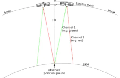
Actual very high resolution (VHR) satellite sensors are mostly operated as pushbroom scanners with different CCD-arrays for each panchromatic or multispectral band. If these arrays are moun-ted in distances of millimeters or even centimeters in the focal plane assembly (FPA) the same ground point is not acquired at the same time in all CCD-arrays. This principle is shown in fig. 1.

Figure 1: Principle of acquisition geometry of image bands sepa-rated in a FPA

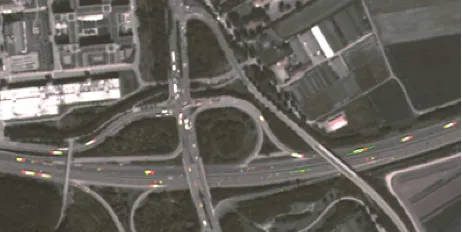
If moving objects are recorded by a sensor whith such an ac-quisition system the object appears in different positions at each band. See for an example fig. 2. This image shows a part of an RapidEye satellite scene containing a plane. The plane appears at different positions in the blue, green and red band.

In this work we will exploit this feature of many sensors to au-tomatically detect moving traffic in satellite images. The sensors

Figure 2: Section2.1×_{1.5km from a RapidEye scene of southern} bavaria (north of F¨ussen) containing clouds and a plane

investigated are WorldView-2, RapidEye, Pl´eiades and also the new SkyBox satellites.

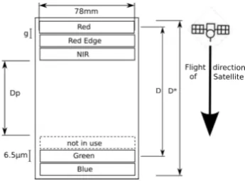
RapidEye there is a large gap in the size of several millimetres between the scan lines for red/red-edge/near-infrared (NIR) and green/blue but only about 6.5 micrometres inside the lines be-tween e.g. green and blue. This assembly results in the colored cyan/red corners which can be detected easily in each Rapid-Eye image containing clouds (see also fig. 2 for this effect). For WorldView-2 there exist two four-line multispectral CCD lines – one for the “classic” bands blue/green/red/NIR and one for extra bands coastal/yellow/red-edge/NIR2. Between these two four-channel-CCD-lines the panchromatic CCD-line is located. For Pl´eiades there exist one multispectral four-channel-CCD-line and one panchromatic CCD-line. In case of the SkyBox satellites the configuration is a little more complicated. SkyBox uses three frame sensors, each divided in a panchomatic part in the upper half and the four multispectral bands blue/green/red/NIR in the lower half of the frame. Operated in the scanning mode there is also a small time distance between each of the color bands and also to the panchromatic band.

First we present the design of the focal plane assembly (FPA) of each of the sensors to describe which bands are selected for the moving object detection. Second we describe the method for au-tomatically extraction of moving objects. Afterwards the method is applied to images of the different sensors and the results are shown and evaluated. Finally the method is assessed and an out-look for further improvements of the method is given.

But first let’s have a look on the focal plane assemblies, acquisi-tion principles and example imagery of our sensors.

2. ACQUISITION PRINCIPLES AND FOCAL PLANE ASSEMBLIES

2.1 WorldView-2

The WorldView-2 multispectral instrument consists of two mul-tispectral CCD lines acquiring in the first the standard channels blue, green, red and the first near infrared band and in the sec-ond the extended channels coastal blue, yellow, red edge and the second near infrared band. These two CCD lines are mounted on each side of the panchromatic CCD line. Therefore the same point on ground is acquired by each line at a different time. Fig. 3 shows the focal plane assembly (FPA) of WorldView-2.

Figure 3: Focal plane assemblies of WorldView-2 (sketch cour-tesy Digital Globe)

In table 1 from K¨a¨ab (2011) the time lags for the sensor bands are given.

In our investigations we use the yellow and red bands from MS2 and MS1 respectively due to the good spectral correlation for most traffic objects in this spectral range. The time difference ∆tW V2for these two bands corresponding to table 1 is0.340s−

0.016s= 0.324s which is in good correlation to our calibration results of∆tyr = 0.297±0.085s as derived in Krauß et al.

Table 1: WorldView-2’s recording properties Band recording Sensor Wavelength Inter-band Time lag [s] data order name [nm] Time lag [s] from start

Near-IR2 MS2 860-1040 Recording start Recording start Coastal Blue MS2 400-450 0.008 0.008

Yellow MS2 585-625 0.008 0.016

Red-Edge MS2 705-745 0.008 0.024

Panchromatic PAN 450-800

Blue MS1 450-510 0.3 0.324

Green MS1 510-580 0.008 0.332

Red MS1 630-690 0.008 0.340

Near-IR1 MS1 770-895 0.008 0.348

(2013). Fig. 4 shows a section (800×_{400m) of a WorldView-2} scene in the north of Munich (A99) consisting of the yellow and red band.

Figure 4: Displacement of cars seen by WorldView-2 in the red and yellow band (section800×_{400m on A99 north of Munich)}

In this image the displacement of moving cars in the two channels is clearly visible. Knowing the right-hand-traffic in Germany we see, the red band is acquired earlier than the yellow band and the image was acquired in forward direction. Fig. 5 shows the two profiles of a car (left, also left green profile-line in fig. 4) and a large truck (right).

Figure 5: Profiles of a car (left) and a truck (right); red channel shown in red, yellow channel in green

2.2 RapidEye

As shown in fig. 6 the RapidEye focal plane assembly consists of five separate CCD lines – one for each band. They are grouped in two mounts: the blue and green on one and the red, red edge and the near infrared band on the second.

Figure 6: RapidEye focal plane assembly (FPA),g: gap between lines,Dp: distance between packages,D∗: maximum distance between lines,D: distance red–green

Figure 7: Displacement of cars seen by RapidEye (in cyan/red, section900×_280m)

2.3 Pl´eiades

The Pl´eiades FPA is similar but consists only of one multispec-tral and one panchromatic sensor line. The main gap exists only between the multispectral bands and the pan channel where the latter is also mounted in a curvature around the optical distor-tion center (marked with a×_{in the figure) as shown in fig. 8.} Delvit et al. (2012) stated for the time difference between the multispectral and the PAN CCD∆tms,pan = 0.15s where we found in our previous calibration (Krauß et al., 2013) a value of ∆tms,pan= 0.16±0.06s.

Figure 8: Focal plane assembly Pl´eiades (curvature of PAN sen-sor strongly exaggerated)

In fig. 9 a section160×_{100m of the M1 in Melbourne near the} harbour is shown. The PAN channel in red, the combined multi-spectral channels in cyan. Since in Australia is left handed traffic the cars are travelling from left to right. So the PAN channel is acquired before the multispectral bands. In fig. 10 the two pro-files along the green lines in fig. 9 are shown. The left profile is the profile of the truck (left in fig. 9), the right profile the profile of the two cars on the right.

To combine the PAN and multispectral channels for a parallel processing the PAN channel has to be reduced in resolution and the multispectral bands have to be combined to a panchromatic band.

Figure 9: Example of a combined PAN (red) and multispectral (cyan) Pl´eiades image, section160×_{100m of the M1 in} Mel-bourne near the harbour.

Figure 10: Profiles along the green lines from fig. 9, left: truck (also left in image), right: two cars, all travelling from left to right, DN vs. metres

Using the spectral response function of the multispectral bands (weightswicorresponding to the part of the multispectral band contained in PAN channel) and taking into account the physical gainsgias listed in tab. 2 a synthetic panchromatic band can be calculated from the multispectral bandsMSias follows:

Pms=

4

X

i=1

wi·MSi·gi

gp·

4

X

i=1

wi

(1)

Table 2: Weights w and gainsg for the investigated Pl´eiades scene

Index Band Weightw Gaing

1 Blue 0.3 0.104275286757039 2 Green 1.0 0.109170305676856 3 Red 0.9 0.0968054211035818 4 NIR 0.5 0.0639386189258312

p PAN 2.7 0.0880281690140845

On the other hand the PAN channel has to be resampled correctly to the 4-times lower resolution multispectral bands. This can be achieved by scaling down the PAN channel using an area averag-ing and applyaverag-ing a gaussian filter withσ= 0.7px:

Ppan=γ0.7 scale1/4(P AN)

(2)

2.4 SkyBox

Figure 11: Focal plane assembly SkyBox, three frame cameras splitted in a PAN and four multispectral bands

Fig. 12 shows an example of a plane crossing the acquisition path of SkyBox. The image is a orthorectified composite of the 1-m-PAN-band (in gray) and overlayed the four 2.5-m-multispectral bands (blue, green, red and NIR shown as purple). As can easily be seen in the PAN band the image consists of about 20 single frame camera images which are merged to one master image in the SkyBox level-1B-preprocessing. The same procedure is ap-plied to the four half-resolution multispectral bands. But with the lower resolution no single planes will be visible here any more but only one blurred combined image. The distances of the centres of the plane images correlate with the FPA as shown in fig. 11.

Figure 12: Example of a Skybox image showing a moving plane in PAN, blue, green, red and NIR channel (2014-08-09, detector 3, image 6)

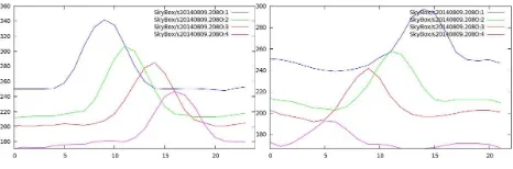
Fig. 13 shows a section of the N568 near Fos-sur-Mer (Camargue, France). Fig. 14 shows the two profiles marked in fig. 13, left the top, bright, right the lower, darker car.

The profiles are the 2.5 m multispectral image data resampled to the 1-m-PAN ortho-image. As can be seen, the cars – merged from four camera-frames – are shown as smooth curves. The maxima of each curve can be correlated to estimate the speed.

For SkyBox no calibration of the time gap∆texists until now. But from the NORAD two line elements (TLE) we can derive an average height ofhs = 581.5km above earth and an aver-age speed ofv= 7564.25m/s. This corresponds to an average ground speed of

vg = v ·_RE RE+hs

(3)

with an earth radius of 6371 kmvg become 6931.58 m/s. An original multispectral image with a nominal GSD of 2.39 m has

Figure 13: Skybox image showing the displacement of cars in the red, green and blue band, section620×_{750m, N568 near} Fos-sur-Mer (Camargue, France)

Figure 14: Profiles of two cars, left: top profile, right: lower pro-file from fig. 13, bands blue, green, red, NIR (as purple), digitial numbers (DN) vs. metres

540 rows or a length in flight direction ofl= 1290.6m. So the acquisition of this image needstms=l/vg = 0.186s.

2.5 Preliminary work

In a previous investigation (Krauß et al., 2013) we showed how to calibrate the time gaps∆tbetween different bands in single RapidEye and (multi-)stereo WorldView-2 and Pl´eiades images. The work was inspired in the detection of colored artifacts near moving objects.

Deeper analysis shows that this effect was already known from the first very high resolution (VHR) commercial satellites such as QuickBird and Ikonos. Etaya et al. (2004) uses already in 2004 QuickBird images of 0.6 m GSD panchromatic and 2.4 m multi-spectral and found a time gap between these bands of about 0.2 s. In the same way M. Pesaresi (2007) found also a time lag of 0.2 seconds between the panchromatic and the multispectral bands of QuickBird images.

In an IGARSS paper Tao and Yu (2011) proposed the usage of WorldView-2 imagery for tracking moving objects. He calculated from a plane arriving at the Shanghai airport a time delay between the Coastal Blue Band on the second multispectral sensor line and the Blue Band on the first multispectral sensor line of about 17.5 m/80 m/s = 0.216seconds.

using a matching accuracy of about 0.1 pixels allow for the ex-traction of a DEM with an uncertainty of 120 m (0.1×₄×_300m for the multispectral GSD pixel size).

Also Leitloff (2011) gives in his PHD thesis a short overview of more of these methods and proposed also some approaches for automatic vehicle extraction of still traffic.

But none of these investigations tried to do an automatic detection of traffic in whole very high resolution (VHR) satellite scenes. All of the previous researches show only the possibility and de-rive the time gaps. In our here presented work we propose dif-ferent methods tailored for the difdif-ferent sensors investigated to detect automatically some of the traffic in the imagery to derive traffic parameters like an average speed per road segment.

3. METHOD

As shown in the previous chapters all of the very high resolution (VHR) satellite sensors investigated in this paper allow the ex-traction of moving objects from only one single satellite image. This can be achieved by exploiting a small time gap∆tin the acquisition of different bands as summarized in tab. 3.

Table 3: Overview of time gaps and bands used for the investi-gated sensors

Sensor Bands ∆t[s] Resolution/GSD [m]

WorldView-2 yellow-red 0.324 2.0 RapidEye green-red 2.65±0.50 5.0 Pl´eiades MS-PAN 0.16±0.06 2.0 SkyBox green-red 0.186 _2.4

To correlate the needed bands they must have the same ground sampling distance (GSD) and should have the best possible sim-ilar spectral properties for the investigated objects. For traffic – cars and trucks – the red band and the nearest possible band with lower wavelength appeared to give the best correlations. So mostly in tab. 3 a red band together with a green or yellow band occur. The main exception is the Pl´eiades system where we have to create two synthetic low resolution panchromatic bands as ex-plained in eqs. 1 and 2.

To detect the moving objects in a first step difference images be-tween the above mentioned bands are created as shown in fig. 4. Fig. 15 shows the first step of the method where the bands in-volved are subtracted and the difference is median filtered with a merely large radius of about 18 m (9 pixels in the case of WorldView-2).

Figure 15: Sample processing of bands, step 1, example WorldView-2, left: difference image of red and yellow band, right: median filtered difference

Fig. 16 shows the second step of the object detection. Here the calculated median is subtracted from the difference image to em-phasize only small local differences. Afterwards these differ-ences are thresholded (1/6 of absolute brightness) and marked as positive or negative objects.

Figure 16: Sample processing of bands, step 2, example WorldView-2, left: difference image relative to median, right: de-tected positive and negative objects

In the third step the detected objects from fig. 16 (right) are fetched from the image and the nearest, best fitting (in sum of bright-nesses) objects are taken as the “from” and “to” car positions. Using the distance of the centers of gravity of these positions to-gether with the time gap∆tfor the bands of the sensor gives the speed of the object. Until now no restictions to road directions is included. So also a best match can be found across lanes.

4. EXPERIMENTS

4.1 WorldView-2

First we applied our method to a WorldView-2 dataset acquired on 2012-07-10 over Munich (Germany). Our method found 3615 objects in the whole area of16.4×_19.8km2

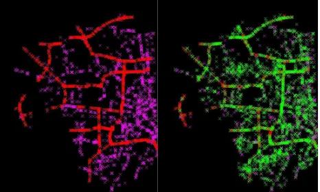
– mostly cars and trucks – in about 2 minutes. Two references where created manu-ally: one containing all moving cars and trucks on highways and main roads as shown in fig. 17 (left, in red) and one containing all other moving traffic on all other roads in the image (left, in purple). Fig. 17 (right) shows all automatically detected objects overlaid in green.

Figure 17: WorldView-2 scene, western half of Munich (16.4× 19.8 km2

), left: manually measured reference (cars on high-ways/main roads in red, all other cars in purple), right: automati-cally detected cars overlaid in green

In table 4 the results for the 3615 found objects against the manu-ally measured objects are listed. In total 2063 objects from 4020 reference objects or 51 % were detected correctly. But also a high rate of 1957 objects (49 %) was not detected. The wrongly de-tected 1552 objects (43 % of all dede-tected objects) can partly also be explained by missing objects in the manually measurement.

Table 4: Overview of time gaps and bands used for the investi-gated sensors

Objects Detected Detected Not Reference in reference correctly false detected

All 4020 2063 1552 1957

Highways/main roads 2312 1083 2532 1229

Other roads 1708 997 2618 711

objects show that some objects where detected by the automatic method which are existing but were just overseen by the manual measurements of about 6 students over 3 months.

Also a comparison of the detected speeds of the 3615 found ob-jects was performed. Therefore for 2312 cars from the above mentioned reference both positions in the yellow and red band were measured. Fig. 18 shows the difference object image with the found derived speeds as green arrows and the original yel-low/red bands with the manually measured objects as green crosses.

Figure 18: Correlation of measured vs. automatically detected speeds, left: difference object image, right: yellow/red image (in red/cyan), green crosses are the manual measurements of the from/to objects, the green arrows in the left image are the auto-matically derived speeds

The correlation of the automatically detected objects to these mea-sured speed reference was done by taking a correlation if both positions (in the red and yellow band) of the detected and the manually measured object lied inside a correlation radiusradof 3, 10 or 100 pixels.

Table 5: Accuracy assessment of detected speeds in the WorldView-2 scene

Detected Reversed Not Detected Mean speed Std. dev. rad correctly direction detected false ¯v[km/h] σv[km/h]

3 894 50 1418 2721 13.1974 24.4084

10 1067 238 1245 2548 24.5571 45.2691

30 1187 425 1125 2428 25.6629 46.7234

100 1377 707 935 2238 27.0640 49.1532

Table 5 shows the calculated results of the correlation of the au-tomatically detected to the manually measured objects together with the mean difference and standard deviation of the derived speeds. As can be seen more objects can be correlated between the automatic detected results and the manual measurement as the correlation radius increases. But also the mean speed difference and the standard deviation rises abruptly at a correlation radius higher than three pixels.

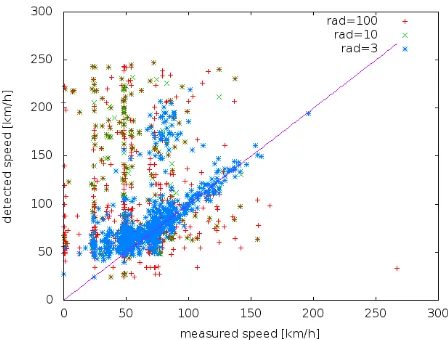
In fig. 19 the correlation of the detected objects is plotted for three correlation radii. As can be seen the blue points (correlation radius 3) fit already very good to the measurements. But between 50 and 100 km/h there can be found a bunch of outliers where the automatically derived speeds lie between 150 and 200 km/h. This is due to the missing correct detection of trucks in the images. Please refer for the explanation to the profiles shown in fig. 5 referring to the yellow-red-image in fig. 4.

Figure 19: Correlation of measured vs. automatically detected speeds (correlation radiusradin pixels of GSD 2 m)

The method just does a difference of the image values. In the left case of fig. 5 (a car) there remains a red and a yellow blob which are correlated correctly. But in the case of a truck (right profile) the difference splits up the object to a left and a right object since the center part of the truck vanishes in the difference. In this case correlating the two split up blobs of the truck gives a virtual speed depending on the real speed and the length of the truck. To solve this problem the method has to be expanded to detect trucks as continous objects before doing the correlation.

4.2 RapidEye

For assessing the method with a RapidEye scene we use a scene acquired 2011-04-08 from an area west of Munich containing the A96 and the lakes Ammersee and Starnberger See as shown in fig. 20. The results for a small section6×_2km2

with the A96 near Sch¨offelding are shown in fig. 21.

Figure 20: RapidEye Scene used for assesment, west of Munich, 100×₁₀₀km2

driving with the same speed. A profile across these cars is shown in fig. 22.

Figure 21: Objects found in part RapidEye Scene,6×_2km2_, A96 near Sch¨offelding, green arrows denote movement of ob-jects, green line across cars in center for profile in fig. 22

Figure 22: Profile along green line of RapidEye scene in fig. 21, reflections×_{100in [%] vs. metres along road}

An assessment was made along a 15 km long strip of the A96. The results are shown in tab. 6. Along the highway 61 vehicles were manually detected, 81 were detected by the presented auto-matic method. From these 46 where found erroneously (mostly in clouds) and 21 manually marked objects were missed – mostly due to the too bad contrast. 21 objects were detected correctly whereas 14 detected objects were detected but correlated with the wrong mate in the other band. Typical errors can be seen in fig. 23.

Table 6: Accuracy assessment of detected objects along a 15 km strip of the A96

81 Detected in total 61 Reference 21 Detected correctly

14 Detected, but correlated wrong 26 Not detected (mostly too bad contrast) 46 Detected erroneous (mostly clouds)

4.3 Pl´eiades

For assessing our algorithm with the Pl´eiades sensor we used a scene acquired 2012-02-25 over Melbourne, Australia. As shown in fig. 24 we evaluated the quality of our method on a4×_2km2 section of the harbour of Melbourne containing a strip of the M1 highway. Fig. 24 shows the 265 manually measured cars (and one ship, yellow crosses) together with all 300 automatically found objects (green crosses).

Applying the method to the Melbourne-harbour-image finds 300 moving objects. As shown in tab. 7 the quality is not so good. Only 115 of 265 objects were detected correctly which corre-sponds to a detection rate of only 43.4 %. In contrast 185 of the 300 detected objects were no moving objects (false detect rate of 61.7 %).

Figure 23: Typical errors in a RapidEye Scene, left on border: correctly detected car at cloud-border, left: erroneous detections in clouds, center: (single yellow cross) missed car due to bad contrast, right: wrong correlation of cars on opposite lanes

Figure 24: Example Pl´eiades image,4×_2km2

, harbour of Mel-bourne (Australia), top: reference of manually measured cars (yellow crosses), bottom: automatically found moving objects (green crosses)

As can be seen in fig. 24 these erroneously detected objects are located mostly in the top left of the scene where the oil terminal with many oiltanks and in the marina on the right center contain-ing many small ships. However also one ship (upper part, left of center) was found by the method even if the speed was absolutely overestimated with 139 km/h instead of 0.8 m/0.16 s or 18 km/h.

4.4 SkyBox

For assessing the SkyBox system an image from 2014-08-09 in the south of France near Fos-sur-Mer (Camargue, France) was available. In the orthorectified scene 8 of detector 2 (3×₂km2

) all moving objects were marked manually and automatically de-tected in 11 seconds as shown in fig. 25.

Assessment of the result vs. the manually measurement shows 21 automatically detected objects and 22 manually measured ob-jects. From these 12 were correct detected, 10 cars were missed and 9 objects – mostly in the industrial area in the bottom cen-ter of the image – were wrongly detected as moving object. So for SkyBox using the red and green band also a detection rate of 54.5 % and a false-detect-rate of 42.9 % can be found while no miscorrelations were found in the test scene.

5. RESULTS

Table 7: Pl´eiades accuracy assessment

Figure 25: Example SkyBox image, 3×_2km2 _near Fos-sur-Mer in southern France, top: reference of manually measured cars (yellow crosses), bottom: automatically found moving ob-jects (green crosses)

by all manually measured cars. The false-detect-rate is the num-ber of objects detected automatically but not manually verified divided by all automatically detected objects. The miscorrelation rate is the number of wrongly correlated objects divided by the number of all correctly detected objects (so the object was found correctly in one band, but the wrong mate in the other band was taken for the speed calculation).

Table 8: Quality measures for the assessed sensors Sensor Detection rate False-detect-rate Miscorrelation-rate

World-View-2 51.3 % 42.9 % 20.9 %

RapidEye 57.4 % 56.8 % 40.0 %

Pl´eiades 43.4 % 61.7 % 3.5 %

SkyBox 54.5 % 42.9 % 0.0 %

The missed objects (objects not detected, 100 %−_{“detection rate”)} are mostly due to too low contrast of the object relative to the road. So cars with the same color as the road cannot be de-tected. Also cars darker than the road are detected not so well. If a dark car with good contrast to the road is detected the presented method will give the wrong driving direction – but this happened only by investigating the WorldView-2 image and only in 5.6 % of all detected cars (“reversed direction” in tab. 5: 50/894). In the RapidEye image e.g. the image quality was too bad to detect dark

cars on the road.

The false-detect-rate mostly contains objects far away from streets with spectral signatures which look similar to those of moving objects. This rate may be reduced dramatically by introducing a road mask.

The miscorrelation is mostly based on better and nearer matches on neighbouring lanes as shown in fig. 23 (right). So this may be reduced also using the road mask and only allowing correlations along road directions.

With this presented method the Pl´eiades sensor perfom badest due to the very low time gap of only 0.16 s which results in large overlaps of also small moving objects. Consequently the derived speeds are mostly too high (even for cars!) if the objects have a remaining overlap in the two investigated bands. Additionally the channel merging method proposed for Pl´eiades in eqs. 1 and 2 give some artifacts on borders of buildings, ships and – as seen in the test area – oiltanks which result in a huge number of erro-neously detected objects.

The processing time was for a complete WorldView-2 scene (16× 20km2

at a GSD of 2 m) only about 2.5 minutes on a standard Linux-PC (8 core (only 1 used), 2.5 GHz, 24 GB RAM). The full20×_12km2_{Pl´eiades scene needs 5 minutes due to the huge} amount of 550 000 object candidates and only 5000 remaining correlated objects.

6. CONCLUSION AND OUTLOOK

We presented in this paper the most simple possible method for automatic detection of moving objects from only single very high resolution (VHR) satellite scenes covering the whole area. The method utilizes a common feature for most VHR satellite sensors where CCD sensor elements are mounted with a recognizable dis-tance on the focal plane array (FPA) of the sensor.

This feature results in acquisition of moving objects at different positions in these different CCD elements. The presented method finds moving objects in different acquired bands, correlates them and calculates the speed of the objects by applying the previously derived time-gap between the acquisition of the bands.

This simplest-as-possible method already gives good results. Even with a relatively low resolution sensor like RapidEye with a nom-inal ground sampling distance (GSD) of only 6.5 m moving cars can be detected and measured.

The assessed detection rate for the four investigated sensors – WorldView-2, RapidEye, Pl´eiades and SkyBox – is always about 50 %. But also the false-detect-rate is about 50 %. In all cases large trucks give wrong speed results using this method. Simi-larly dark cars on bright roads give the reversed direction.

In summary it can be concluded that the (refined) method is suit-able for acquiring a large area traffic situation from only one sin-gle satellite image of many different sensors in a short time.

REFERENCES

Delvit, J.-M., Greslou, D., Amberg, V., Dechoz, C., Delussy, F., Lebegue, L., Latry, C., Artigues, S. and Bernard, L., 2012. Attitude Assessment using Pleiades-HR Capabilities. In: In-ternational Archives of the Photogrammetry, Remote Sensing and Spatial Information Sciences, Vol. 39 B1, pp. 525–530.

Etaya, M., Sakata, T., Shimoda, H. and Matsumae, Y., 2004. An Experiment on Detecting Moving Objects Using a Single Scene of QuickBird Data. Journal of the Remote Sensing So-ciety of Japan 24(4), pp. 357–366.

K¨a¨ab, A., 2011. Vehicle velocity from WorldView-2 satellite imagery. In: IEEE Data Fusion Contest, Vol. 2011.

Krauß, T., St¨atter, R., Philipp, R. and Br¨auninger, S., 2013. Traffic Flow Estimation from Single Satellite Images. ISPRS Archives XL-1/W, pp. 241–246.

Leitloff, J., 2011. Detektion von Fahrzeugen in optischen Satel-litenbildern. PhD thesis, Technische Universit¨at M¨unchen.

M. Pesaresi, K. Gutjahr, E. P., 2007. Moving Targets Veloc-ity and Direction Estimation by Using a Single Optical VHR Satellite Imagery. In: International Archives of Photogramme-try, Remote Sensing and Spatial Information Sciences, Vol. 36 3/W49B, pp. 125–129.

RapidEye, 2012. Satellite Imagery Product Specifications. Tech-nical report, RapidEye.

Tao, J. and Yu, W.-x., 2011. A Preliminary study on imaging time difference among bands of WorldView-2 and its potential applications. In: Geoscience and Remote Sensing Symposium (IGARSS), 2011 IEEE International, Vol. 2011, pp. 198–200.

ACKNOWLEDGEMENTS