ANALYSIS
Ecosystem prices: activity analysis applied to ecosystems
Bernd Klauer
Bernd Klauer,UFZ Centre for En6ironmental Research Leipzig-Halle,Permoserstr.15,D–04318Leipzig,Germany
Received 17 May 1999; received in revised form 8 November 1999; accepted 15 December 1999
Abstract
In this paper a method is developed to derive prices for natural goods from information about material and energy flows within ecosystems. The derivation is based on an analogy between ecological and economic systems: both systems are characterized by flows of material and energy. To derive ecosystem prices the mathematical structure of Koopman’s economic linear production model — his activity analysis — is applied to a material flow model of ecosystems. The ecological interpretation of these prices is discussed and the uniqueness of the price system is investigated. An algorithm for price calculation is derived and demonstrated with a numerical example. Finally, it is discussed whether ecosystem prices may be suitable as surrogates for economic valuations of natural goods. © 2000 Elsevier Science B.V. All rights reserved.
Keywords:Price theory; Evaluation of natural goods; Activity analysis; General equilibrium theory; Ecosystems; Material flows; Energy flows
www.elsevier.com/locate/ecolecon
1. Introduction
Valuing natural goods is one of the major problems of ecological economics. According to standard neoclassical economic theory, values of goods are determined by individuals’ preferences and these preferences are in turn revealed by their economic decisions on markets. However, people cannot be expected to analyze the behavior of ecosystems when making economic decisions. Consequently, the preferences of individuals doubtless do not reflect everything scientists have
found out about the functioning of ecosystems. Nevertheless, it would be desirable for scientific knowledge to be integrated into the economic valuation of natural goods. In this paper, I discuss a way of doing this. The idea is to derive prices for natural goods from information about the material and energy flows within ecosystems. This produces surrogates for economic prices which I will call ‘ecosystem prices’.
If reliable economic prices are not available the ecosystem prices might be used, for example, to get aggregated information about the production of an ecosystem. Similar to national accounting in economics, the gross product and the value added
E-mail address:[email protected] (B. Klauer)
of an ecosystem could be calculated. It would be interesting to empirically investigate whether or not these aggregates are correlated with the well-being of the considered ecosystem.
The procedure for deriving ecosystem prices described below, is based on an analogy between ecological and economic systems. In contrast to economies, prices cannot be perceived in ecosys-tems. We will develop an ecosystem model that takes the mathematical structure of economic price theory and applies it to ecosystems. It is crucial that the mathematical structure of the economic model can be ecologically interpreted in a plausible manner.
Ecological and economic systems have several structural similarities: Both systems are character-ized by the relations and interactions of living beings. These relations and interactions are ex-pressed in flows of material and energy. Ecologists use studies of the material and energy flows as important building blocks to understand ecosys-tems. In economics the French physiocrat Quesnay (1694 – 1774) coined the still popular pic-ture of the economic process as two dual circles of commodities and money (Samuelson, 1964). Hence both economic ecological systems may be characterized by flows of material and energy. It makes sense to use this structural similarity for the derivation of prices in ecosystems.
However, ecosystems are also distinguished from economies in many respects. In contrast to economies, for instance, we typically observe in ecosystems, not voluntary exchange, but material and energy flows caused by forced giving, eating-and-being-eaten, as well as physical laws of na-ture. This difference between economic and ecological systems impedes the search for an eco-nomic price model suitable for a plausible ecolog-ical interpretation since the concept of exchange is frequently central to economic price theories. Nevertheless, there are also economic price theo-ries that are not based on exchange, but on the duality of quantities and values. So far there have been two approaches in the literature explicitly dealing with the derivation of prices in ecosystems founded on this duality: Hannon (1985) used Leontief’s input – output analysis and Amir (1975, 1987, 1989, 1994, 1995) based his ecosystem
model on a generalized linear production model (Von Neumann, 1945; Koopmans, 1951; Malin-vaud, 1953).1
Motivated by the non-substitution theorem (Sa-muelson 1951; Hannon, 1995: 332) Hannon (1976) showed that prices can be derived in an ecosystem if an equilibrium of the sectoral bal-ance is presupposed, i.e. the value of outputs in each sector equals the value of inputs. He also developed a dynamic version of the model and calculated ecosystem prices from empirical ecosys-tem data. However, the model is unsatisfactory because it is assumed that there is only one type of non-produced input, whereas many ecosystems depend not only on the import of sunlight, but also on the import of rainwater or certain nutri-ents not produced by the ecosystem. Moreover, in Hannon’s model it is assumed that each compo-nent of the ecosystem produces only one single output.2 This means, for instance, that if ‘plants’ are taken as an ecosystem component in a model, it would not be possible to differentiate between the outputs ‘wood’, ‘dead plant material’, ‘fruits’, etc.
Compared to an input – output approach, a generalized linear production model, as is used both by Amir and in this paper, has the advan-tages that each component may have several out-puts and that the system may have several non-produced inputs. However, Amir’s studies (Amir, 1975, 1987, 1989, 1994, 1995) are not fully satisfactory either, since it is not worked out:
1. What objective appropriately describes the be-havior of an ecosystem, or verifying whether a certain objective function appropriately de-scribes the behavior.
1The focus of this paper is on the possibilities of practically
deriving ecosystem prices. If the perspective is widened, some more literature can be found exploiting the duality of quanti-ties and values with respect to prices for ecosystem resources and services. Perrings (1986, 1987) and O’Connor (1993, 1994) for example, introduce a mass- and energy-based representa-tion of interdependent economic and ecological processes. They particularly investigate the consequences of the energy and mass conservation principles on the economy-ecosystem dynamics in thermodynamic closed systems (the earth) and the involuntary character of mass and energy exchanges.
2Later Hannon et al. (1986) developed a model where the
2. What data are needed for the price calculation and how the calculation should be performed. 3. How the prices can be numerically calculated
from empirical data.
In this paper we will develop a third model for ecosystem prices that does not have the disadvan-tages mentioned of Hannon’s and Amir’s ap-poaches. Our aim is to critically assess the suitability of ecosystem prices as surrogates for economic valuations of natural goods. The paper is structured as follows: In the next section we will first explain the basic structure of the model and in particular how the mathematical structure can be calculated ecologically. Then we will use a result of Koopmans (1951) to derive prices in our ecosystem model. We will discuss the significance of the derived prices and the uniqueness of the price system. As the practical application of the ecosystem prices entails their numerical calcula-tion, in Section 3 we will develop an algorithm for price calculation and demonstrate the calculation with a numerical example. Finally, in Section 4 we will discuss our ecosystem model and compare it to traditional economic evaluation methods. We will show the limitations and prospects for our concept of ecosystem prices with regard to the evaluation of natural goods.
2. The derivation of prices in ecosystems
Our ecosystem model is based on the general-ized linear production model by Koopmans (1951). Koopmans postulates a relationship be-tween efficiency and prices in a manner similar to that used in general equilibrium theory (Arrow and Debreu 1954, 1959; Arrow and Hahn 1971). However, in contrast to general equilibrium the-ory, the consumption side of Koopmans’ model has a very simple structure. He uses efficiency of production as the sole criterion for allocation. This enables one to derive prices using only the structure of production, i.e. the network of mate-rial and energy flows between the sectors of an economy.
Similarly, we perceive an ecosystem as a net-work in which the knots are components of the ecosystem and the linkages are the flows of
ser-vices. Several possibilities exist concerning what can be considered as components and as services. Let us first turn to the latter. Services can be more or less aggregated. For instance, energy, individ-ual chemical compounds (such as oxygen, carbon dioxide, phosphorus compounds, water, etc.) as well as aggregates (like plant biomass and animal biomass) can be perceived as services. The eco-nomic counterpart to services flowing between the components of an ecosystem are goods.
The components of an ecosystem are the loca-tions where the incoming services are used and services for other components are produced. Above all, living beings or groups of living beings (such as a population of animals, a plant species or all the herbivores) are perceived as components of an ecosystem. The transformation processes within the living beings mainly take place for the purpose of the life-preserving metabolism. How-ever, parts of abiotic nature in which chemical processes like the decomposition of biotic material take place can be perceived as ecosystem nents, too. The economic counterparts of compo-nents of ecosystems are economic actors or groups of economic actors, e.g. an economic sec-tor. To remain compatible with Koopmans’ nota-tion we will also call the components in the context of the model activities.3
Next we will explain how production is mod-eled, i.e. how flows are transformed within the activities.
The services are divided into:
1. Primary factors (e.g. sunlight, water or certain nutrients) characterized by the fact more is imported than exported
2. Final products (e.g. biomass) whose produc-tion is the objective of the transformaproduc-tion processes.
3How one best determines the components as well as the
Deriving prices for services in the ecosystem model requires (as we will see below) the ecosys-tem to behave in such a way as to maximize its net-output of final products.4
In this sense, final products are wanted services. There could be two other kinds of services: unwanted services and neutral services.
In our model we neglect the existence of un-wanted services. However, this can be done with-out a loss of generality since instead of an unwanted service one can consider the service ‘avoiding this unwanted service’. This avoiding service then becomes wanted.
Furthermore, we assume that all primary fac-tors are neutral. This can be done without a loss of generality too: If a certain primary factor is desired, an additional activity can be introduced which converts one unit of the (by assumption) unwanted primary factor to one unit of a (new) wanted final product5. To sum up: In our model services are either primary factors and neutral or final products and wanted.
We assume homogeneity and separability of the services. As our ecosystem model is static, we do not have to indicate the time period. We denote by yi, the entire net-output of service i of the
ecosystem in one period. Ifyiis negative then the
(net) imports of servicei exceed the amount pro-duced within the ecosystem. Altogether there are n services; those with the subscript i=1,…,r are final products and those with subscript i=r+
1,…,n are primary factors. y Rn denotes the
net-output vector of the ecosystem, where we also write
y=(y1,…,yr,yr+1,…,yn)T=(yfin,ypri)T.6
The formulation of the transformation pro-cesses from primary factors to final products in biotic and abiotic nature is the kernel of our ecosystem model. The activities are the basic units of transformation: A certain combination of services flows per period into the activity and is converted into outputs. For instance, the com-ponent ‘plants’ takes water and nutrients from the soil as well as sunlight and develops biomass by means of photosynthesis. The biomass is then eventually distributed, e.g. among herbivores.
We suppose a linear production structure: the net-output of an activity is proportional to its so-called level of production. aij denotes the net
amount of service which is produced per period by the activity j (where j=1,…,m) per unit of production level. A negative sign of the coeffi-cient indicates that the service is in the sum used. The level of production of the j-th activity is denoted by xj, where xj]0. Then the net-output
yij of the activity j of service i is expressed as
yij=aijxj. As the very same output can be
pro-duced by different activities, the net-output yi of
the entire ecosystem is:
yi= % m
j=1 aijxj
If the coefficients aij are arranged in an n×
m-matrix A=(aij),
y=Ax
can also be written, where x=(x1,…,xm)T R + m.
The net-output of the ecosystem is hence a linear function of the level of production. This equa-tion describes all possible transformaequa-tion pro-cesses within the ecosystem. To determine which net-outputs are actually feasible, the restrictions of the primary factors also need to be consid-ered.
We assume in our model that the import of primary factors is absolutely restricted. This as-sumption is plausible: For instance, the amount of sunlight which can be used by plants cannot be determined by the ecosystem itself but only by exogenous factors like the sun’s intensity of radi-ation and the area and angle of incoming
radia-4There are several studies in the ecological literature which
work with similar hypotheses of maximization (e.g. Odum 1969; Reichle et al. 1975; Whittaker 1975; Hannon 1976).
5The additional activity is only a mental construction
within the model. It need not have a likeness in reality.
6We use bold faces for vectors and matrices to distinguish
them from scalars. Matrices are denoted by capital letters and vectors and scalars by small letters. A superscriptTindicates
tion. The restrictions of the primary factors reads
hi5yi for i=r+1, …,n wherehi is negative.
7
As the primary factors are identical with the net-imports of the ecosystems, for i=r+1,…,n holds yi50, whereas for all other services which
are final productsi=1 ,…,rholdsyi]0. To
sim-plify the notation we define
h=(0,..., 0,hr+1,...,hn)T=(0fin,hpri)T,
whereh0,8
such that the restrictions of the primary factors can be summarized as
hy.
Now we are able to define the set of feasible net-outputs, i.e. the set of net-outputs that can in principle be produced by the given linear ‘technol-ogy’ and the restrictions of the primary factors.
Definition 1. A net-output y Rn
is said to be feasible if
1. There is a level of productionx`0, such that the net-output y can be produced with the given technology, i.e. y=Ax.
2. The restrictions of the primary factors
ypri`
hpriare obeyed.
3. No final products are used as net-inputs, i.e.
yfin`0. The set
{yRny=Ax, x`0,y`
h=(0fin,hpri)T} of feasible net-products is calledY.
We note that the set of feasible net-products is convex.9 This can be shown by straightforward verification of the definition of convexity.
The central notion of our ecosystem model is efficiency. The term is used here along the lines of ‘efficiency of production’ which differs from ‘Pareto-efficiency’.
Definition 2. A feasible point y Y is called efficient if there is no feasible point y% Y, which contains in all components of final products an amount at least as big and in at least one compo-nent of final products a properly greater amount. That is y%fin
−yfin]
0.
The presupposition for deriving ecosystem prices in our model is that — roughly speaking — the ‘objective’ of the ecosystem is to produce as much of the final products as possible. One way of specifying this ‘objective’ is the notion of efficiency. Instead of the notion of efficiency, the ecosystem’s objective of allocation can be charac-terized by an objective function, which assigns each net-output a certain value representing its desirability. We will use the weighed sum of net-outputs of the final products as an objective function.
The two concepts ‘efficiency’ and ‘maximizing an objective function’ are closely related in our ecosys-tem model: If the objective function reflects that ‘more output is better than less’ then efficiency is a necessary condition for a feasible net-output to maximize the objective function. Efficiency is even a sufficient condition if a certain objective function is presupposed. More exactly speaking, if the weights of the final products of the objective function are properly defined and if a feasible net-output maximizes the objective function, then this net-output must be efficient. The equivalence of ‘efficiency’ and ‘maximizing a properly defined objective function’ is the essence of the following theorem. The theorem is of key importance for us, since it allows conditions to be formulated for interpreting the weights of the final products of the objective function as ecosystem prices.
7A primary factor need not necessarily be exclusively
im-ported (e.g. sunlight). It may also be produced within the ecosystem (e.g. certain nutrients). However, the definition re-quires that in the sum the imports exceed the production of the ecosystem.
8We use the following notation: Leta=(a1,…,an)Tandb
=(b1,…,bn)T
be two vectors of the Rn. Then we denote
a\bifai\bi for alli=1,…,n,
a`b, ifai]bi for alli=1,…,n
a]b, ifai]bi for alli=1,…,nand ai\bifor at least onej{1,…,n}.
The relationsB, and 5 are defined analogously.
9The set Y is called convex if for any two elements
Before stating the theorem, we must introduce the distinction between scarce and free primary factors. Scarce primary factors distinguish them-selves from free primary factors by the fact that the restrictions on the former are exhausted by the system. Let
y=(yfin, ypri)T
be a feasible net-output. After suitably renumber-ing the subscripts, we can write
y=(yfin,
y= pri,
y\ pri)T
where y=
pri summarizes the scarce factors and
y\ pri
summarizes the free factors. The partitioning may be different for different net-outputs, since then different primary factors may be scarce or free. We will also transfer the partitioning to price vectors related to a certain net-output. In economics the price for a free primary factor is zero and the price for a scarce primary factor is positive (or zero in extreme cases). Fortunately, our ecosystem prices will exhibit the same properties. We call a price vector which has these properties admissible.
Definition 3.A price vector which is assigned to a feasible net-output is said to be admissible if the following condition holds:
pfin\
0, p= pri`
0 and p\ pri
=0.
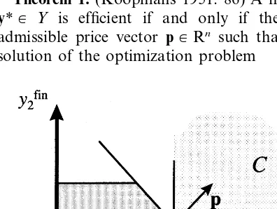
Theorem 1.(Koopmans 1951: 86) A net-output
y* Y is efficient if and only if there is an admissible price vector p Rn such that y* is a
solution of the optimization problem
maxpfinT
yfinsubject to
y Y.
It is enough for an understanding of our ecosys-tem model to explain the main idea of the proof of the implication ‘if the net-outputy*is efficient then there is an admissible price vector...’.10 Let y* be an efficient net-output. The main task is to find an admissible vectorpsuch thaty*is a solution to the optimization problem.
For this purpose, consider the setCof all points
y R which have a properly bigger net-output of final products than y* and also satisfy the factor restrictions (but need not be produced by the given technique):
C={yRn
yfin
−y*fin]0 and y`h}.
The wanted admissible price vectorpis a normal vector of the separating hyperplane between the set of all feasible net-outputsYand the setC(see Fig. 1). The detailed argument is given in the Appendix A.
The theorem allows not only the statement of prices within an economy as was intended by Koopmans, but can also be applied to ecosystems to derive prices there under certain circumstances. It is, of course, a necessary condition for a mean-ingful derivation of ecosystem prices that the as-sumed linear production structure and the restrictions on the primary factors properly de-scribe the transformation processes within the con-sidered ecosystem. The assumptions need to be checked by ecological studies. After this is done it needs to be verified whether the empirically ob-served net-outputy* of the ecosystem is efficient. How this can be done will be shown in Section 3. If y* turns out to be efficient, then prices can be derived.
According to the theorem, the efficiency of the observed net-output is equivalent to the statement ‘the ecosystem realizes the net-output with the highest total value subject to the linear technology and the restrictions of the primary factors’. The total value of net-output is calculated by first weighting the flows of services by pi and then
Fig. 1. Separating hyperplane between the setY of feasible net-outputs and the setCat the efficient pointy*.
10A rather formal proof can be looked up in Koopmans
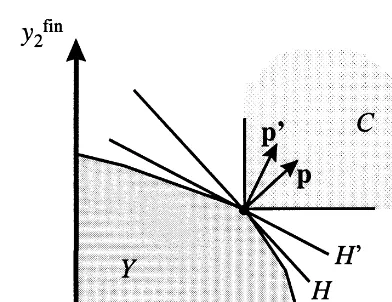
Fig. 2. Situation in which there are several separating hyper-planes and price systems.
this Koopmans takes — at least partly — the First Law of Thermodynamics (the principle of mass and energy conservation) into account. But Koopmans does not explicitly exclude in his model the possi-bility of ‘input without output’. This assumption of ‘free disposal’ also contradicts the mass and energy conservation principle (O’Connor 1993: 268).
One problem that may arise is the ambiguity of the price vector, which we will now investigate. The uniqueness of a price vector (up to a scalar multi-ple) would be a desirable property if we wanted to use the prices for e.g. the aggregation of the varying natural services to a one-dimensional ‘value of total production’. Unfortunately, it may happen that the ecosystem prices derived from our model are not unique. Fig. 2 shows a situation where there are many (even infinitely many) possibilities to place a separating hyperplane betweenYand the setCand, therefore, many different price vectors.
However, we can check for a given situation whether a unique price system exists. If the flows of services between the components of an ecosys-tem are observed, the vertexes and facets of the polyhedron of feasible points can (as we will show in the next section) be calculated. If the observed net-output y* lies not on a vertex or edge of the polyhedron but inside a facet, the price system is unique; in this case the normal vector of the facet (pointing towardsC) is the (up to a scalar) unique price vector (Fig. 1).
3. Calculating ecosystem prices
The applicability of the ecosystem model we developed in Section 2 closely depends on whether prices can be derived from the data observed. We assume that it is possible to observe the net-outputs of the individual activities.13
We will now develop an algorithm to determine the prices. We will first describe the principle of price calculation using a simple example with hypothetical numbers. Then we will explain a general approach for calculating prices and discuss the difficulties that may arise. adding them. These weights of the objective
func-tion can be interpreted as prices of the service flows. If the serviceihas the pricepi, this means that an
additional (marginal) unit of the service i would lead to an increase of the objective function of the magnitudepi. Note that the ecosystem prices are
solely determined by the structure of the transfor-mation processes within the ecosystem and by the restriction of the primary factors.
For economic systems it is widely accepted that the objective function ‘total value of net-output’ (i.e. the national product) is a more or less adequate indicator of social welfare. In order to use our ecosystem prices as surrogates for economic valua-tions of natural goods our interpretation of the weights need to be funded on a similar base: Empirical ecological studies are necessary to check whether our supposition is true that there is a correspondence between the objective function and the ‘well-being’ of the observed ecosystem.11
The existence of a feasible net-output is of course necessary for the derivation of prices. The existence can be shown (using the Theorem) under the assumption which Koopmans (1951: 50) called the ‘impossibility of the Land of Cockaigne’ (Koop-mans 1951: 88). The assumption excludes the unrealistic case of production without inputs.12By
11Note that the price systems of different ecosystems will
probably differ substantially and will not be at once compara-ble.
12The assumption reads formally: There is no level of
productionx`0, such thaty=Ax]0.
13Several ecological studies (see Footnote 3) suggest that
Example. We consider an ecosystem with three activities and three kinds of services. All three activities are populations of plants that produce biomass by means of sunlight and nutrients. In this model biomass is the final product, whereas sunlight and nutrients are the primary inputs. We observe the following net-outputs:
Plant 3
Plant 1 Plant 2 Total
−1
The columns in the center of the table corre-spond to the net-outputs y1,
y2 and
y3 of the activitiesplant1,plant2 andplant 3. The column on the right side is identical with the net-output
y* of the whole ecosystem.y* is given as the sum of y1,y2 and y3.
The first step to calculate prices is to derive the transformation matrix A of the ecosystem from these observations. The coefficients aij of the
ma-trix A are determined from the equation yi j
=
aijxj. If we assume that the level of production
equals 1 for all activities, thenyi j
=aijholds for all
i and j. Hence the observed data can be summa-rized by the following equation:
Ax*=
The matrix A=(aij) describes the
transforma-tion processes that are in principle possible with respect to the assumption of linearity. The set Y={y Rn
y=Ax for an x`0} of all net-out-puts that can be produced by this technology (neglecting the restrictions of the primary factors) forms a convex cone that is spanned by the column vectors a1,…,
am of the matrix
A. The vertex of the cone lies in the origin of the graph. Not all net-outputs that are in principle possi-ble, i.e. which lie within the coneY, are indeed
feasible since the availability of the primary fac-tors is limited. We assume in our example that the observed net-output y* totally uses up both pri-mary factors, sunlight and nutrients. Hence, the factor restrictions can be described by the vector h=(−4,−8, 0)T. The set of feasible outputs Y then consists of those pointsyof the convex cone
Ywhich satisfy the inequation y`h: Y={yRny=Ax for an x`0 and y`
h}.
The next step of the price calculation is to determine the vertexes of the polyhedronY, as we will now explain. The wanted price vector is, as we have shown above, the normal vector of a separating hyperplane between the set
C={yRn
yend
−y*end]
0,y`h}
and the convex polyhedron Y at the observed net-output y*. If the point y* is efficient and lies on the facetFof the polyhedronY, then the facet determines the separating hyperplane (Fig. 1). The normal vector of the facet F is thus the normal vector of a separating hyperplane and, therefore, a price vector of the ecosystem. In order to calcu-late the price vector, the vertexes of the polyhe-dron Y and thus of the facets must first be determined. The facet to which y* belongs must then be examined. The corresponding normal vec-tors represent a respective price system.
In our example the vertices of the polyhedron are characterized by the fact that an activity pro-duces at the highest possible level.14The maximal level of production of activity j solves
max
x
xj subject to Ax]h.
We obtain for the first, second and third activ-ity the maximum levels of production x1= (2, 0, 0)T, x2=(0,8/3, 0)T and x3=(0, 0, 4)T. Thus the vertices e1
,e2 and e3
of the polyhedron Yare
e1
14This characterization is not generally correct. For a
e3
=Ax3
=(−4,−4, 4)T.
The fourth vertex is the origin of the graph 0=
(0, 0, 0)T. The vertex e1
is identical with the observed net-outputy*. Fig. 3 shows the polyhedron Yas well as the pointy*. Note that the four vertexes0,
e1 , e2
and e3
are positioned in a plane, i.e. the 3-dimensional polyhedron is degenerated to a 2-dimensional quadrilateral. To understand this, it must be realized thaty*=e1 can be generated by
activity 1 at production level 2 (i.e. x=(2, 0, 0)T) and also by all three activities at the unit produc-tion level (i.e. x=(1, 1, 1)T). Hence, the activities
a1, a2 and a3, which span the polyhedron Y, are
linearly dependent, i.e. they belong to the same plant.15
All efficient net-outputs lie, as can be seen in Fig. 3, on the junction-line from e1to
e2, because only these net-outputs reach a biomass output of 8 units. Thus we have verified that y*=e1 is efficient. Now we have all the information needed to determine the admissible price vectors. In Fig. 3 it can also be perceived that the vector p=
(0, 0, 1)T is an admissible price vector since the plane Hp defined by p separates at the point y* the polyhedronYfrom the setC.16
The separating (hyper)-planeHp lies parallel to the axis ‘sunlight’
and ‘nutrients’ in the plane of the quadrilateral ABDy*. In our numerical example the price vec-tor is not unique because the efficient net-output
y* observed lies at the vertex e1.17 The plane spanned by the points 0, e1,
e2 and
e3 also sepa-rates YfromC. The corresponding price vectorp%
stands perpendicular to the vectors e1 and e2, i.e.
p% is identical with the solution (0, 1, 1)T of the system of linear equations
y1y2
Á Ã Ã Ã Äp%1
p%2
p%3
 à à à Å
=
−4,−8, 8−8
/3,−8, 8
Á Ã Ã Ã Ä
p%1
p%2
p%3
 à à à Å
=
00
.p% is an admissible price vector, too. The price of the primary nutrients is atp%(in contrast top) not zero.
Fig. 3. Set of feasible net-outputsYand the observed net-out-puty* in the numerical example 1. The 3-dimensional polyhe-dronYis degenerated to a 2-dimensional quadrilateral.
15We have chosen an example with only three services
because it is then possible to graphically display the polyhe-dronY. To avoid another problem (which in general does not occur in models with several final products) we have deter-mined the activities to be linearly dependent. If the numbers of an example with two primary factors and one final product are such that the activities are linearly independent, it can be shown that the observed net-output cannot be efficient and, therefore, no price system can be derived.
16One can easily imagine the location of the setCin Fig. 3:
LetObe the positive orthant of the graph, one gets the setC
by parallel translation ofOby vectory*.
17It is not possible to find an example with three services
All admissible price vectors are represented by the convex combination ofp and p%, i.e. they can be written in the form (0,p, 1)T with 05p51.
The price of the primary factor sunlight is 0, since it is a free factor: A (marginal) reduction of the sunlight used would not lead to a reduction of the produced biomass.
We will now present a general algorithm for the calculation of prices from given data.
1ststep: The net-outputy* of the whole system is calculated from the observed net-outputs of the individual activities.
2nd
step: The restriction of the primary factors h must be determined on the basis of ecological knowledge of the ecosystem. For instance, the restriction of the primary factor ‘rainwater’ may be determined by the amount of rainfall observed. As it may be more difficult to ascertain other restrictions (e.g. the amount of imported nutri-ents), it may be useful to assume that the ob-served net-output y* fully exhausts these restrictions.
3rd step: The vertexes and facets of the polyhe-dron Y must then be calculated and the normal vectors determined for each facet. A method for doing this is described in Klauer (1999: 20 – 22). It is based on mathematical results by Dantzig (1951) which he also uses in his simplex method of linear programming. Now the vectors are admissi-ble according to Definition 3 must be filtered out from the final set of normal vectors {p1,…,
pr}.
4th step: We must check whether the observed net-outputy* is efficient, because only in this case will there be a separating hyperplane between Y and the efficiency coneCat the pointy*. Accord-ing to Theorem 1, y* is efficient if and only if there is an admissible price vector such that y* maxpfin, T
yfin
subject to y Y.
In order to check whether y* is efficient, it is sufficient to check the final set of admissible nor-mal vectors {p1,…,
pr}. Three cases are possible:
1. There is no vector in {p1,…,
pr} such that
y* solves the optimization problem. Then y* is not efficient and no price system can be derived.
2. There is exactly one vector pk in {
p1,…,
pr}
such that y* solves the optimization problem.
Thenpkis the (up to a scalar) unique
admissi-ble price vector.
3. y* solves the optimization problem for the vectors pk1,…,pkl in {p1,…,
pr}. Then all
vec-tors within the convex envelope of pk1,…,pkl
are admissible price systems to y*.
The first case in which y* is not efficient is particularly precarious. This case can be ruled out by an additional assumption: If every activity produces only one final product, which is more-over not produced by any other activity (i.e. it is specific) and if all primary factor restrictions are fully exhausted, theny* is always efficient:18
If the production level of any activity is increased, then (because of the factor restrictions) the production level of some other activity must inevitably be reduced and thus the output of the respective (specific) final product decreases. Nevertheless, whether the ecosystem prices make sense depends on the (ecological) plausibility of this (and the other) assumptions.
4. Discussion: limitations and prospects for the evaluation of natural goods by ecosystem prices
The main result of our model is that prices for the services of an ecosystem can be derived if the net-output observed is efficient. The ecosystem prices are characterized by the fact that the state-ments ‘the observed net-output is efficient’ and ‘the total value of the net-output’ (calculated with these prices) is equivalent. The ecosystem prices are solely determined by the structure of the ecosystem’s transformation processes and by the restriction of the primary factors. If it is empiri-cally verified that the observed net-output is effi-cient (by the method described in Section 3) and if the assumptions of our model prove to be ecolog-ically plausible, the mass of empirical data can be
18The final output ‘plant biomass’ could e.g. be a specific
condensed to aggregated information about the overall state of the ecosystem. This process is comparable to national accounting for economies. Such aggregated information about ecosystems can support decision-making in environmental policy.
Our model has several advantages over the existing approaches to ecosystem prices of Han-non (1985) and Amir (1975, 1987, 1989, 1994, 1995) as described in Section 1. However, our model currently contains a number of restrictions and shortcomings (most of which also occur in Hannon’s and Amir’s models), which ought to be eliminated by further research:
1. As noted before, empirical ecological studies are necessary to check our supposition — that the objective function ‘total value of net-out-put’ corresponds to the well-being of the ob-served ecosystem and — that the assumed linear production structure and the restrictions on the primary factors describe the natural transformation processes sufficiently accu-rately. Once these suppositions are confirmed ecosystem prices reflect the contribution of a net-output to the well-being of the ecosystem. 2. It may happen that the observed net-output of the system is not efficient and no price system can be derived. Under certain assumptions this precarious case can be avoided. However, it is crucial for the application of the model that these additional assumptions prove to be eco-logically plausible, too.
3. It may happen that the derived price system is not unique. If the ecosystem prices are used to assess environmental problems, the different price systems may produce contradictory advice.
4. The model is static. Indeed, the model can be interpreted as quasi-static: If we suppose a myopic objective function which depends only on flows of the actual period and if we assume the ecosystem is in a stationary state, all the results of the model remain valid. But this simple-period structural analysis does not al-low to investigate the structural consequences of changes in the coefficients over time. One consequence of this is that stocks of natural capital cannot be reflected in the model.
How-ever, the build up and exhaustion of natural capital stocks are important for describing natural processes. One starting-point for the dynamization of the model and the consider-ation of stocks in our model could be the study by Malinvaud (1953), which augments the model of Koopmans (1951) with intertem-poral aspects. Furthermore, the studies of Per-rings (1986, 1987) and O’Connor (1993, 1994) take advantage of the duality of quantity and value in a multi-period framework.
5. Another problem of our model is that struc-tural changes to the ecosystem, i.e. the occur-rence and disappearance of components such as the migration of new species or the local extinction of others, cannot be reflected. If the structure of the ecosystem changes, the respec-tive price systems cannot be compared. The probability of a structure becoming apparent in the model decreases with the level of aggre-gation of the components. However, a high level of aggregation means that energy and material flows can only be coarsely compre-hended by the model and the information contained in the ecosystem prices is compara-tively low.
Since neoclassical methods of evaluating natu-ral goods also face severe practical difficulties as well as theoretical weaknesses, we want to discuss the following questions:
1. To what extent are our ecosystem prices suit-able for evaluating natural goods?
Values that are derived independently of human beings, e.g. those which were already in the world before humans occurred, are called ecocentric val-ues (Krebs, 1997). Are the prices we have derived in our ecosystem model ecocentric prices? Does the use of ecosystem prices to evaluate natural goods mark a shift away from anthropocentrism towards ecocentrism? In our opinion this is not the case. Using ecosystem prices means that infor-mation on the relationships in nature flows into the decision process. However, the resulting eval-uations or decisions need not necessarily be adopted by society, which can always reject these evaluations.
The German Academy of Science doubts that a departure from anthropocentrism is at all possible when evaluating nature (1992: 27, our transla-tion): ‘Since Man has to prevail and liberate himself vis-a`-vis his environment, he is unable to position himself as an apparently neutral observer and judge over the environments of all living beings, granting each living being with a patroniz-ing attitude the same right to life.’ It is therefore justified to speak of an ‘absence of a way out of anthropocentrism’ when dealing with the evalua-tion of nature (Academy of Science, 1992: 32; Hofmann, 1988: 277).
Nevertheless, there is no direct relation between ecosystem prices and evaluations by the individu-als of society. This means that ecosystem prices cannot be directly compared to economic prices. Moreover, recommendations cannot be directly concluded for actions for society from ecosystem prices since they reflect the functional interrela-tions in an ecosystem but not directly the social desirability. However, the aggregate information about functional interrelations can of course sup-port the decision-making process.
The prices that can be derived from these ap-proaches can be used as surrogates for economic prices. This should in particular be taken into consideration if for natural goods no market ex-ists and the respective neoclassical methods of evaluation (contingent evaluation method, hedo-nic pricing, travel cost method) are too expensive or the results are unsatisfactory (Hausman, 1993; Hanley and Spash, 1993).
To sum up, we believe that the derivation of prices in ecosystems is a promising aid to deci-sion-making if traditional economic evaluation methods cannot be successfully applied. However, more research is needed before ecosystem prices can be put to practical use. In particular, ecosys-tem studies should be undertaken in order to empirically confirm that the model (and in partic-ular the objective function) positively describes the behavior of the system and that the prices positively reflect the functioning of the ecosystem.
Acknowledgements
The author gratefully acknowledges critical and helpful comments by Shmuel Amir, Malte Faber, Manuel Frondel, Bruce Hannon and Frank Jo¨st as well as two anonymous referees on earlier drafts of this paper.
Appendix A
In this appendix the proof of the implication ‘if the net-output y* is efficient then there is an admissible price vector...’ of Theorem 1 is scratched.
Let y* be an efficient net-output. The set C={yRn
yfin
−y*fin]0 and y`h}
is not closed (note the definition of ], footnote 8) and y*Q C since it does not holdy*fin]y*fin. The closureCof the setCis a convex cone whose vertex is the pointy*. The edges of the coneClie parallel to the axis of the graph in the positive direction (Fig. 1). The set C as well as the set of feasible net-outputs Y are convex. Since y* is efficient, CandYare disjunct. Therefore, there is a separating hyperplane H between C and Y (Hadley 1961: 6 – 6). This hyperplane is uniquely determined (up to multiplication by a positive scalar) by a normal vector p at the net-outputy* pointing at C:
H={y RnpT
y=pT
y*} (Fig. 1).
Let us assume for the moment thatpis admissi-ble according to Definition 3. All y Y are con-tained in the halfspace HY={yR
n
pT(
y−y*)
0}. Sincep\
pri=0 and by definition
y* =
is non negative, such that
0`pfinT(yfin−y*fin)
for allyY. Therefore, y* is indeed a solution of the optimization problem.
It remains to show that the separating hyper-plane can be chosen such that the normal vectorp
is admissible. This part of the proof which is only of minor importance for an understanding of the ecosystem prices can be found in (Klauer 1998: 171 – 172).
References
Academy of Science (Akademie der Wissenschaften zu Berlin, Arbeitsgruppe Umweltstandards), 1992. Umwelt-standards: Grundlagen, Tatsachen und Bewertungen am Beispiel des Strahlenrisikos. Walter de Gruyter, Berlin, New York.
Amir, S., 1975. Equilibrium in Ecological Systems. PhD the-sis. (in Hebrew, with English summary). Hebrew Univer-sity of Jerusalem, Jerusalem.
Amir, S., 1987. Energy pricing, biomass accumulation and project appraisal: a thermodynamic approach to the eco-nomics of ecosystem management. In: Pillet, G., Murota, T. (Eds.), Environmental Economics: The Analysis of a Major Interface. Roland Leimgruber, Genf, pp. 53 – 108. Amir, S., 1989. On the use of ecological prices and system
— wide indicators derived therefrom to quantify man’s impact on the ecosystem. Ecol. Econ. 1, 203 – 231. Amir, S., 1994. The role of thermodynamics in the study of
economic and ecological systems. Ecol. Econ. 10, 125 – 142.
Amir, S., 1995. Welfare maximization in economic theory: another viewpoint. Struct. Chang. Econ. Dyn. 6, 359 – 376.
Arrow, K.J., Debreu, G., 1954. Existence of equilibrium for a competitive economy. Econometrica 22, 265 – 290.
Arrow, K.J., Hahn, F.H., 1971. General Competitive Analy-sis. Holden – Day, San Francisco. Oliver and Boyd, Edin-burgh.
Dame, R., Patten, B.C., 1981. Analysis of energy flows in an intertidal oyster reef. Mar. Ecol. — Prog. Ser. 5, 115 – 124.
Dantzig, G.B., 1951. Maximization of a linear function of variables subject to linear inequalities. In: Koopmans, T.C. (Ed.), Activity Analysis of Production and Alloca-tion. Wiley, NY, pp. 339 – 347.
Debreu, G., 1959. Theory of Value. Wiley, New York. Fasham, M.J.R., 1985. Flow analysis of materials in the
marine euphotic zone. In: Ulanowicz, R.E., und Platt, T. (Eds.), Ecosystem Theory for Biological Oceanography Canadian Bulletin of Fisheries and Aquatic Science, pp. 139 – 175.
Hadley, G., 1961. Linear Algebra. Addison – Wesley, Read-ing, MA.
Hanley, N., Spash, C., 1993. Cost-Benefit Analysis and the Environment. Edward Elgar, Aldershot.
Hannon, B., 1976. Marginal product pricing in the ecosys-tem. J. Theor. Biol. 56, 253 – 267.
Hannon, B., 1985. Linear dynamic ecosystems. J. Theor. Biol. 116, 89 – 110.
Hannon, B., 1995. Input – output economics and ecology. Struct. Chang. Econ. Dyn. 6, 331 – 333.
Hannon, B., Costanza, R., Herendeen, R.A., 1986. Measures of energy cost and values in ecosystems. J. Environ. Econ. Manag. 13, 391 – 401.
Hausman, J.A. (Ed.), 1993. Contingent Valuation: A Critical Assessment. North-Holland, Amsterdam.
Hofmann, H., 1988. Natur und Naturschutz im Spiegel des Verfassungsrechts. Juristenzeitung 43, 265 – 278.
Klauer, B., 1998. Nachhaltigkeit und Naturbewertung: Welchen Beitrag kann das o¨konomische Konzept der Preise zur Operationalisierung von Nachhaltigkeit leisten? Pysika, Heidelberg.
Klauer, B., 1999. Pricing in Ecosystems: A Generalized Lin-ear Production Model. UFZ-Discussion Papers 2/1999. UFZ Centre for Environmental Research Leipzig-Halle, Leipzig.
Koopmans, T.C., 1951. The analysis of production as an efficient combination of activities. In: Koopmans, T.C. (Ed.), Activity Analysis of Production and Allocation. Wiley, New York, pp. 147 – 154.
Krebs, A., 1997. Ethics of Nature. A Map, Amsterdam, Atlanta.
Malinvaud, E., 1953. Capital accumulation and efficient allo-cation of resources. Econometrica 21, 233 – 269.
Perrings, C., 1986. Conservation of mass and instability in a dynamic economy-environment system. J. Environ. Econ. Manag. 13, 199 – 211.
O’Connor, M., 1993. Entropic irreversibility and uncon-trolled technological change in economy and environ-ment. J. Evol. Econ. 3, 285 – 315.
O’Connor, M., 1994. Entropy liberty and catastrophe: on the physics and metaphysics of waste perspectives on economic analysis. In: Burley, P., Foster, J. (Eds.), nomics and Thermodynamics: New Perspectives on Eco-nomic Analysis. Kluwer, Dordrecht, pp. 119 – 181. Odum, E.P., 1969. The strategy of ecosystem development.
Science 164, 262 – 270.
Odum, H.T., 1957. Trophic structure and productivity of Silver Springs, Florida. Ecological. Monographs. 27, 55 – 112.
Reichle, D.E., O’Neill, R.V., Harris, W.F., 1975. Prin-ciples of energy and material exchange in ecosystems. In: Dobben, W.H, Lowe-McConell, R.H. (Eds.),
Unify-ing Concepts in Ecology. W. Jung, Den Haag, pp. 27 – 43.
Samuelson, P.A., 1951. Abstract of a theorem concerning substitutability in open Leontief models. In: Koopmans, T.C. (Ed.), Activity Analysis of Production and Alloca-tion. Wiley, New York, pp. 142 – 146.
Samuelson, P.A., 1964. Economics: An Introductory Analysis. 6th ed. McGraw – Hill, New York.
Steel, J.H., 1974. The Structure of Marine Ecosystems. Harvard University Press, Cambridge, MA.
Tilly, L.J., 1968. The structure and dynamics of Cone Spring. Ecol. Monogr. 38, 169 – 197.
von Neumann, J., 1945. A model of general economic equi-librium. Rev. Econ. Stud. 13, 1 – 9.
Whittaker, R.H., 1975. Communities and Ecosystems. Macmil-lan, New York.