Variations on a
k
–
ε
turbulence model for supersonic boundary layer computations
D. Guézengara,b, J. Francescattoa, H. Guillarda,*, J.-P. Dussaugeb
aINRIA, Projet SINUS, B.P. 93, 2004 Route des Lucioles, 06902 Sophia Antipolis cedex, France bIRPHE, U.M. CNRS-Universités No. 6594, 12 Avenue Général Leclerc, 13003 Marseille, France
(Received 15 January 1998; revised 6 October 1998; accepted 22 October 1998)
Abstract – Several modifications of the baselinek–εmodel are considered for the computation of supersonic boundary layers on an adiabatic flat plate, up to Mach number 5. The numerical computations are performed with particular reference to well documented experiments. Three versions of a two-equation low-Reynolds number model and a two-layer model are used. They were originally defined for incompressible flows and have to be extended to compressible cases. Slight alterations of the original formulation are necessary to obtain good numerical performances. The use of compressibility models is also investigated, as well as a possible simple modification of the dissipation rate equation to take into account the turbulence balance in the logarithmic region. The numerical results are in good agreement with the experimental data. Some numerical issues are addressed and the importance of suitable boundary conditions is pointed out.Elsevier, Paris
Nomenclature
wsubscript Wall value a Local speed of sound
esubscript External value V =R0U√ρ/ρwdU van Driest transformation
x Horizontal coordinate τ Shear stress tensor
y Vertical coordinate uτ =
√
τw/ρw Friction velocity
ρ Fluid density µ Dynamic molecular viscosity
u Horizontal velocity ν=µ/ρ Kinematic molecular viscosity
v Vertical velocity µt Dynamic eddy viscosity
p Static pressure y+=uτy/νw Non-dimensional wall distance T Static temperature cf =2τw/(ρeu2e) Skin friction coefficient
k Kinetic energy of turbulence P Turbulence production term
ε Solenoidal dissipation rate Cp Specific heat at constant pressure
M Mach number P rt =0.9 Turbulent Prandtl number
Tt Total temperature Q= −(µtCp/P rt)(∂T /∂y) Heat flux εc Compressible dissipation rate Mt =
√
2k/a Turbulent Mach number
εt =ε+εc Total dissipation rate
1. Introduction
One of the leading effect of compressibility in supersonic boundary layers is the occurrence of large density gradients across the layer. As a result, mean velocity scaling differs from its subsonic equivalent and the correct inner similarity law is the van Driest compressible law of the wall (van Driest [1]):
V
whereV is the van Driest transformed velocity:
V =
Although the constants in (1) can in principle be functions of the friction Mach number (Bradshaw [2]), the extensive review by Fernholz and Finley [3] shows that most of the available experimental data follow (1) with
κ=0.41 and C∗∼5.2. Expression (1) can therefore be considered as the present consensus that turbulence models should reproduce.
Another effect of supersonic flow is the presence of additional terms in the turbulent kinetic energy budget. These terms are either explicitly present in the exact averaged equations (pressure dilatation correlation
p′(∂ui′′/∂xi)) or implicitly included in the definition of the turbulent kinetic energy rate of dissipation
(dilatation dissipation). In principle, an appropriate compressible modelling should not ignore these terms. Despite these well-known facts, compressible shear flows are usually computed with little or no modification of the models originally developed for incompressible flows. A standard attitude might be just to move to the Favre mass-weighted averages and hope for the best. However, several recent works have questioned the validity of such an approach for supersonic boundary layers: Huang et al. [4] shows that the standard k–ε
model is inconsistent with the van Driest law (1) and that the coefficients in turbulence models must be a function of density gradients. They proposed models to reduce this density gradient effect to an insignificant level. Following the analysis of Huang et al. [4], Aupoix and Viala [5] have experimented with the inclusion of density gradient terms in the dissipation equation.
Due to their success for compressible mixing layer predictions, the use of the so-called compressibility models to evaluate the pressure–dilatation correlations or the dilatation dissipation have also received a lot of attention (Aupoix and Viala [5], Huang et al. [4], Mohammadi and Pironneau [6]) for boundary layer computations.
Our goal in this paper is to review the use of different variants of thek–ε model for supersonic boundary layers up to Mach 5. Aside from the basic k–ε model with wall functions, we have studied the use of three different low-Reynolds models and a two-layer model inspired by the work of Chen and Patel [7]. We will also report on the use of compressibility models and test an original model allowing the Prandtl number (σε)
introduced to model the diffusion of dissipation rate, to be dependent on density variations in a way originally suggested by Huang et al. [4]. The test-cases on which these studies have been conducted are the Mach 1.76 experiment of Dussauge et al. (Fernholz and Finley [8]) and the Mach 4.52 experiment of Mabey et al. (Fernholz and Finley [9]).
of models and of numerics are. We believe that such effects are more important in compressible flows than in incompressible ones. Therefore to make fair comparisons, for each physical modelling (near-wall, compressibility and density variation effects), test-cases were performed with the same numerical method, in order to solve the averaged Navier–Stokes equations coupled to thek–ε model. In this paper, we also give some examples of the influence of the numerical conditions on the results and emphasize the role that proper boundary conditions can have.
2. Description of the two-equation models
The governing equations are obtained by Reynolds averaging the compressible Navier–Stokes equations, and modelling the Reynolds stresses by the Boussinesq assumption. The closure of the system is realized by the well-knownk–εturbulence model which can be written as
∂ρk
where the right-hand sides of (3), (4) contain the production and the dissipation terms forρkandρε:
Sk= −ρε+P and Sε=cε1fε1
1.3, 1.44, 1.92 for the standardk–ε model. The values used in the low-Reynolds number models are given in the Appendix.fε1,fε2,fµare correction functions whose role is to enforce a correct behaviour of the turbulent
variables close to the wall. They will be defined below.
2.1. Near-wall modelling for compressible flows
2.1.1. The wall-function approach
The wall-function technique avoids the modelling problem near the wall by imposing boundary conditions at a small distance δ from the solid wall, where local equilibrium is achieved. These boundary conditions are deduced from the similarity solutions of the boundary layer equations which takes the following form for compressible flows with zero pressure gradient:
horizontal momentum equation: τ =τw, (5a)
energy equation: Q−uτ=Qw, (5b)
whereτ = −ρug′′v′′+µ(∂u/∂y)is the shear stress,Q=ρCpu]′′T′′−λ(∂T /∂y)the heat flux, and subscript w
denotes the values at the wall. Expressing (5a) with Prandtl’s mixing length model yields
where the friction velocityuτ is defined byuτ=
where V is the van Driest [1] transformed velocity defined by relation (2). An explicit expression for the van Driest transformed velocityV can be obtained by assuming that the pressure is constant at each station (ρw/ρ=T /Tw) and by using a gradient expression for the heat flux:
Q= −µtCp
P rt ∂T ∂y
with a constant turbulent Prandtl numberP rt in the layer. This gives from (5b)
T
and expression (6) can be integrated to give (van Driest [1], Fernholz and Finley [3], Huang et al. [4])
V =√B
This expression will be used to give the boundary conditions needed for the tangential velocity at a distanceδ
from the solid wall. For adiabatic flows(Qw=0), we deduce from (5b) an homogeneous Neumann boundary
condition for the energy equation. Finally, to specify the boundary conditions on the turbulent variables at
y=δ, the relation−ug′′v′′=pCµkis used together with the local equilibrium assumption between production
and dissipation:
The standardk–ε model is not valid in regions close to the wall where the viscous effects are important. In low-Reynolds number modelling, the molecular effects and the proximity of the wall are taken into account by the introduction of damping functionsfε1,fε2 andfµthat enforce a proper behavior of the turbulent quantities.
In this study, we have compared three low-Reynolds number models namely, the model of Lam–Bremhorst (Lam and Bremhorst [10]) and the more recent improved models of Nagano–Tagawa (Nagano and Tagawa [11]) and Speziale–Abid–Anderson (Speziale et al. [12]). The precise definition of these models is recalled in the Appendix. The three models were originally defined for incompressible flows with the assumption that the low-Reynolds number effect can be represented by a local “turbulence” Reynolds number, respectively:
As a consequence of Morkovin’s hypothesis, it will be assumed that such corrections do not depend on Mach number, and only a Reynolds number dependence will be retained. Now, in supersonic flows, density and viscosity are not constant, so that the definition of the turbulent Reynolds number has to be reconsidered. For example, in the previous expressions, we can choose, for the kinematic viscosity, either the wall valueνw or a
local valueν(y). In the present work, the classical definition ofy+=yuτ/νwwith the viscosity taken at the wall
has been retained.y+ is as usual the ratio of the distance to the viscous length scale at the wall. Experiments have shown that such a parameter provides a good representation, presumably universal, of the velocity profile in the wall region. To define Ry and Rt, we have now to define a turbulent velocity scale. It is recalled (see
for example Smith and Dussauge [13]) that in the constant shear zone, the scale for velocity fluctuations is
√
ρ/ρw
√
k instead of √k; combining this with the logarithmic law for the van Driest transformed velocity suggests the following expressions forRyandRt:
Rt =
and in practice,RyandRthave been computed from the latter relationships. Note that definitions (8) imply that Ry=C−µ1/4y+and Rt =κy+/Cµ. Such are the choices made in the present study. Other choices are possible
(see for instance Aupoix and Viala [14] for a comparison of different definitions ofy+).
To close the description of the low-Reynolds number model, we need to specify the boundary conditions used at y =0. On an adiabatic wall, no-slip conditions and zero heat flux are used for the momentum and energy equations while an homogeneous Dirichlet boundary condition is used for the turbulent kinetic energy. A problem comes from the specification of the turbulent dissipation rate at the wall. The type of boundary condition which is used for this variable has a tremendous influence on the stability of the numerical computations. We found that the boundary condition suggested in Chapman and Kuhn [15]:
ε|y=0=
where the value ofδ corresponds to the first mesh increment in theydirection, leads to the best results in term of accuracy and robustness of the numerical algorithm.
2.1.3. A two-layer model
Two-equation models, with low-Reynolds number modelling, are not very robust and it is often difficult to obtain convergence to a steady state. Moreover, they require over refined meshes to describe conveniently the large variations of the turbulent quantities close to the wall. Therefore, we have also tested a two-layer model, inspired by the work in Chen and Patel [7]. For such an approach, in regions whereRy>200 the standardk–ε
model is used. However, in regions contiguous to the solid-wall surface, whereRy<200, the one-equation
low-Reynolds number model of Wolfshstein [16] is used. This model solves the mean-flow equations and a modelled equation for the turbulent kinetic energy, whilst the characteristic length scales are determined via algebraic relations. In the original (low-speed) formulation of the model, the eddy viscosity and the dissipation rate of turbulent kinetic energy are defined by
and length scaleslµandlε are
lµ=κCµ−3/4yfµ and lε=κCµ−3/4yfε, (10)
wherefµandfεare two correction functions:
fµ=1−exp
−R
y Aµ
, Aµ=70, fε=1−exp
−R
y
2κ Cµ−3/4
.
Such functions have the form of a van Driest damping and are introduced to mimic the correct behavior when the wall is approached and when the flow is dominated by viscous effects. This influence may depend on density variations. In Viala [17], several adaptations have been proposed. In the present work, it has been found that the following modification:
lµ=κCµ−3/4
s
ρw ρ yfµ
has a very positive influence on the accuracy of the results.
In the numerical implementation, we have found it useful to introduce a “buffer” zone between the regions where the two models are used. Specifically, for 180< Ry<220, the eddy viscosity is assumed to vary linearly
between the values given by the two models:
µt=αµ two-layer
t +(1−α)µkt−ε, α=
220−Ry
40 .
Such a procedure ensures that the eddy viscosity will vary smoothly between the limiting values given by the two models. However, the extension of this procedure to more complex flows or geometries may raise some problems.
Finally, the dissipation rate equation uses Dirichlet boundary conditions forRy<200, with the values given
by the one-equation model.
2.2. High-speed flow modelling
In high-speed turbulent flow modelling, two contributions can be distinguished: a high Mach number effect and a density variation effect. Although these two contributions are not independent, they are usually modelled separately. In this section, the models which are used in this study are described.
2.3. Compressibility effects
incompressible expressionε=ν(∂uj′/∂xi)(∂uj′/∂xi). It was assumed (Sarkar et al. [18], Sarkar et al. [20],
Zeman [19], Wilcox [21]) that the dissipation can be split into a solenoidal and a compressible part:
εt =ε+εc.
εrepresents the incompressible dissipation which is described by the standardε-equation. The second effect of compressibility was represented by the pressure-divergence terms. It was proposed to model these two effects as a function of the turbulent Mach number Mt =
√
2k/(3γ RT ). These models were applied successfully to the case of mixing layers, but seemed less appropriate for the computation of boundary layers. Further work in numerical simulation was performed for supersonic homogeneous shear flows (Sarkar [22]), channel flows (Huang et al. [23]) and annular mixing layers (Freund et al. [24]). Sarkar’s work [22] underlined the importance of the “gradient Mach number” similar to the concept introduced in distortion analysis by Durbin and Zeman [25] and by Jacquin et al. [26]:
Mg=
l(∂U/∂y) a ,
wherelis some integral scale of turbulence. Depending on the value ofMg, the role of pressure is modified
and therefore the anisotropy of turbulent stresses may be altered. Moreover, Sarkar [22] and Simone et al. [27] suggested that dissipation is not crucially altered, even in severe conditions of compressibility and that pressure divergence terms can be often neglected. Recent work by Ristorcelli [28], Ristorcelli and Blaisdell [29], Fauchet et al. [30] and Fauchet [31] have also brought some insights into this question.
A conclusion of these recent works is that for small turbulent Mach numbers, the dilatation dissipation varies likeMt4. Small perturbation analysis of the compressible flow equations has led Ristorcelli [28] to propose that
for turbulent flows out of equilibrium, pressure-divergence terms are proportional toMt2, but can probably be neglected in equilibrium flows in which production balances dissipation.
Another conclusion is that the consequence of the changes in the structure of the pressure field is probably the alteration of the anisotropy of turbulence, an effect strong enough to explain the inhibition of turbulent transport in supersonic mixing layers. Similar properties have been found in the simulation of an annular mixing layer by Freund et al. [24]. It should be noted however that there exist no systematic experiments to check these conclusions. In the supersonic channel flow computed by Huang et al. [23], it is clear that in wall flows, even at a nominal Mach number of 5, the level of compressible dissipation and of pressure-divergence terms is smaller than in mixing layers.
What has been done in the present work is to use some of the compressible turbulence models and to check their behaviour in our computations. They were used with the classical interpretation of modification of the dissipation rate. As a matter of fact, in some cases, the models proposed for the dilatation dissipation can also be considered as a measure of the global effect of compressibility on production. For example, consider the simple case when production balances dissipation:
−ug′′v′′∂U
∂y =ε+εc,
and express the dilatation dissipation in the formεc=εf (Mt). The previous equality can be rewritten as
−ug′′v′′∂U
If εc is not large compared to ε, ε/P is close to 1, and the dilatation dissipation appears as a rough but
situations,Mg andMt are linked to each other in a rather straightforward way. Therefore, some of the existing
models have been tested in the present computations. We have used various expressions forεc from different
authors. They all expressεc as a function of the turbulent Mach numberMt2=2k/(γ RT ),εc=f (Mt)ε. The
whereH is the Heaviside step function. In the following, we will note these models respectively by SEHK, ZEMAN and WILCOX.
A second important effect present in these models is represented by the pressure-divergence terms:p′∇.u′′. This term is modelled in the present study as in Sarkar et al. [20], Sarkar [22] by a function of the production term and of the solenoidal dissipation (referenced by SARKAR in the sequel):
p′∇.u′′= −0.15×P.Mt+0.2×ρε.M2
t.
This last model will be used with the SEHK model for the compressible dissipation.
Such models have been developed for second-order turbulence closures in which the Reynolds stresses are obtained from transport equations. In thek–εmodel, the Reynolds stresses are expressed with the eddy viscosity
µt =Cµρk2/ε and the question of the value of ε which must be used in this expression can be discussed.
An extensive study of the mixing layer configuration (Guézengar and Guillard [32]) shows that the choice
µt=Cµρk2/(ε+εc), except in the solenoidal dissipation transport equation whereµt =Cµρk2/ε, gives the
better results.
2.3.1. Density gradient effects
According to Huang et al. [4], the standard k–ε model cannot satisfy the turbulent energy balance in the logarithmic region of a boundary layer, when significant density gradients exist. Their analysis starts from the boundary layer equations for thekandεvariables in the equilibrium zone:
Introducing expressions (7), considered at the locationy instead ofδin the above equations and assuming that
σε is constant in a section leads to the following relation between the modelling constants appearing in the ε-equation:
model. For incompressible flows, we recover the standard expression:
σε(Cε2−Cε1) κ2
q
but in high speed flows, there is no reasons for the second term of the right-hand side of (13) to be zero. This inconsistency yields an overestimation of the slope of the logarithmic region and conversely an underestimation of the skin friction coefficient.
Huang et al.’s [4] work is the first which points out that the k–ε model, with constant coefficients, cannot reproduce the logarithmic law, when significant density gradients exist. They proposed two different approaches: firstly a variation ofCε1with density, and secondly a new sort of model (likek–ε5/6) to minimize
theai coefficients, and so, by the way, the density influence. Optimization of theCε1constant leads to values
far from the current ones and finally the authors favor the use of other models which reduce the density effect to a lower level, but they are not totally satisfactory.
Aupoix and Viala [14] accepted Huang et al.’s analysis but used another solution. They proposed to improve theε-equation to make it consistent with the turbulence balance. They introduced the second term of the right-hand side of (13) in the dissipation equation to force the logarithmic balance, and they interpret the additional terms as a “modified” diffusion term. The result of this modification is to cancel the density gradients in (13) and to allow the use of a constantσεparameter while preserving the compatibility with the logarithmic law.
Here we try a different strategy and instead look for a relation between σε and the density to make the ε-equation compatible with the compressible law of the wall. Our goal is to insure the turbulence balance by taking into account density gradient effects through a variableσε coefficient. Introducing expressions (7) in
Eqs (12) yields a first-order ordinary differential equation forσε. It has been checked in shear flow computations
(Guézengar [33]) that the coefficient of the derivative ofσεin this ordinary differential equation is small, out of
the viscous zone. Moreover the terms involving the second derivative of the density are also small. Therefore, with a good accuracy, we can consider relation (13) witha2=0 as defining the local value of the modelling
coefficientσε:
Forκ =0.41 and in the absence of density gradients, this relation gives σε≃1.17. The standard value used
in incompressible flows isσε=1.3. Therefore, to allow a consistent comparison between the performances of
the standard model and those of the model using the density gradient correction (14) we will use the following expression:
For the numerical resolution of the full Navier–Stokes equations, the spatial approximation used in this study is a combination of finite-volume and finite-element methods.
Assuming that the computational domainis polygonal, we consider a triangulationτh ofand associate
with this triangulation a dual finite-volume partition ofmade of the control volumesCibuilt from the triangle
Figure 1. Median cellCi. equations in the compact form
∂W
∂t + ∇.F (W )= ∇.P (W )+S(W ),
whereW =(ρ , ρu, ρv, ρe, ρk, ρε)t is the vector of the unknowns,F are the hyperbolic terms,P represent the
diffusive ones andSis the source term. The spatial approximation is done using a finite-volume method on the dual control volume mesh to compute the hyperbolic terms while the remaining terms are integrated by a finite-element method on the triangulationτh. A Roe approximate Riemann solver is used for the approximation of the
hyperbolic terms of mean variable(ρ , ρu, ρv, ρe)t equations while the positivity-preserving multi-component Riemann flux proposed in Larrouturou [34] is considered for the approximation of the convective terms of theρk and ρε equations. A second-order MUSCL type scheme is used to increase the spatial accuracy. In the results presented here, we do not use any limiters on the mean variables but we do use limiters on the turbulent ones. Actually, in the boundary layer computations that we report here, the numerical Reynolds number||Eu||h/νt is moderate and limiters are not necessary. Therefore, the spatial approximation of the mean
variables is guaranteed to be second-order accurate. More details on this spatial approximation can be found in Fezoui et al. [35], Dervieux [36], Olivier and Larrouturou [37], and Guillard [38].
Discrete equations are then marched forward in time using an implicit first-order preconditioning and a local time stepping. The steady state is considered as being reached when a normalized residual of 10−6 based on
the turbulent kinetic energy equation is attained.
3.2. The problem of the inlet boundary conditions
Since a boundary layer is parabolic in the streamwise direction, the flow is highly dependent on the prescribed inlet boundary conditions. Unfortunately, the experimental data are not complete enough to prescribe all the variables which are needed for the computations. We discuss here the way we have re-constructed the inlet boundary profiles.
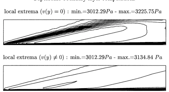
Figure 2.Me=4.52: Isovalues of pressure (v(y)=0 andv(y)6=0 for inlet profile). The interval between the isovalues is1p=15.33 Pa. The first
isovalue corresponds toP=3025.33 Pa.
results. Therefore, for high speed flows, we found it necessary to prescribe a non-zero vertical velocity profile in the inlet section. The strategy we used to construct the profile is the following: Firstly, we have performed a numerical simulation with a zero vertical velocity as inlet boundary condition. Then, the vertical velocity profile, in the last section of the computational domain, is made non-dimensional assuming that the flow is self-similar and this new profile is used as boundary condition for a second computation. This process can be repeated until no noticeable differences can be seen in the results. However, in practice we found that the changes in the results were minor after a second computation. Figure 2 illustrates the success of this strategy: it can be seen that the large pressure wave which resulted from a zero vertical velocity boundary condition has almost disappeared after a second computation and the pressure variation in the outerflow is at worst 1.5% of the inflow pressure.
The other mean variables (horizontal velocity and temperature) are available from the experimental data and are used as inlet conditions in thek–ε computations with wall functions. However, the experimental data do not extend sufficiently close to the wall for the low-Reynolds number models. To extend them to the wall vicinity, we fit a fifth-order polynomial iny+between y+=0 and the first data point. The six coefficients of this polynomial were computed using the continuity of the velocity and of its first and second derivatives at the first data point; this gives three relations between the coefficients. The remaining three conditions were obtained byu=∂2u/∂y2=0 andµ(∂u/∂y)=τwaty=0. Figure 3 shows the inlet horizontal velocity profile obtained
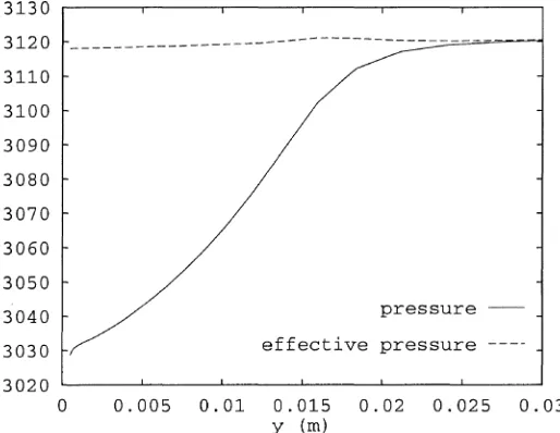
with this method. It was found that this procedure ensures a good compatibility between experimental data and low-Reynolds number models, while other ways to define inlet boundary conditions on mean variables that we tested have lead to convergence problems. The same strategy was used for the temperature using a fourth-order polynomial imposing the continuity of the temperature and of its first derivative at the first experimental data point together with the specification of the wall temperature and of the condition∂T /∂y=0 aty=0. We also mention that instead of a constant pressure across the layer, we impose, as inlet condition, that the effective pressure:p+2/(3ρk)is constant across the layer. This correction reaches 3% in the experiment of Mabey. This can be seen from figure 4 which displays the pressure and the effective pressure at the station x=1.384 m. Although small, this correction has a noticeable influence on the accuracy of the results and we have found that it improves the skin friction prediction slightly. Finally, the inlet turbulent variable profiles were not available from the experimental data. Therefore, we had to specify them by other means. For the Mabey Me=4.52
test-case, they have been computed using the eddy-BL code of Wilcox [39] which solves the boundary layer equations. For the Dussauge Me=1.76 experiment, the profiles were generated assuming a mixing length
Figure 3.Me=4.52: Inlet boundary profile of the horizontal velocity.
Figure 4.Me=4.52: Pressure and effective pressure profile atx=1.384 m.
Since the goal of this study is to provide a detailed comparison between the results of the tested models and specific experiments, a practical important question is to ensure compatibility between the inlet boundary conditions and the internal dynamics of models. In general, a lack of compatibility between the modelled equations and the boundary conditions generates spurious oscillations near the boundary. These oscillations can very often be seen in turbulent computations. An example is given in figure 7 for the MabeyMe=4.52
experiment using different turbulence models.
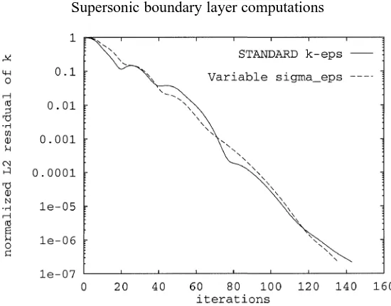
Figure 5.Me=4.52: Comparison of the convergence rates of the standardk–εmodel and of the variableσεmodel (with wall functions).
larger set of inflow quantities, not available from the experiments, have to be prescribed. We notice for instance, with the low-Reynolds number models, an initial steep fall of the skin friction coefficient near the boundary (figure 14). This initial decrease is of limited extent and the computations very soon recover a correct value for Cf. We mention that this effect is more important with the two-equation low-Reynolds number models
while the two-layer model appears to be less sensitive to this initial effect of the boundary conditions.
3.3. Convergence to steady state
An important point in the practical evaluation of a model is its capability rapidly to reach a steady state. For all the models tested here, with the important exception of the two-equation low-Reynolds number models, we do not experience any convergence problem and the convergence rate of the basick–ε model with law of the wall is preserved by the modified models.
For instance, figure 5 compares, with thek–εmodel using wall functions, the convergence rates obtained for the standard model (σε=1.3) and for model (15) involving a density gradient dependence of the coefficientσε.
The corresponding computations were made for boundary layer at Mach number 4.52 on a 41×41 mesh and the convergence rates displayed in figure 5 are representative of what was obtained with other models. This kind of computation typically requires 5 min of CPU time on a Dec Alpha 600/266 MHz workstation. The case of the low-Reynolds number models is very different. In addition of requiring a very fine mesh to yield accurate results, they appear to be numerically fragile and their convergence to steady state is excessively low. Typically, on a 113×81 mesh, they require more than 4000 iterations to reach a steady state. A closer examination shows that the parameter Rt is mainly responsible of such a behavior. It appears that in the early stages of
the convergence, the near wall dissipation rate experiences large fluctuations. As a consequence, the parameter
Rt=√ρ/ρwk2/(νwε)may become ill-defined. This considerably slows down convergence. Therefore, in order
to improve the convergence of the iterative method, the near wall treatment was modified by setting for the three low-Reynolds number models:
Rt =Ry lµ
y fory
Figure 6.Me=4.52: Convergence history with implicit algorithms for different models.
wherelµis the algebraic length scale defined in (10). In figure 6, it is seen that such a modification improves
the numerical behavior of low-Reynolds number models in a decisive manner. In the caption, “standard model” holds for any of the low-Reynolds number models combined with the original definition ofRt, other models
use modification (16) and have a much faster convergence. It appears that on the same mesh, low-Reynolds number models now converge to steady state with approximately the same rate than the two-layer model.
4. Numerical results
4.1. Validation test-cases
The validation test-cases presented consist of the development of turbulent boundary layers on an adiabatic flat plate with zero pressure gradient, for two Mach numbers. The first one is a boundary layer in which the effects of compressibility are weak, the experiment was conducted by Dussauge et al. (Fernholz and Finley [8]) with an external Mach number of 1.76. The second one is a supersonic boundary layer atMe=4.52, at the limit
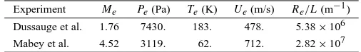
of the hypersonic range. In this flow, first effects of compressible turbulence may be expected. The experiment was carried out by Mabey et al. (Fernholz and Finley [9]). This last experiment has been chosen recently as a test-case for the ETMA Workshop (Hirsch and Shang [40]) and several computations with different turbulence models are available on this configuration. It is fully documented as test-case ID No. 7402 in AGARDograph No. 223 (Fernholz and Finley [9]). The characteristics of each flow are recalled in table I.
Table I. Characteristics of the boundary layers.
Experiment Me Pe(Pa) Te(K) Ue(m/s) Re/L(m−1)
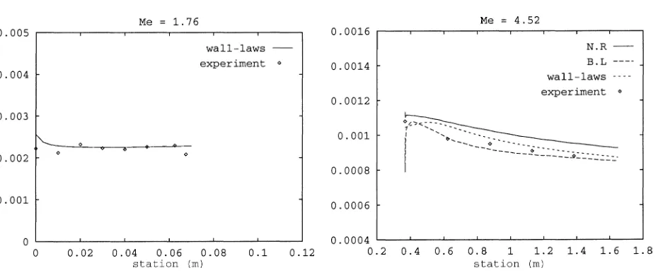
Figure 7. Friction coefficient for the wall-function approach; left:Me=1.76, right:Me=4.52.
4.2. Performances of thek–εmodel with wall-function approach
4.2.1. Standardk–εmodel
We first present the results obtained with the standardk–ε model using wall functions before analyzing the results obtained with the modified models.
Figure 7 presents the variation of the skin friction coefficient versus the horizontal coordinate. It can be
seen that results are in very reasonable agreement with experimental data. Figure 7 also presents results obtained on the Mabey Mach 4.52 experiment during the ETMA workshop (Hirsch and Shang [40]) by different investigators using turbulence models which have not been tested in the present work. B-L stands for a Baldwin–Lomax model used by Hirsch and Shang [40] and R-N represents the results obtained by Hughes et al. [41] using the one-equation model of Reynolds–Norris. The comparisons between computations and measurements show that the agreement of the present work (k–εmodel with wall functions) with experimental data is as good as (or even better than) the results obtained with various models tested during this workshop.
Figure 8 displays the velocity profiles plotted in wall coordinates for the two flows under study. Again in
the two cases, the agreement with the experiments is quite good and the k–ε model, associated with wall functions, gives a correct law of the wall. The agreement is very good for the case with a moderate value of the Mach numberMe=1.76, at a rather low-Reynolds numberRδ2=3000. First hints of a discrepancy appear
in the case of Mabey forMe=4.52. The overall agreement can be considered as satisfactory. However, more
careful analysis of the results in figure 9 indicates an unexpected behavior of the computed law of the wall: the extent of the logarithmic zone in terms ofy+ is shorter for Mabey’s case, although the Reynolds number is larger(Rδ2≃7000). This result suggests that at the limit of the hypersonic regime, the present model starts
having difficulties in reproducing a correct matching between viscous and non-viscous zones. The analysis proposed by Huang et al. [4] points out that in the presence of significant density gradients, thek–ε model is not consistent with the logarithmic law. Indeed, a closer examination of the results shows that the standard
Figure 8. Van Driest transformed velocity in wall coordinates; left:Me=1.76, right:Me=4.52 (wall-function approach).
Figure 9. Van Driest transformed velocity in wall coordinates.
grows slightly past the inlet section. However, we note that this effect is rather small. According to Fernholz and Finley [9] the accuracy of measurement for Cf is of the order of 7% for Mabey’s experiment and, in
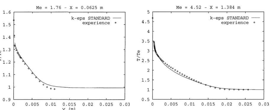
the last section, the numerical results are within the limit of the experimental accuracy. Figure 10 displays a comparison of the experimental data with the results of the standard k–ε model on the temperature fields at the last measurement station for the two different Mach numbers. It can be noticed that the overall agreement with the experimental data is good and of similar quality for the two test cases. Therefore with respect to the temperature field, the presence of compressible effects in the Mach 4.52 experiment does not seem to alter the performance of the model.
4.2.2. Compressibility modelling
Figure 10. Temperature in the last measurement station; left:Me=1.76, right:Me=4.52.
(Viegas and Rubesin [42], Guézengar and Guillard [32]) with large success (it seems however that the accuracy of these models decreases when an important density ratio is present between the two streams, see Guézengar et al. [43]. Some applications of compressibility corrections have also been made for boundary layers (Huang et al. [4], Mohammadi and Pironneau [6], Aupoix et al. [5]) and we tried them on computations using thek–ε
model associated with wall functions.
Compressibility corrections are based on the turbulent Mach number, so it is interesting to know what is the range ofMt involved in the two test-cases which we have considered. For theMe=1.76 experiment, it appears
that the turbulent Mach number reaches a maximum value of 0.197. This value is too low for Wilcox’s model to act. The action of other models is very weak (they modify the value of the dissipation by less than 2%) and therefore no significant action of the compressible corrections can be noticed on this flow.
In the case of the Mabey experiment, the turbulent Mach number reaches a maximum value of 0.276. Although this value is low compared to the values reached in mixing layers, compressibility models can have an influence on the results for this flow. This is indeed the case, as can be seen in figure 11 which shows the velocity profiles in wall coordinates obtained by the different models. However, such corrections tend to overestimate the slope of the velocity profile compared with the classical logarithmic law. In fact, compressibility models increase the dissipation term in the k-equation and thus reduce the turbulent kinetic energy level. In the logarithmic region, the decrease ofkimplies an increase of the slope of the velocity profile. Therefore, this kind of model is not suitable for boundary layer computations. This is the conclusion which was already reached by Huang et al. [4]. It is possible to reinterpret this result in the light of the works of Ristorcelli [28] and of Fauchet et al. [30]. In the logarithmic zone of a boundary layer, it will be assumed that
P∼εt, and following Ristorcelli’s analysis the pressure-divergence term may be neglected. Then, we can focus
on the compressible dissipation. The work by Fauchet et al. [30] gives some indication of the level of this term. Their simulations of compressible isotropic turbulence suggests that
εc=εA
lnRl Rl
Mt4,
whereRl=ul/ν,Mt =u/awithu=
√
Figure 11.Me=4.52: Compressibility corrections—log-layer velocity profile comparisons atx=1.384 m (wall-function approach). results as follows; it is clear that in a shear flow, the value of constant A has probably to be revised. However, we assume that putting A=1 gives the right order of magnitude forεc. The scale l was estimated from the
relationε=k3/2/ lin the equilibrium zone whereP∼ε. In this case,
l=Cµ3/4κy.
Now, we have to evaluate the factor lnRl/Rl. It turns out that this quantity remains smaller than 0.37 and is
about 0.2 in the zone of interest for our computations. Finally, the resulting estimation forεc is
εc∼0.3εMt4.
In the present computations, the maximum value for ofMt is 0.276 in Mabey’s experiments. This would give
a maximum value of compressible dissipationεc∼1.2×10⁻³ε. Therefore, according to this theory, the level
of compressible dissipation is three orders of magnitude below the solenoidal one, and it can be neglected. This is consistent with the simulations of Huang et al. [23]. This is also in qualitative agreement with the classical description of non-hypersonic boundary layers. This suggests that the recent models forεcgive a level
of dissipation acceptable for equilibrium boundary layers up toM =5, and in that respect, seem to have a sounder behaviour than the former models inM2
t.
4.2.3. Density gradient correction
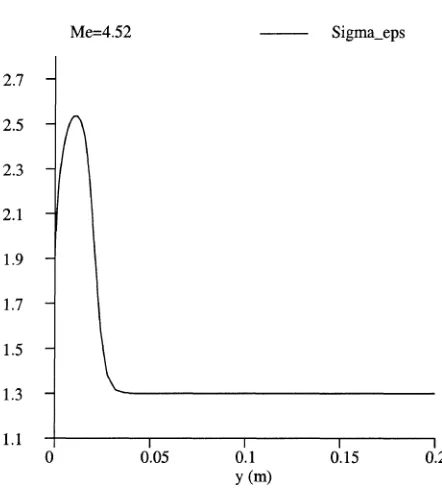
Figure 12.Me=4.52:σεprofile across the layer atx=1.384 m.
For the Dussauge Mach 1.76 experiment, the density gradients across the layer are moderate and the results obtained with the standardk–ε model with the constant σε=1.3 are in good agreement with the logarithmic
law. It has been checked that the introduction of the variable σε model (14) does not modify this behavior.
Results obtained with the modified model are almost the same as the ones obtained with the standard model. Moreover, from a numerical point of view, the introduction of this model does not modify the behavior of the numerical algorithm.
The situation of the Mabey et al. Mach 4.52 experiment is very different. In this experiment, the density ratio between the free stream density and the density at the wall is almost 5 and therefore we expect the density correction to have a significant influence on the value of σε. In figure 12 we see that indeed the
coefficient σε experiences a large variation across the layer from its free stream value of 1.3 to a maximum
of 2.5 in the boundary layer. In figure 13 we can see that this variation has a significant impact on the results. Clearly the effect of the density gradient correction of theσε coefficient is to allow a better agreement with the
compressible log-law. Actually, with the standardk–ε model, the velocity slope departs rapidly from the curve log(y+)/0.4+5.1 while the modified model follows this curve betweeny+∼30 andy+∼400. The density correction produces therefore the expected trend. However, we also see that it tends to destroy the wake-law. In fact, it seems that this correction extends too far outside the logarithmic zone and forces the turbulent balance between production and dissipation also in the external zone.
4.3. Near-wall modelling influence
4.3.1. Low-Reynolds number models
Figure 13.Me=4.52: Density gradient corrections—log-layer velocity profile comparisons atx=1.384 m (wall-function approach).
Figure 14.Me=4.52: Friction coefficient for two-equation low-Reynolds number models.
that this results from the adjustment between the inlet boundary conditions and the internal dynamics of the modelled equations. However, very soon after the inlet boundary, models give a friction coefficient with a correct behavior and the numerical results are in reasonable agreement with experimental data. The Speziale– Abid–Anderson model gives a prediction closer to the experimental points, probably due to the particular response of the model to inlet conditions. Further inspection of these results suggests that, although the absolute level of the skin friction is too low, the variations ofCf versus x found with Nagano–Tagawa’s model are in
Figure 15.Me=4.52: Comparison of horizontal momentum for the-two equation low-Reynolds number models atx=1.384 m.
Figure 16. Normalized turbulent kinetic energy versusy+;Me=4.52 (Lam–Bremhorst model).
Although no experimental data is available on the turbulent kinetic energy, it can be interesting to consider the prediction of the low-Reynolds models for this quantity and to check if one can notice an influence of the compressibility on the behavior of the turbulent kinetic energy. Figure 16 displays the normalized turbulent kinetic energy defined as k+=ρk/(ρpu2τ) versus the normalized wall distance y+ in the last measurement
Figure 17. Normalized dissipation versusy+;Me=4.52 (Lam–Bremhorst model).
Figure 17 displays the behavior of the normalized dissipation rate defined as ε+ =(ρ3/2ενw)/(ρw3/2u 4 τ)
versus the normalized distance to the wall. Once again, we note that the results do not differ from the known incompressible ones. The normalized dissipation reaches a maximum∼0.18 fory+∼11.5. These values are compatible for instance with the data of Laufer [44] that give a maximum of∼0.2 fory+∼9. The main point to be noticed is that for this high velocity boundary layer, the low-Reynolds models continue to behave as in the incompressible case. Finally, note that theε+curve exhibits a slight oscillation near the wall. It is believed that this oscillation is a numerical artifact due to the change in the definition of the parameters Rt, Ry in the
near wall treatment (see Eq. (16)).
From a numerical point of view, it is worth noting that these low-Reynolds number models require a very fine mesh as compared to the wall law models to yield accurate results. In the present case, a mesh of 113×81 with an aspect ratio of 5000 near the solid wall was necessary to give results in fair agreement with the data. The CPU time necessary to get a converged solution is of the order of 30 min on a Dec Alpha 600/266 MHz workstation. This has to be compared with the 5 min needed by the k–ε model with wall functions.
4.3.2. Two-layer model
Figure 18.Me=4.52: Friction coefficient for the two-layer model on a 57×41 and a 113×81 mesh.
Figure 19.Me=4.52: Van Driest transformed velocity profile atx=1.384 m (two-layer model).
5. Conclusions
We have applied several variations of the baseline k–ε model to the computations of supersonic boundary layers on flat adiabatic plate. Apart from the fact that on the average the models (including the baseline k–ε
model using wall functions) show a good agreement with the experimental data, the main conclusions of this study are the following:
– From a numerical standpoint, the two-equation low-Reynolds number models are fragile and experience serious convergence difficulties when applied in their basic form. However, when they are used in combination with the boundary condition (9) and the modified parameter Rt described in (16), the
robustness of such models is greatly increased and their CPU cost is of the same order as the CPU cost of the two-layer model on the same mesh. However, such models seem to be very sensitive to the inlet boundary conditions. It is likely that this sensitivity comes from the initial specification of the dissipation rate.
– The two-layer model is not subject to the same numerical difficulties as the low-Reynolds number models. Moreover, it exhibits a reduced sensibility to the specification of the boundary conditions. It seems therefore that this kind of model offers good potentialities for the computation of compressible flows.
– In agreement with Huang et al. [4], we found that the compressibility models, in their present form, are not efficient in supersonic boundary layer computations. The use of a two layer model, conveniently adapted to variable density flows, leads to a better prediction ofCf than the wall-function approach and the
low-Reynolds number models investigated. For the shape of the velocity profiles, the overall agreement is very good at moderate supersonic Mach numbers, and is fair at the limit of the hypersonic range. In particular at Mach number 4.52 for adiabatic wall conditions, the slope of the logarithmic zone is not correctly predicted, and the use of corrections for density gradients would probably required. Finally, the density gradient correction that we have designed to cure this possible problem is effective in enforcing the turbulence balance. In our experiments, it appears actually to be too effective as it enforces the turbulent balance also in the wake region; a simple cure for this problem can be to limit the extend of the correction to the logarithmic region.
Appendix
The model of Lam–Bremhorst
The damping functions are defined by
The model of Nagano–Tagawa
The damping functions are defined by
The damping functions are defined by
The first author (D. Guézengar) was supported by CEA/CESTA under contract No. 195 E03100 41606. This support is gratefully acknowledged. The authors would like to thank A. Dervieux, B. Mohammadi of INRIA and M. Ravachol of Dassault Aviation for the interesting discussions and advice that they provided in the course of this study. The inlet boundary conditions for the turbulent variables used for the Mabey et al. experiment were by courtesy of I. Yudiana and M. Buffat of Ecole Centrale de Lyon. The inlet boundary conditions for the Dussauge et al. experiment were produced by a program due to R. Arina of Politecnico di Torino. We thank them warmly for their help in these matters.
References
[1] Van Driest E.R., Turbulent boundary layer in compressible fluids, J. Aeronaut. Sci. 18 (1951) 145–160. [2] Bradshaw P., Compressible turbulent shear layer, Annu. Rev. Fluid Mech. 9 (1977) 33–54.
[3] Fernholz H.H., Finley P.J., A critical commentary on mean flow data for two-dimensional compressible turbulent boundary layers, AGARDo-graph 253 (1980).
[4] Huang P.G., Bradshaw P., Coakley T.J., Turbulence model for compressible boundary layers, AIAA J. 32 (1994) 735–740.
[5] Aupoix B., Desmet E., Viala S., Hypersonic turbulent boundary layer modelling, in: Symposium on Transitional and Compressible Turbulent Flows, Washington, DC, ASME Fluids Engineering Conference, 1993.
[6] Mohammadi B., Pironneau O., Compressibility corrections and two-layerk–εmodels for hypersonic turbulent flows on unstructured grid, Comp. Fluid Dynam. 4 (1995) 285–306.
[8] Fernholz H.H., Finley P.J., A survey of measurements and measuring techniques in rapidly distorted compressible turbulent boundary layers, AGARDograph 315 (1989).
[9] Fernholz H.H., Finley P.J., A critical compilation of compressible turbulent boundary layer data, AGARDograph 223 (1977).
[10] Lam C.G.K., Bremhorst K., A modified form of thek–εmodel for predicting wall turbulence, J. Fluid Eng-T ASME 103 (1981) 456–460. [11] Nagano Y., Tagawa M., An improvedk–εmodel for boundary layer flows, J. Fluid Eng-T ASME 112 (1990) 33–39.
[12] Speziale C.G., Abid R., Anderson E.C., A critical evaluation of two-equations models for near wall turbulence, ICASE Report 90-46, 1990. [13] Smith A.J., Dussauge J.-P., Turbulent Shear Layers in Supersonic Flow, AIP, Noodburry, NY, 1996.
[14] Aupoix B., Viala S., Compressible turbulent boundary layer modelling, in: Symposium on Transitional and Compressible Turbulent Flows, The Westin Resort, Hilton Head Island, SC, 1995.
[15] Chapman D.R., Kuehn G.D., Navier–Stokes computations of viscous sublayer flow and the limiting behaviour of turbulence near a wall, in: AIAA 7th Computational Fluid Dynamics Conference, Cincinatti, OH, AIAA, New York, 1985.
[16] Wolfshtein M., The velocity and temperature distribution in one-dimensional flow with turbulence augmentation and pressure gradient, Int. J. Heat Mass Trans. 12 (1969) 301–318.
[17] Viala S., Effets de la compressibilité et d’un gradient de pression négatif sur la couche limite turbulente, Thesis, ENSAE, Toulouse, 1996. [18] Sarkar S., Erlebacher G., Hussaini M.Y., Kreiss H.O., The analysis and modelling of dilatational terms in compressible turbulence, ICASE
Report 89-1789, 1989.
[19] Zeman O., Dilatation dissipation: the concept and application in modeling compressible mixing layers, Phys. Fluids A-Fluid 2 (1990) 178–188. [20] Sarkar S., Erlebacher G., Hussaini M.Y., Compressible homogeneous shear: simulation and modeling, ICASE Report 92-6, 1992.
[21] Wilcox D.C., 1992, Dilatation–dissipation corrections for advanced turbulence models, AIAA J. 30 (1992) 2639–2646. [22] Sarkar S., The stabilizing effect of compressibility in turbulent shear flow, J. Fluid Mech. 282 (1995) 163–186. [23] Huang P.G., Coleman G., Bradshaw P., Compressible turbulent channel flows, J. Fluid Mech. 305 (1995) 185–218.
[24] Freund J.B., Moin P., Lele S.K., Compressibility effects in a turbulent annular mixing layer, Report No. TF-72, Flow Physics and Computation Division, Department of Mechanical Engineering, Stanford University, Stanford, CA, 1997.
[25] Durbin P.A., Zeman O., Rapid distortion theory for homogeneous compressed turbulence with application to modelling, J. Fluid Mech. 242 (1992) 349–370.
[26] Jacquin L., Cambon C., Blin E., Turbulence amplification by a shock wave and rapid distortion theory, Phys. Fluids A-Fluid 2 (1993) 949–954. [27] Simone A., Coleman G., Cambon C., The effect of compressibility on turbulent shear flow: a rapid-distortion-theory and
direct-numerical-simulation, J. Fluid Mech. 330 (1997) 307–338.
[28] Ristorcelli J.R., A pseudo-sound constitutive relationship for the dilatational covariances in compressible turbulence, J. Fluid Mech. 347 (1997) 37–70.
[29] Ristorcelli J.R., Blaisdell G., Consistent initial conditions for the DNS of compressible turbulence, Phys. Fluids 9 (1997) 4.
[30] Fauchet G., Shao L., Wunenburger R., Bertoglio J.P., An improved two-point closure for weakly compressible turbulence and comparisons with LES, in: 11th Symposium on Turbulent Shear Flows, Grenoble, September 8–11, 1997.
[31] Fauchet G., Modélisation de la turbulence isotrope compressible et validation à l’aide de simulations numériques, Thèse de Doctorat, Univ. Claude Bernard, Lyon, 1998.
[32] Guézengar D., Guillard H., Compressibility models applied to supersonic mixing layers, in: Dervieux A. et al. (Eds), Proc. ETMA Workshop, Notes on Numerical Fluid Mechanics, Vieweg, Braunschweig/Wiesbaden, 1998.
[33] Guézengar D., Modélisation et simulation numérique de la turbulence compressible dans les écoulements cissaillés supersoniques, Thesis, University of the Méditerranée, Marseille, 1997.
[34] Larrouturou B., How to preserve the mass fraction positivity when computing compressible multi-component flows, J. Comput. Phys. 1 (1991) 59–84.
[35] Fezoui L., Lanteri S., Larrouturou B., Olivier C., Résolution numérique des équations d’Euler en plusieurs dimensions, INRIA Report 1033, 1989.
[36] Dervieux A., Steady Euler simulations using unstructured meshes, in: Geymonat G. (Ed.), Partial Differential Equations of Hyperbolic Type and Applications, Von Karman Institute Lecture Series 85-04, World Scientific, Singapore, 1985, pp. 34–105.
[37] Olivier C., Larrouturou B., On the numerical approximation of thek–εmodel for two dimensional compressible flow, INRIA Report 1526, 1991.
[38] Guillard H., Mixed Element Volume Methods in CFD, Von Karman Institute Lecture Series 95-02, 1995. [39] Wilcox D.C., Turbulence Modeling for CFD, Griffin Printing, Glendale, CA, 1993.
[40] Hirsch C., Shang E., Synthesis on test-case TC3 of ETMA workshop, in: Dervieux A. et al. (Eds), Proc. ETMA Workshop, Notes on Numerical Fluid Mechanics, Vieweg, Braunschweig/Wiesbaden, 1998.
[41] Hughes T.J.R., Jansen K., Hauke G., Application of the finite element method to the Reynolds-averaged Navier–Stokes equations, in: Der-vieux A. et al. (Eds), Proc. ETMA Workshop, Notes on Numerical Fluid Mechanics, Vieweg, Braunschweig/Wiesbaden, 1998.
[42] Viegas J.R., Rubesin M.W., A comparative study of several compressibility corrections to turbulence models applied to high-speed shear layers, AIAA Paper 91-1783, 1991.
[43] Guézengar D., Guillard H., Dussauge J.-P., Compressibility and density gradients in the modelling of the dissipation equation: application to turbulent shear flows, in: Jourdan G., Houas L. (Eds), Proc. 6th International Workshop on the Physics of Compressible Turbulent Mixing, CARACTERE, Marseille, 1998, pp. 185–190.